Modelling financial markets using methods from network theory.

(1)

Modelling Financial Markets using

Methods from Network Theory

Thesis submitted in accordance

with the requirements of the

University of Liverpool for the

degree of Doctor in Philosophy

by Jenna Louisa Birch

(2)

Abstract

This thesis discusses how properties of complex network theory can be used to study financial time series, in particular time series for stocks on the DAX 30.

First, we make a comparison between three correlation-based networks: minimum spanning trees; assets graphs and planar maximally filtered graphs. A series of each of these network types is created for the same dataset of time series’ of DAX 30 stocks and we consider what information each network can provide about the rela-tionship between the stock prices from the underlying time series. We also analyse two specific time periods in further detail – a period of crisis and a period of recovery for the German economy.

Next, we look at the structure and representations of planar maximally filtered graphs and in particular we consider the vertices that form the 3-cliques and 4-cliques [Tumminello et al. (2005)] state ‘...normalizing quantities are ns − 3 for 4-cliques and 3ns−8 for 3-cliques. Although we lack a formal proof, our investiga-tions suggest that these numbers are the maximal number of 4-cliques and 3-cliques,

respectively, that can be observed in a PMFG of ns elements.’ Within this thesis we provide a proof for these quantities and a different construction algorithm.

(3)

Publications

The Maximum Number of 3- and 4-Cliques Within a Planar Maximally Filtered Graph. J. Birch, A.A. Pantelous and K. Zuev. (2015).

Physica A: Statistical Mechanics and its Applications. Vol. 417 (Iss. C) 221-229.

Analysis of Correlation Based Networks Representing DAX 30 Stock Price Returns. J. Birch, A.A. Pantelous and K. Soram¨aki. (2015).

Computational Economics. DOI 10.1007/s10614-015-9481-z.

Conference Presentations

• Forecasting Financial Markets 2013, Hannover, Germany (29/05/13 - 31/05/13),

• 60th ISI World Statistics Congress 2015, Rio de Janeiro, Brazil (26/07/15 -31/07/15).

Conferences and Workshops Attended

• SCOR Conference, University of Nottingham, Nottingham (20/04/12 - 22/04/12),

• Financial Network Workshop: Hosted by FNA, Pompeu Fabra University, Barcelona (03/05/12 - 05/05/12),

• LMS EPSRC: Common Themes in Financial & Actuarial Mathematics, Man-agement School, University of Liverpool, Liverpool (15/04/13 - 19/04/13),

(4)

• NetSci 2014 School and Conference, University of California, Berkeley (02/06/14 - 06/06/14),

(5)

Acknowledgements

I would like to express my appreciation and thanks to my supervisor Dr. Pantelous for your advice and guidance, and for providing me with so many opportunities over these past four years. Also to my second supervisor Dr. Zuev, thank you for your contributions over the past year, and for your time, patience and dedication to my research. To those at FNA, particularly Kimmo Soram¨aki, thank you for the intern-ship opportunity. Your constant support over the years has been much appreciated and I hope to continue working with you in the future.

I would not have been able to complete my thesis without the help of people within the Department of Mathematics and particularly the members of IFAM. This re-search would not have been possible without the funding through the GTA scheme. I would like to specifically mention Dr. Constantinescu, your advice and believe in me over the years have helped me during the times I’ve needed support the most and Jia Shao (Sara), I appreciate your help with proof-reading and problem solving but most of all I appreciate what a good friend you have been to me.

There are friends from each stage at university, including some of the lovely girls at LULHC and also from outside of university that have kept me sane at times with good advice, laughter and tea breaks I feel a list would certainly miss people out so I would like to thank you collectively and I know that this work would not have been completed without you all.

(6)

List of Figures

1 The time series shows the quarter-on-quarter volume growth of GDP and expenditure components for Germany (shown in blue) and the euro area (shown in red). . . 14 2 The first six vertices (labelled using the stock’s ticker symbol) and

five edges of the MST extracted from data showing the correlation between the daily returns of the closing prices for the 30 members of the DAX 30 from 5th February 2001 - 7th March 2001. . . 25 3 The complete MST extracted from data showing the correlation

be-tween the daily returns of the closing prices for the 30 members of the DAX 30 from 5th February 2001 - 7th March 2001. The vertices are labelled using the stock’s ticker symbol and have been coloured to highlight the clusters so they can be compared to the AG for the same time period (see Figure 5). . . 25 4 The hierarchical tree extracted from Table 2. The vertices are shown

along the x-axis labelled by their ticker symbol. The ultrametric dis-tance is shown on the y-axis. . . 27 5 The complete AG extracted from data showing the correlation

(9)

6 Times series of the daily closing price, adjusted for dividends and splits between 1st September 2007 and 1st September 2009. The red markers indicate the individual days. . . 41 7 A quadrilateral ABCD is formed by the two adjoining triangles ABC

and ACD which share a common edge (A,C). If we perform a diagonal flip the edge (A,C) is replaced by the edge (B,D). . . 49 8 This PMFG with 6 vertices highlights the two possible 3-cliques.

Ver-tices A,C,D form a 3-clique and they outline a triangle on the surface. Vertices A,B,E also form a 3-clique however they do not outline a surface triangle but rather the edges enclose 3 surface triangles which share common edges. A,B,E forms a separating 3-cycle. . . 50 9 PMFGs with n = 8 and deg[vA, vB, vC, ..., vH]=[7, 5, 5, 5, 4, 4, 3, 3].

These graphs are isomorphic and have C3 = 16 and C4 = 5. . . 53

10 Both graphs havedeg[vA, vB, vC, ..., vH]=[6, 6, 5, 5, 4, 4, 3, 3] however they are not isomorphic and so are not planar representations of a single graph. Furthermore, they have different numbers of C3 and C4

with the graph shown in Panel (a) having C3 = 16, C4 = 5 and the

graph shown in Panel (b) having C3 = 14, C4 = 2. . . 53

11 A maximal graph withnvertices in the standard spherical triangulation. 54 12 Panel (a) - The first Eberhard operation, ϕ1, Panel (b) - The second

Eberhard operation, ϕ2, Panel (c) - The third Eberhard operation,

ϕ3. (Presented in [Eberhard (1891)]). . . 56

13 Panel (a) Standard spherical triangulation form, withC3 = 10,C4 = 3

and Panel (b) the alternative form, with C3 = 8, C4 = 0. . . 57

(10)

15 The transformation of P5 to P6 using Eberhard operation ϕ1. . . 58

18 An example of a VG constructed from the time series: 0.698, 0.269, 0.597, 0.178, 0.422, 0.881, 0.030. A bar chart is created, the visible data are connected and the corresponding VG is shown underneath. . 66

19 An example of a HVG constructed from the time series: 0.698, 0.269, 0.597, 0.178, 0.422, 0.881, 0.030. A bar chart is created, the visible data are connected using horizontal lines and the corresponding HVG is shown underneath. . . 67

20 Graph showing the degree distribution for each stock from the full set of n=11011 days along with the theoretical probability given by P(k) = (1 3)( 2 3) k−2 _{as shown by [Luque}_{et al.} _{(2009)]. . . .} ₇₄

21 The minimum spanning tree for 7th October - 6th November 2008. . 95

22 The minimum spanning tree for 21st October - 20th November 2008. 96 23 The minimum spanning tree for 4th November - 4th December 2008. 96 24 The minimum spanning tree for 18th November - 18th December 2008. 97 25 The minimum spanning tree for 2nd December - 31st December 2008. 97 26 The asset graph for 7th October - 6th November 2008. . . 101

27 The asset graph for 21st October - 20th November 2008. . . 101

28 The asset graph for 4th November - 4th December 2008. . . 102

29 The asset graph for 18th November - 18th December 2008. . . 103

30 The asset graph for 2nd December - 31st December 2008. . . 103

(11)

32 The planar maximally filtered graph for 21st October - 20th November

2008. . . 104

33 The planar maximally filtered graph for 4th November - 4th December 2008. . . 105

34 The planar maximally filtered graph for 18th November - 18th De-cember 2008. . . 105

35 The planar maximally filtered graph for 2nd December - 31st Decem-ber 2008. . . 106

36 The minimum spanning tree for 7th May - 8th June 2010. . . 107

37 The minimum spanning tree for 21st May - 22nd June 2010. . . 108

38 The minimum spanning tree for 4th June - 6th July 2010. . . 108

39 The minimum spanning tree for 18th June - 20th July 2010. . . 109

40 The minimum spanning tree for 2nd July - 3rd August 2010. . . 109

41 The asset graph for 7th May - 8th June 2010. . . 113

42 The asset graph for 21st May - 22nd June 2010. . . 113

43 The asset graph for 4th June - 6th July 2010. . . 114

44 The asset graph for 18th June - 20th July 2010. . . 115

45 The asset graph for 2nd July - 3rd August 2010. . . 115

46 The planar maximally filtered graph for 7th May - 8th June 2010. . . 116

47 The planar maximally filtered graph for 21st May - 22nd June 2010. . 116

48 The planar maximally filtered graph for 4th June - 6th July 2010. . . 117

(12)

List of Tables

1 The table shows Germany’s exports and imports as a percentage of Gross Domestic Product (GDP). The data is taken from ‘German Foreign Trade in 2014’, a report by Germany’s Federal Ministry for Economic Affairs and Energy. . . 17 2 The first nine ordered distances for the MST construction from 5th

February 2001 - 7th March 2001. . . 24 3 The table shows the ultrametric distances between the first six

ver-tices added to the MST extracted from data showing the correlation between the daily returns of the closing prices for the 30 members of the DAX 30 from 5th February 2001 - 7th March 2001, with the stocks labelled using their ticker symbols. . . 28 4 The table shows the number of stocks for each time period, within

the overall crisis period, the number of 4-cliques that formed, the maximum number of 4-cliques possible for that time period and how many of the cliques were made up of stocks from 4 different economic sectors, 3 different sectors, 2 different sectors or all from the same economic sector. . . 39 5 The table shows the number of stocks for each time period, within

(13)

7 The mean degree of the HVG for the 18 stocks (labelled using their ticker symbols for a period of crisis (2008 - 2009) and a periods of recovery (2010 - 2011)). . . 72 8 The clustering coefficient of the HVG for the 18 stocks (labelled using

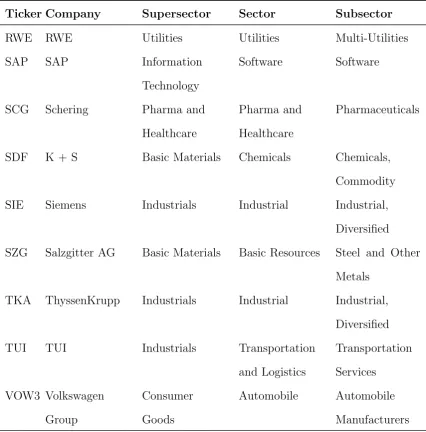
their ticker symbols for a period of crisis (2008 - 2009) and a periods of recovery (2010 - 2011)). . . 73 9 List of all stock symbols and the supersector, sector and subsector

that the company belongs to. The details of the various sectors can be found in Guide to the Equity Indices of Deutsche B¨orse. Version 6.6, November 2008 (http://www.Deutscheboerse.com). . . 88 10 The edges that form the asset graph for 7th October - 6th November

2008. . . 98 11 The edges that form the asset graph for 21st October - 20th November

2008. . . 99 12 The edges that form the asset graph for 4th November - 4th December

2008. . . 99 13 The edges that form the asset graph for 18th November - 18th

De-cember 2008. . . 100 14 The edges that form the asset graph for 2nd December - 31st December

(14)

(15)

1 Introduction

(16)

(17)

between two stocks if the cross correlation was larger than a particular threshold value. This method was also used by [Qiu et al. (2010)] to study the dynamical behaviour of American and Chinese stock markets.

(18)

graph into two disconnected parts. For the PMFG we consider the vertices that form the 3- and 4-cliques (as the maximum number of elements that can form a clique is 4). [Tumminelloet al. (2005)] state‘...normalizing quantities arens−3for 4-cliques and3ns−8 for 3-cliques. Although we lack a formal proof, our investigations suggest that these numbers are the maximal number of 4-cliques and 3-cliques, respectively,

that can be observed in a PMFG of ns elements.’ One way that we use the cliques to analyse networks is to consider the ratio between the number of cliques that have formed to the maximum number of cliques that could form. For this, [Tumminello et al. (2005)] used the normalizing quantities that have been mentioned above, an approach that has also been used by [Eryigit & Eryigit (2009)], [Asteet al. (2005a)] and [Tumminelloet al. (2007)] and used when defining the connection strength of a sector by [Coronnello et al. (2005)]. Within Chapter 4 of this thesis we provide a proof for these quantities and a different construction algorithm.

(19)

the relationship between the stock prices from the underlying time series. We also analyse two specific time periods in further detail – a period of crisis and a period of recovery for the German economy. Our aim is to test whether or not there is a difference between the networks created from the two datasets and, if so, what information we can extract about the stocks during these time periods.

(20)

such as degree distribution, average path length and clustering coefficient, and as stated above, these can reflect certain properties of the time series. For example, if we create a visibility graph for a periodic time series then the network will inherit the regularity of the time series and as such will be a regular network. By similar reasoning the algorithm also creates an exponential random network from a random times series and a scale-free network from a fractal time series [Lacasaet al. (2008)].

The literature in this area mainly covers theoretical results. For example [Luqueet al. (2009)] showed that a Horizontal Visibility Graph (HVG) generated from a bi-infinite random time series will have a degree distribution ofP(k) = (1₃)(2₃)k−2_. _This

(21)

algo-rithms have been applied to time series from various fields such as physics datasets and financial time series. Modelling energy dissipation rates in turbulence using VGs, [Liu et al. (2009)] looked at the statistical properties and found the degree distribution to be power-law, P(k)∼k−α where α=−3. [Yu et al. (2012)] applied the horizontal visibility algorithm to daily time series of the solar x-ray brightness from 1986 - 2007 and found that multifractality exists in both the daily time series and the corresponding HVGs. In [Yang et al. (2009)] VGs were constructed from six exchange rate series (US dollars to Australian dollars, Canadian dollars, euro, GB pound, Japanese Yen and NZ dollar.) The authors considered the original time series, as well as shuffled and detrended data, and found that the series converted to a scale-free and hierarchically structured network, also the original and detrended time series were multifractal. The hierarchies for the Yen and euro came across weaker compared to the others. In Chapter 5 of this thesis we present the formal construction algorithm for VG and HVGs. We discuss the properties of the graphs created from the time series and proven results from the literature. Finally, we con-sider whether the family of visibility algorithms is an appropriate method to apply to financial time series.

(22)

(23)

2 Financial Network Theory

In this chapter we introduce some of the key terminology from Network Theory that is used throughout this thesis. We also discuss the euro area, in particular details of the German economy for 2001 – 2014 as this time period covers the dataset used in later chapters. Our discussions include the introduction of the euro, Germany’s imports and exports and the German stock market, the DAX 30.

2.1 Preliminaries

Anetwork, also referred to in literature as agraph, is a set ofvertices (or nodes) con-nected by edges. Denote the graph G(V, E) whereV is the set of vertices belonging toGandE is the set of edges belonging toG. Denote the number of vertices|V|=n

and the number of edges|E|=m. Aloop is an edge whose end vertices coincide and amultiple edge is formed when two or more edges join the same vertices. If a network does not contain any loops or multiple edges then it is called a simple network. A subgraph H, of a graphG(V, E), is a graph whose vertices are a subset of the vertex setV and whose edges are a subset of the edge setE. A subset of vertices C∈V is called aclique if the subgraphG(C) is a complete graph (a simple graph with every pair of distinct vertices connected by a distinct edge) and is denotedCjwhere|C|=j.

(24)

closed loops. A network can bedirected or undirected depending on whether or not the edges show the direction of the flow between the vertices. If the flow between vertices can only be one way then the edge is called a directed edge (or alternatively anarc) and thus it follows that a network consisting of directed edges is simply called a directed network (or a digraph). An undirected edge has a two-way flow between vertices. Note that an undirected network can be transformed into a directed one by representing the undirected edges between the vertices as two directed edges. As well as the direction of the edges we also consider the values assigned to the edges. A weighted network is one in which the edges between the vertices have weights as-signed to them. Depending on the subject of the network these weights can have different meanings. For example, it could show a cost of ‘using’ an edge or the total flow allowed to travel through the edge. In financial models it could be the values or volume traded. If no value is assigned then there is assumed to be unlimited flow throughout the network and the network itself is described as anunweighted network. The edges can be scaled to reflect these weights either by edge length or thickness.

(25)

(for example degree and mean degree).

The number of edges adjacent to a vertex is known as thedegree of the vertex. For a vertex, v, we use the notation deg(v) to show the degree, or alternatively ki. In any network, the sum of the degrees of all the vertices is equal to twice the number of all edges, i.e. for a networkG(V, E), with n verticesvi (wherei= 1, ..., n):

n

X

i=1

deg(vi) = 2|E|. (1)

The mean degree for a network is calculated as:

1

n

X

i=1

ki = 2|E|

|V| . (2)

A vertex can be classed as either an odd or even vertex depending on whether the degree of the vertex is odd or even. In a directed network the number of edges coming into a vertex is called theindegree and the number of edges leaving a vertex is called theoutdegree. The following equation holds for all directed networks:

X

v∈V

indeg(v) =X v∈V

outdeg(v) =|E|. (3)

In a directed network a vertex with indegree = 0 is called the source (and can be seen as the origin) whilst a vertex with outdegree = 0 is called thesink. If a vertex,

(26)

When considering large scale networks an important property to consider is the degree distribution. Let P(k) be the percentage of vertices with degree k in the network. Thedegree distribution is the distribution ofP(k) over all k, i.e. the prob-ability that a vertex has degreek. When constructing a random network, vertices are added at random meaning that there tends to be an average degree. This results in the degree of most of the vertices within the network distributed around this average with few vertices having a much higher or lower degree. However, real life networks have been shown to have a much more skewed distribution with most vertices hav-ing only a few edges and a (proportionally) small number of vertices behav-ing highly connected with a large degree value. This leads to a power-law distribution where

P(k)∼k−γ. A network that demonstrates a power-law degree distribution is known as a scale-free network.

(27)

form an open triplet and three vertices joined by three edges form a closed triplet).

C= Number of closed triplets_{Number of total triplets} , where C = 1 implies perfect transitivity.

Further details on network theory can be found in [Albert & Barab´asi (2002)] and [Newman (2010)].

2.2 German Economy

In Chapter 3 we analyse the DAX 30 blue chip stocks for the time period 2001 - 2014 (see Appendix A for a list of all stock symbols and the sectors to which they belong and Section 2.3 for further details on DAX 30). The dataset, created from Thomson Reuters Datastreama_{, consists of the closing prices, adjusted for dividends and splits,}

of the 30 stocks traded on the Frankfurt Stock Exchange, that form the DAX 30, for the time period between 2001 and 2014. This is a significant time period for the German economy as the euro area (a monetary union, originally between eleven EU members) was established on 1st January 1999 and Germany officially accepted the euro as its legal tender on 31st December 2001.

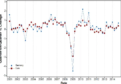
The GDP (Gross Domestic Product) can be used as a good indicator when consid-ering the economic growth of a country. We define a recession as two consecutive periods of negative growth and there have been several periods of recession for the euro areab (see Figure 1). Since its establishment in 1999 the euro area has had several periods of financial crisis; however these have not always been reflected by the German economy.

a_{Thomson Reuters Datastream 5.0 (}_{thomsonreuters.com}_).

b_{Data source: ECB statistical Data Warehouse} _{http://www.ecb.europa.eu/stats/keyind/}

(28)

[image:28.595.92.507.106.396.2]

Figure 1: The time series shows the quarter-on-quarter volume growth of GDP and expen-diture components for Germany (shown in blue) and the euro area (shown in red).

(29)

years, despite continuing growth in the largest economies of the area – Germany and France. The latter period is often referred to as the European sovereign-debt crisis (or the euro zone crisis). It is important to note that a financial crisis in the euro area will affect countries at different times and the rate of recovery will vary depending on the state of the country’s economy prior to the crisis.

Germany is one of the most highly developed nations in the world and the German economy is the 5th largest national economy by GDP (at PPP exchange ratesc_{). As}

such it is the largest economy within the euro area and plays a dominant role not only in the European Union but also within world economics (Germany’s share of world trade (exports and imports) for 2014 was 7.2%d). It has invested in the emerging markets within Asia and also been influential in the expansion of the EU to include countries in Central and Eastern Europe. Its most important trading partners, based on their percentage share of overall exports, are France, USA, UK, Netherlands and in recent years PR of China (in 2014 the share of Germany’s overall exports to these countries were 9.0%, 8.5%, 7.4%, 6.5% and 6.6% respectivelyd._.)

The German economy is predominantly based on exports, with exports accounting for 45.7% of its GDP in 2014 (Germany was the 3rd largest importer and exporter in the world in 2014; see Table 1 for exports/imports as a percentage of GDP for other years). They focus on industrially produced goods and services (in 2013 machinery accounted for 18.3% of exports, motor vehicles and parts 16.6% and chemical goods 11.6%d_{). This means that the status of the exports market can be a significant}

factor for growth within the German economy. The euro is a weaker currency than

c_{www.cia.gov/library/publications/the-world-factbook/geos/gm.html.}

(30)

the Deutschmark and this can be positive for the German economy as it means that German exports are cheaper to overseas consumers. However, as the value of the euro increased through 2002 the German economy once again fell into recession (see Figure 1) with a possible factor being the undesirable exchange rate between the euro and major currencies affecting the export markets with the increased price of goods produced in Germany. The financial crisis 2007 - 2009 also had an effect on the export markets when a lack of orders and sales resulted in a severe fall in German exports from 2008 Q4 (in 2008 Germany was the 3rd largest exporter in the world). However, a weak euro can have a positive effect on the export market and thus on the German economy – a record high of 2.2% GDP growth was reported for the 2nd quarter of 2010 (Figure 1). As we can see from Figure 1 the quarter-on-quarter volume growth of GDP for 2012 Q1, Q2 and Q3 were 0.3%, 0.1% and 0.1% respectively, meaning that Germany avoided a further recession at this time, unlike other countries within the euro area (e.g. Greece, Spain and Cyprus).There were two consecutive periods of decrease for Germany in 2012 Q4 and 2013 Q1 (both quarters a decrease of 0.4%) however by 2013 Q2 there was an increase of 0.8% meaning that Germany had recovered from the recession, again unlike countries such as Greece and Cyprus (both countries suffered from a negative quarter-on-quarter volume growth of GDP until 2013 Q4 and 2014 Q4 respectively.)e

e_{ECB statistics. Year-on-Year volume growth of GDP and expenditure components: 2.4 Exports}

(31)

Exports Imports

[image:31.595.142.454.99.350.2]

Year Total Goods Services Total Goods Services 2000 30.9 26.6 4.3 30.6 23.6 7.0 2001 31.9 27.5 4.4 30.1 22.9 7.3 2002 32.6 27.7 4.9 28.2 21.3 6.9 2003 32.6 28.0 4.7 29.0 22.1 6.9 2004 35.5 30.3 5.2 30.4 23.5 6.9 2005 37.8 32.2 5.6 32.7 25.4 7.4 2006 41.2 35.2 6.0 35.9 28.5 7.5 2007 43.1 36.9 6.1 36.4 28.9 7.5 2008 43.5 37.1 6.4 37.5 29.9 7.7 2009 37.8 31.4 6.5 32.9 25.6 7.3 2010 42.3 35.6 6.6 37.1 29.4 7.7 2011 44.8 38.2 6.6 40.0 32.1 7.9 2012 45.9 39.1 6.9 40.0 31.9 8.2 2013 45.6 38.5 7.1 39.8 31.1 8.7 2014 45.7 38.6 7.1 39.1 30.6 8.5

Table 1: The table shows Germany’s exports and imports as a percentage of Gross Domestic Product (GDP). The data is taken from ‘German Foreign Trade in 2014’, a report by Germany’s Federal Ministry for Economic Affairs and Energy.

2.3 The DAX Index

This is the benchmark index for the German equity market, representing around 80% of the market capitalisation listed in Germany. Along with some general prerequi-sites which must be fulfilled for a company to be listed on the DAX (equities listed in the Prime Standard, continuously traded on Xetra with a widely held stock of at least 10% and a head office (or largest sales volume) in Germany) there are two main criteria that must be met based on turnover and market capitalization. Based on these two main criteria, the DAX members are reviewed annually in September for regular entry/exit and in March, June, September and December for fast entry/exit. The rules for these adjustments are outlined below, in order.f

Fast Exit (45/45) A company is removed from the DAX if it is no longer one of

f

(32)

the 45 largest companies according to two quantitative criteria: exchange turnover and market capitalisation, provided that an advancing company ranks 35 or above in both criteria.

Fast Entry (25/25)A company is recorded in the DAX if it is within the 25 largest companies according to both of the two quantitative criteria.

Regular Exit (40/40)A company is removed from the DAX if it is no longer one of the 40 largest companies according to the two criteria. (A non-index value but ranked at least 35 in two criteria.)

(33)

3 A Comparison of Correlation Based Networks

In this chapter we consider three methods for filtering pertinent information from a series of complex networks modelling the correlations between stock price returns of the DAX 30 blue chip stocks for the time period 2001 - 2014. The dataset, cre-ated from Thomson Reuters Datastreamg_{, consists of the closing prices, adjusted for}

dividends and splits, of the 30 stocks that form the DAX 30 for the time period between 2001 and 2014. This is a significant time period for the German economy as discussed in the previous section. Using the Thomson Reuters Datastream database and also the FNA platformh we create the visualisations of the correlation-based networks. These methods reduce the complete 30×30 correlation coefficient matrix to a simpler network structure consisting only of the most relevant edges. The cho-sen network structures include the Minimum Spanning Tree (MST), Asset Graph (AG) and the Planar Maximally Filtered Graph (PMFG). The resulting networks and the extracted information are analysed and compared, looking at the clusters, cliques and connectivity. We also consider two specific time periods: a period of crisis (October 2008 December 2008) and also a period of recovery (May 2010 -August 2010) where we discuss the possible underlying economic reasoning for some aspects of the network structures produced.

This chapter is organised as follows. The dataset is presented in Section 3.1. The network structures are discussed in Section 3.2: MSTs (Subsection 3.2.1), AGs (Sub-section 3.2.2) and PMFGs (Sub(Sub-section 3.2.3). The Dax 30 is analysed in Section 3.3 (a period of crisis in 3.3.1 and a period of recovery in 3.3.3). Finally a summary is

(34)

given in Section 3.4.

3.1 Data

We begin by taking the daily adjusted closing prices of the 30 stocks that form the DAX 30 for the time period between January 2001 and December 2014. The mem-bers of the DAX 30 can change as it is reviewed quarterly (see Section 2.3 for further details) and so we take the current 30 members for each time period considered.

Denoting the adjusted closing price of stock i on day t as Pi(t), we calculate the daily logarithmic returns of the stock prices Yi, as:

Yi(t) = lnPi(t)−lnPi(t−δt). (4)

[Bonanno et al. (2004)] and [Tumminello et al. (2007)] considered the affect that varying the time horizon, δt, has on the hierarchical organisation of stocks. For our work we use one trading day, setting δt = 1. To look at the affiliation between the price returns of stocksi andj we calculate the pair-wise correlation coefficient using Pearson product-moment correlation for all trading days in the time period:

ρij =

hYiYji − hYiihYji

q

(hY2

i i − hYii2)(hYj2i − hYji2)

(5)

(35)

of trading days per month) with an interval of 10 days chosen for simplicity. Note that the final window for each annual set will not necessarily contain 23 observations but will end with the last observation for that specific year. This technique gives us a smoother transition of the networks - although can be a compromise with the chance of error. Forn stocks, this results in an n×n matrix with all entries within the interval [-1, 1]. These end values correspond to total anti-correlation between stocks i and j and complete linear correlation between stocks i and j respectively.

ρij = 0 represents no correlation between stocks i and j.

As discussed, the DAX 30 is reviewed quarterly so members can be removed or added to the DAX 30 during certain time windows we consider. For consistency we remove the stocks that are not present throughout the entire time window resulting in some having 28 or 29 stocks rather than 30. For example, 22nd September 2003 saw the regular exit of MLP and the entry of Continental (CON). When modelling the 2003 data we have a time window ranging from 10th September - 10th October 2003 which had 29 stocks as MLP and CON were both omitted. This is done automatically with FNA. In the following sections we consider various correlation based networks that have been presented in the literature as a way of filtering the most relevant data from the complete networks.

3.2 Network Structures

3.2.1 Minimum Spanning Tree (MST)

(36)

rel-evant connections from the correlation matrix and directly gives the subdominant ultrametric hierarchical arrangement of stocks. The stocks are clustered in a way that is entirely based on their correlations and Mantegna noted how this seems to be related to their economic sector.

Let G(V, E) be a connected, undirected graph, where V is the set of vertices and

E is the set of edges. A spanning tree S(V, E0) of the graph G is a subgraph that is a tree connecting all vertices of G, so if the number of vertices |V|= n then the number of edges |E0| = n−1. For a graph G(V, E) with positively weighted edges we can select the MST – a spanning tree where the sum of the edge weights is less than or equal to that of all other spanning trees. The MST is unique if all of the edge weights are distinct. Various algorithms have been proposed to construct a MST such as [Kruskal (1956)] and [Prim (1957)]. We have applied the Kruskal’s algorithm as this method is most common in the literature. To be able to construct a correaltion-based MST we need to define the distance between the vertices and the main method used in the literature is to construct the network using the Euclidean metric.

The distance between the stocks is defined so that the three axioms of a metric space are satisfied:

1. Positive Definiteness: For all p, q, r ∈ S we have d(p, q) ≥ 0 and (p, q) = 0⇔p=q;

2. Symmetry: d(p, q) = d(q, p);

(37)

whereS is a set and d is a metric on S.

We cannot construct a MST directly from the correlation coefficient matrix as using the correlations as distances would not satisfy these metric axioms – in particular, they do not satisfy the positive definiteness axiom as the correlations range from -1 to 1. Also a stock correlated with itself would give a correlation of 1 and not 0 as required by the first axiom. Furthermore, it is possible to have a high correlation between two stocks but for each of these stocks to have a low correlation with a third stock, which would thus not satisfy the third axiom. To transform the correlation matrix into a distance matrix, a metric function that incorporates the correlation coefficient and satisfies all axioms is needed. We have used a distance function used by [Mantegna (1999)] based on work by [Gower (1966)]:

d(i, j) =

q

2(1−ρij), (6)

where d(i, j) is the distance between stock i and stock j and ρij is the Pearson product-moment correlation coefficient (Eqn. 5) between stocki and stock j. With this distance function we create networks where the shorter the edge length between the vertices (i.e. stocks) the higher the correlation between them (see Appendix B for further details).

The 30×30 correlation coefficient matrix, C, is converted to a distance matrix,D, using the distance function shown in (Eqn. 6). Then(n−1)/2 = 435 distances from the upper triangular section ofD are then placed in ascending order, so that we can apply Kruskal’s algorithm.

(38)

data, with a time window from 5th February 2001 - 7th March 2001. The first nine of these ordered distances are shown in Table 2, along with the corresponding vertices:

Distance Vertices 0.515 SIE-IFX 0.591 EPC-IFX 0.625 SIE-EPC 0.643 DRB-DBK 0.755 EPC-DBK 0.781 SIE-DBK 0.782 EPC-DRB 0.794 SIE-DRB 0.807 DTE-DBK

Table 2: The first nine ordered distances for the MST construction from 5th February 2001 - 7th March 2001.

(39)

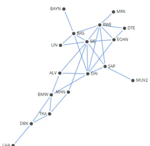
Figure 2: The first six vertices (labelled using the stock’s ticker symbol) and five edges of the MST extracted from data showing the correlation between the daily returns of the closing prices for the 30 members of the DAX 30 from 5th February 2001 - 7th March 2001.

(40)

The advantage of constructing this network compared to other methods (AG, PMFG) is that, when calculated in this way, the MST directly determines the subdominant ultrametric distance matrix. The axioms for an ultrametric space are similar to that of a metric space:

1. For all p, q,∈S we have u(p, q) = 0↔p=q;

2. u(p, q) = u(q, p);

3. u(p, r)≤ max[u(p, q), u(q, r)],

whereS is an ultrametric space and u is an associated distance function.

(41)

average ultrametric distances between vertices.

To illustrate the ultrametric distance between the stocks let us consider the sub-dominant ultrametric distance matrix, D<, for the first six vertices added to the MST from 5th February 2001 - 7th March 2001, as shown in Figure 2 and Table 2. Notice that there is an edge connecting vertices SIE-IFX, IFX-EPC and EPC-DBK with lengths 0.515, 0.591 and 0.755 respectively. Although there is no edge directly connecting vertices SIE-DBK there is a unique path connecting the two vertices (T(V, E) is a tree ⇔there is exactly one path between any 2 verticesu, v ∈V). The Euclidean distance between these vertices would be the total sum of the lengths of each edge in this path (i.e. 0.515 + 0.591 + 0.755 = 1.861). The ultrametric distance would be the max length of all edges in the unique path between the vertices (i.e. Max[0.515, 0.591, 0.755] = 0.755).

(42)

SIE IFX EPC DBK DRB DTE SIE 0 0.515 0.591 0.755 0.755 0.807 IFX 0.515 0 0.591 0.755 0.755 0.807 EPC 0.591 0.591 0 0.755 0.755 0.807 DBK 0.755 0.755 0.755 0 0.643 0.807 DRB 0.755 0.755 0.755 0.643 0 0.807 DTE 0.807 0.807 0.807 0.807 0.807 0

Table 3: The table shows the ultrametric distances between the first six vertices added to the MST extracted from data showing the correlation between the daily returns of the closing prices for the 30 members of the DAX 30 from 5th February 2001 - 7th March 2001, with the stocks labelled using their ticker symbols.

As stated above, stocks with the same ultrametric distances to other stocks can be clustered together. For example, SIE and IFX would form a cluster closely linked with EPC. DRB and DBK would form a second cluster. This can be shown using a hierarchical tree; Figure 4 shows a hierarchical tree for the first six stocks.

(43)

3.2.2 Asset Graph (AG)

The Asset Graph (AG) was introduced by [Onnelaet al. (2003)] as a network simi-lar to the MST but as one that includes all of the strongest correlations. The time dependent graphGt₍_Vt_{, E}t_{) is constructed from either the} _n₍_n₋₁₎_/_{2 entries of the} upper or lower triangular section of the distance matrix,Dt_{. Note that the distance} matrix is calculated using the distance function in Eqn. (6). Then(n−1)/2 distances are placed in ascending order. As with the MST, the AG has n−1 edges however now the set of edges chosen are the n−1 smallest distances from the ordered list. With this selection the set of edgesEt are then−1 strongest correlations (as shorter distances correspond to stronger positive correlations) and are chosen regardless of whether or not they form cycles within the network. A similar approach to the AG is to create threshold networks. [Tseet al. (2010)] constructed a threshold network from closing price data on US stocks, using a winner-take-all approach. This method reduces the complete network to a less complex one by including an edge between two stock prices if their cross correlation is larger than a set threshold value. The complexity of the resulting network can be determined by varying this threshold value.

(44)

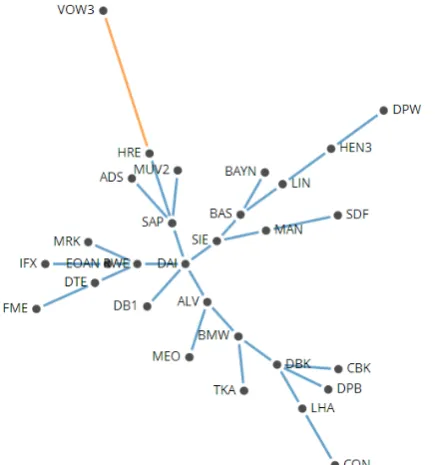
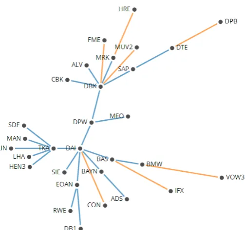
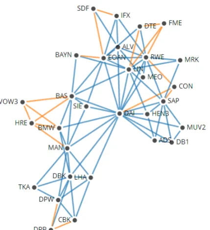
We return to the earlier worked example and look at the data from 5th February 2001 - 7th March 2001. Using the construction algorithm outlined above we create an AG with the 30 members of the DAX 30 during this time period. From Figure 5 we can see that six stocks have formed a 6-clique (SIE, DBK, DRB, DTE, EPC and IFX) and there are also three 3-cliques. Only 16 of the 30 vertices have been included in the AG.

Figure 5: The complete AG extracted from data showing the correlation between the daily returns of the closing prices for the 30 members of the DAX 30 from 5th February 2001 -7th March 2001. The vertices are labelled using the stock’s ticker symbol and have been coloured to highlight the clusters so they can be compared to the MST for the same time period (see Figure 3). Note that the lengths of the edges are not to scale.

(45)

sector; LIN produces industrial gases and so is classed as being in the industrial gases subsector. Thus the four stocks would form a cluster based on their sectors and subsectors. With the AGs from the same time period we see that it is BAYN that is the central vertex in this group – with a connection between BAYN and BAS in 48% of the networks (an average correlation of 0.7107). As well as producing industrial gases, one of the largest sectors of LIN is Linde Gas Therapeutics (pro-duction of medical gases). So LIN can also be seen to form a cluster with Fresenius (FRE), Fresenius Medical Care (FME) and Henkel (HEN3) (all of which belong to the pharmaceutical and health care sector). A similar example can be seen with the set of stocks BMW, Daimler (DAI) and Volkswagen (VOW3), all within the auto-mobile sector, and the networks for 2004 data. The MSTs show that at least two of these stocks are connected in 80% of the networks and all three are connected in 40% of the networks. The AGs for 2004 also show the strong correlations between these stocks, but they also identify that there are strong correlations between two insurance companies, Allianz (ALV) and Munich Re (MUV2), and BMW and DAI. This was something not shown with the MSTs.

(46)

Bank. In the 25 MSTs and AGs for 2003 SIE and DBK are connected in 56% of the MSTs and 72% of the AGs (an increase from the previous 2 years). Although we have not considered any social influences, e.g. companies having the same board members, the impact this can have on the networks has been discussed in [Halinen & Tornroos (1998)].

(47)

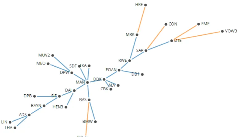
3.2.3 Planar Maximally Filtered Graph (PMFG)

The final network that we discuss in this section is the filtered graph proposed by [Tumminelloet al. (2005)] with particular focus on the planar filtered graph (PMFG – created when the graph is embedded into a surface with genus set equal to 0). The networks discussed so far are a severe form of data reduction, containing the minimum number of edges. The proposed filtered graphs allow us to choose how much information we filter from the complete network, so by increasing the genus of the surface we are able to construct a more complex network containing more edges. The PMFG is constructed in a similar way to the MST. For a graphG(V, E) with|V|=nand |E|=mall edges,e1, e2, . . . , em, from the upper triangular section of C are placed in descending order e(1), e(2), . . . , e(m). Select the first edge e(1) and

construct a graph with e(1) and the two vertices that it connects. Continue

select-ing the ordered edges and add them to the network structure only if the resultselect-ing network can be drawn on a planar surface without edges crossing. There are some tests for planarity based on Kuratowski’s theorem [Kuratowski (1930)] that a graph

G is planar if and only if it contains neither K5 nor K3,3 as a topological minor.

(For more detail on these and others see [Hopcroft & Tarjan (1974)]). The algorithm ends when all vertices v1, v2, . . . , vn are connected, using 3(n−2) edges (this is the maximum number of edges in a PMFG – for further details please see Subsection 4.1.2; Eqn. (8)).

(48)

stocks using the subdominant ultrametric distances in the direct way that we can with the MST. However, as the construction algorithm allows the inclusion of cycles the PMFG contains cliques, as with the AG, so we can extract further information from the network by analysing these cliques.

Looking specifically at the PMFG we consider 3- and 4-cliques, as the maximum number of elements that can form a clique is four. By considering the topology of the PMFG we can see that the basic structure (or motif) of the PMFG is a series of 3-cliques. Consider a sphere, a surface with g = 0. The PMFG separates the sphere into a sequence of triangular faces, with each vertex of the network belonging to a 3-clique. We can say that the PMFG is the triangulation of a sphere as the network consists entirely of 3-cliques (triangulation of a surface is a partition of that surface by triangles into facets). With our dataset of 30 stocks, we have a total of 30₃

= 4060 possible combinations of 3-cliques from each complete graph. By constructing the maximally filtered graph we considerably reduce the connectivity of the network leaving the most relevant cliques. (The possible structures of 3-cliques are discussed further in Section 4.2). We analyse the 4-cliques by showing the sectors that the four stocks belong to as well as the average correlation coefficient inside the clique, the range between the highest and lowest correlation coefficient in the clique and the standard deviation. Note that [Tumminello et al. (2005)] states the maximum number of 4-cliques formed by a PMFG isn−3 and we also prove this in Section 4.3.

(49)

three stocks are connected in 60% of the networks and actually form a 3-clique in 44% of the networks. We also considered the cluster of stocks in the automobile sector for the 2004 data. These clusters are also shown in the PMFGs, with the three stocks being connected in 72% of the networks and a 3-clique forming in 44% of the networks. Finally, the two stocks in the utilities sector, RWE and EOAN, were connected in a high proportion of the MSTs and AGs for 2009 and this was also the case with the PMFGs with a connection in 84% of the PMFGs for 2009.

Cliques also allow us to identify the most connected stocks so that they can not only be clustered but also separated into two sets: core and periphery. This can be done using the AG as, due to the construction algorithm, we often have clique components and unconnected vertices. However, the benefit of the PMFG is that, as it is a connected network, we have a better understanding of the relationships between the stocks that are not identified as being within the core.

(50)

3.3 Analysis of DAX 30

So far we have made comparisons between each of the network structures and dis-cussed their construction and the possible information we can extract. The filtered networks extract clusters of stocks from the complete networks which have high correlations between their return prices. These clusters often form between stocks that belong to the same economic sector and subsector with cross-sector clusters ap-pearing less frequently. There may be some economic reasons for these cross-sector clusters; however they could also be due to errors with the multiple simultaneous estimates made when creating the correlation matrices, such as type I errors (i.e. false positives – identifying a correlation when one does not exist). To this end, we have included the Bonferroni correction parameter when constructing the networks with FNA. For the Bonferroni correction, the familywise error rate (the probability of making one or more type I errors among all hypotheses when performing multiple tests) is set to the chosen level ofα (hereα = 0.05) and each individual test is per-formed at significance levelα∗ = _Mα whereMis the total number of tests performed. This method identifies edges in the network structures where the correlation may be classified as being statistically significant or insignificant.

We now discuss two specific time periods in more detail, discussing possible economic reasons for some of their features.

3.3.1 Period of Crisis

(51)

bil-lion, a later deal with an additionale15 billion was agreed on 5th October 2008) to prevent the collapse of Hypo Real Estate, the second largest commercial property lender. This was a sign of the economic problems in Germany – the GDP had de-clined 0.2% in the 2nd quarter of 2008 and a further 0.4% in the 3rd quarter of 2008 meaning as of 13th November 2008 the German economy was officially in a state of recession (see Figure 1).

(For the MSTs and AGs for this section please refer to Appendix C). The diam-eter of the MST increases as we move through the time period – this implies that the distances between the vertices is increasing and so the correlations are decreas-ing. There are some clusters that form – the two stocks from the utilities sector (RWE and EOAN) are strongly connected across the first four MSTs. Stocks in the FIRE (Finance, Insurance and Real Estate) sector (particularly the three banks Commerzbank (CBK), DBK and Deutsche Postbank (DPB)) are also strongly con-nected, in four of the five MSTs. However, in the final MST many of the edges that connect stocks from the FIRE sector to the tree are classified as insignificant – in-cluding CBK, DBK, DPB and MUV2. For the remaining MSTs the edges shown to be insignificant were rather predictable – mainly the edges connecting VOW3, HRE, CON and IFX to the networks for the period of crisis. The correlations that the test has found to be insignificant in the MST are the lower correlations that may have only been chosen to satisfy the construction algorithm. Some of the clusters identi-fied in the complete data set are not present in the MSTs – such as the automobile and the chemical cluster.

(52)

VOW3 has been previously discussed. CON and Hypo Real Estate (HRE) were both excluded from the DAX 30 on the basis of the fast-exit rule in December 2008 and similarly DPB and IFX were excluded in Q1 of 2009. The final two stocks that were not included are FME and Metro (MEO). We can see from the complete dataset that for some years FME does not cluster with any other stock and is included in very few AGs between 2002 and 2004 (actually it is not included in any AG for 2003). This could be because the company is fairly unique, being the only healthcare company included in DAX 30 at this point. Let us consider the correlations of the stocks that were included in the AGs. Across the series there is a decrease in correlations – the highest correlated pair falling from 0.9607 for the first AG to 0.8409. Although this is not a significantly large decrease if we consider that for the first AG the lowest correlated pair (the 29th and therefore last edge to be included) was 0.8631 we can see that there has been a decrease in the correlation throughout the complete graph. This supports what is shown by the increase in the diameter of the MSTs.

(53)

was identified as a special case and explained above (Subsection 3.2.2). PMFG Analysis Date Sto cks 4-Cliques Max.4-Cliques

4Sectors 3Sectors 2Sectors 1Sector

7 Oct - 6 Nov 2008 30 27 27 10 14 3 0

21 Oct - 20 Nov 2008 30 27 27 10 15 2 0

4 Nov - 4 Dec 2008 30 27 27 11 13 3 0

18 Nov - 18 Dec 2008 30 27 27 12 12 3 0

2 Dec - 31 Dec 2008 28 25 25 9 14 2 0

Table 4: The table shows the number of stocks for each time period, within the overall crisis period, the number of 4-cliques that formed, the maximum number of 4-cliques possible for that time period and how many of the cliques were made up of stocks from 4 different economic sectors, 3 different sectors, 2 different sectors or all from the same economic sector.

Overall we can see a decrease in the average correlation within the 4-cliques – the highest and lowest averages for 7th October - 6th November were 0.9044 and 0.7821 respectively, whereas for 2nd December - 31st December the highest was 0.7967 and the lowest 0.4168. When considering the economic sectors that the stocks of the 4-cliques belong to we can see from Table 4 that there are many cliques where all four stocks are from a different sector. To further analyse the 4-cliques we compute a quantity hyi, as shown by [Tumminello et al. (2005)], to calculate the spread of the correlation among the stocks belonging to each clique (where ρij ≥ 0). hyi is the mean value of the disparity measurey(i) = P

j6=i[ ρij

si]

2 _{over the clique (where}_{i, j}

are elements of the clique and Si is the strength of element i). For a clique with all correlations shared evenly between the stocks within the clique hyi= 1

3. For the

(54)

4th November - 4th December and 18th November - 18th December there are three cliques that have hyi slightly higher than 0.34 (ranging from 0.341 to 0.365). Each of these cliques continued one of the seven stocks mentioned above that were omit-ted from all AGs for this overall time period. For the final PMFG for this time series (2nd December - 31st December) the value forhyiwas greater than 0.34 for 11 cliques. The highest value was 0.474 for a 4-clique formed with DTE, FME, MEO and VOW3. This PMFG is the only one for this time period where VOW3 has non-negative correlations; however they are very small in comparison to the others which would explain the higher mean disparity value.

If we consider the edges that have been classified as insignificant within the PMFG we can see that, as with the MST, it is mainly the edges connecting the vertices VOW3, HRE and IFX for the first networks in the series. However, as each vertex in the PMFG has a degree of at least 3 there were more edges that were classified as insignificant compared with the MST. The final PMFG in the series, representing data from 2nd December - 31st December 2008, actually has a larger number of edges classified as insignificant – with vertices from a range of sectors having all the edges connecting it to the remaining network being insignificant.

3.3.2 Case Study – Hypo Real Estate Holdings AG

(55)

Figure 6: Times series of the daily closing price, adjusted for dividends and splits between 1st September 2007 and 1st September 2009. The red markers indicate the individual days.

December 2005 - 21st December 2008. However, on 15th September 2008 Lehman Brothers (the 4th largest investment bank in US) filed for bankruptcy due to financial problems stemming from the US subprime mortgage crisis. The bankruptcy had an affect on international financial markets and was a contributing factor (combined with its acquisition of Depfa Bank in October 2007) to the liquidity shortage facing HRE by the end of September 2008.i In an attempt to prevent the collapse of HRE a e35 billion Government State aid plan was announced on 29th September 2008 to provide much needed liquidity. This is highlighted by the severe dip in Figure 6 where the closing price falls from e13.96 on 26th September 2008 down to e3.8 on 29th September 2008. Plans for further State aid were announced on 6th October 2008 and February 2009. We can see some rises and falls around these time periods in both graphs. HRE, however, was replaced as a DAX 30 member by Salzgitter AG (SZG) on 22nd December 2008.

(56)

3.3.3 Period of Recovery

The second time period between 7th May and 3rd August 2010 is considered a time of economic success for Germany. With the country officially out of recession in August 2009, there was a significant growth in the country’s exports and with that a 3.6% growth to their economy in 2010. The 2nd quarter of 2010 showed a record high in the GDP growth rate (2.2%) (see Figure 1).

(For the MSTs and AGs for this section please refer to Appendix D). For the AGs created for this time period the only stock that is not included is Merck (MRK). FME and FRE are only included in one AG where they form a separate compo-nent with only one edge between each vertex. These are the only three stocks in the pharmaceutical and healthcare supersector and, although we cannot comment on the performance of the companies based solely on the networks, we can say that their price returns do not appear to follow the same patterns as the other stocks. There are some companies and selected services that are known to be more resilient during periods of financial crisis and this includes those in the pharmaceuticals and health-care (Merck reported a record after-tax profit in 2007 and became a member of DAX 30. In 2008 they reported a 7.1% increase in total revenue and in particular an 11% increase in revenue for their pharmaceutical business sector. There was some con-tinued growth through 2009 and by 2010 both Merck and Fresenius Medical shares were considerable outperforming the DAXj_{). MEO is also only included in one AG}

and for the two time periods this is the only stock in the multiline retail subsector. The range from the largest to smallest correlation in the AGs increases across the time period and the correlations are generally not as high as in the previous time

j_{For further details on each company please refer to the annual reports published for each}

(57)

period.

The MSTs again show that the edges classified as being insignificant are fairly pre-dictable – mainly the edges connecting FRE, FME and MRK to the networks for the period of recovery. The MSTs show some clear clusters based on the economic sectors that the stocks belong to, particularly the automobile, chemical and FIRE sector.

PMFG Analysis

Date

Sto cks

4-Cliques

Max.4-Cliques

4Sectors 3Sectors 2Sectors 1Sector

7 May - 8 Jun 2010 30 24 27 7 15 2 0

21 May - 22 Jun 2010 29 23 26 7 12 4 0

4 Jun - 6 Jul 2010 29 16 26 7 7 2 0

18 Jun - 20 Jul 2010 29 26 26 12 13 1 0

2 Jul - 3 Aug 2010 30 27 27 7 17 3 0

Table 5: The table shows the number of stocks for each time period, within the overall recovery period, the number of 4-cliques that formed, the maximum number of 4-cliques possible for that time period and how many of the cliques were made up of stocks from 4 different economic sectors, 3 different sectors, 2 different sectors or all from the same economic sector.

(58)

the average correlations for the 4-cliques were generally lower for the second time period when compared to those of the first. If we compare the values calculated for hyi to the values calculated in the first time period we see that there are even fewer cliques that have hyi greater than 0.333, with the highest value being 0.355. There are 13 cliques for the whole time series that have hyi higher than 0.34, and of these all but five contain one or more of MEO, FME, FRE or MRK which have been omitted from, or shown in only one, AG for this time period.

[Tumminello et al. (2005)] used a similar 4-clique analysis to investigate 100 US stocks from January 1995 to December 1998. The total number of 4-cliques formed was 97, and of these 31 had all four stocks in the same economic sector and 22 had three in the same economic sector. Our 4-clique analysis actually showed that it was more likely for a 4-clique to form with each stock in a different sector or at most two stocks to be in the same sector. Possible reasons for this difference could be that the time periods considered here were not ‘average days’, as they were a period of crisis and of recovery, and also that the length of the time period’s were shorter. The German DAX 30 is also considerably smaller than the 100 US stocks considered by [Tumminello et al. (2005)].

(59)

in-significant. This could show that they are not highly correlated with other stocks with the network and have only been included to satisfy the construction algorithm. This supports what was shown with the AGs for the period of recovery.

Some of the correlations may be driven by another factor, such as markets moving up or down in general. To control for this we apply Principal Component Analysis (PCA). PCA identifies patterns in data and expresses data in a way to highlight these similarities so we can control the effect of common factors such as the market return. As PCA needs a complete dataset some vertices were omitted if they were not present throughout the whole time period i.e. for the period of crisis Beiersdorf (BEI), CON, HRE, SZG and TUI were omitted from the networks and for the period of recovery Heidelberg Cement (HEI) and SZG were omitted. When performing PCA with all components we found that there was very little difference between the result-ing networks and the original networks. However, followresult-ing [Laloux et al. (1999)], for a second analysis we removed the first and largest component as this most likely represented the variance due to the market return and also removed components greater than component 6 as less than 1.5% of the variance was explained by these components. These networks were slightly different to our original networks but this could be due to the missing vertices. They still supported the findings from our analysis.

3.4 Summary

(60)

prices for DAX 30 stocks. The minimum spanning tree reduces the complete net-work to the minimum connected structure and can be used to show the hierarchical clustering of the stocks. The clusters that form are likely to be between stocks in the same economic sector. The asset graph separates the complete network into compo-nents – generally complete cliques and unconnected vertices. The planar maximally filtered graph combines these two methods by showing some hierarchical clustering, as it will contain the corresponding MST and also highlight the most connected stocks, as with the AG.

(61)

4 Maximally Filtered Graphs

In this chapter, we consider maximally filtered graphs in more detail and consider the construction and possible representations of planar graphs.

As discussed in Chapter 3 one of the key properties of the AG, threshold networks and PMFG is that cliques can form between the vertices in the network which can highlight relationships. [Huanget al. (2009)] creates threshold networks to analyse the Chinese stock market using a correlation threshold value −1 ≤ θ ≤ 1 where θ

is the correlation coefficient between two stocks. They study the relationship be-tween the maximum clique, maximum independent set (a subset I ⊆ V such that the subgraph G(I) has no edges) and the threshold value θ. [Huang et al. (2009)] state that ‘the financial interpretation of the clique in the stock correlation network is that it defines the set of stocks whose price fluctuations exhibit a similar behaviour.’

(62)

for 3-cliques. Although we lack a formal proof, our investigations suggest that these

numbers are the maximal number of 4-cliques and 3-cliques, respectively, that can be

observed in a PMFG of ns elements.’ As well as looking at the average correlations within the cliques and whether the cliques are from one sector or cross-sector we also consider the ratio between the number of cliques that have formed to the maximum number of cliques that could form. For this, [Tumminello et al. (2005)] used the normalizing quantities that have been mentioned above. This chapter provides the formal proof that 3n−8 and n−4 are indeed the maximum numbers of 3-cliques and 4-cliques possible in a PMFG and also an alternative construction algorithm.

4.1 Relational Definitions and Notations

Here we introduce some key terminology that is needed for the proof. Let G be a planar graph, i.e. a graph that can be embedded in the plane in such a way that the

edges ofGwill only intersect at the end points (the vertices ofG). The planar graph divides the plane intofaces, with each face bound by a simple cycle ofG. The num-ber of edges in this boundary is the degree of the face. The planar representations of Gare all possible isomorphic embeddings of Gin the plane.

(63)

A chord is an edge connecting two vertices of a cycle, which is not included in the cycle itself. For a graph Pn, a cycle of length k (k ≥3) is called a k-cycle, denoted

Ck. A cycle C is a pure chord-cycle if the interior of C contains no vertices and all of the interior faces of C are triangles. If each of the cycles of four or more vertices within a graph has a chord then the graph is called a chordal graph. A wheel graph, denoted Wn, is a graph withn≥4 formed by connecting a single vertex to all other vertices of an (n−1)-cycle.

4.1.1 Diagonal Flips

Consider two triangular faces which share a common edge and form a quadrilateral, (see Figure 7). [Negami (1994)] defines a diagonal flip of an edge as replacing the existing common edge with a new edge between the other two vertices. A diagonal flip is only possible if the resulting quadrilateral does not contain any multiple edges.

(64)

4.1.2 Surface Triangles and Separating 3-Cycles

As a result of Kuratowski’s Theorem [Kuratowski (1930)], we know that the PMFG allows cliques up to a maximum size of four vertices (the maximum number consid-ered in this thesis). The 3-cliques can take the form of triangles on the surface (a pure chord-cycle of length 3 that forms a face of the PMFG) or aseparating 3-cycle (a 3-cycle where both the interior and exterior of C3 contain one or more vertices).

Figure 8 shows this in more detail.

Figure 8: This PMFG with 6 vertices highlights the two possible 3-cliques. Vertices A,C,D form a clique and they outline a triangle on the surface. Vertices A,B,E also form a 3-clique however they do not outline a surface triangle but rather the edges enclose 3 surface triangles which share common edges. A,B,E forms a separating 3-cycle.

The faces bounded by a cycle of edges are calledfinite faces whereas the unbounded face (ABC in Figure 8) is called the infinite face. As the PMFG is a triangulation of the sphere this unbounded infinite face will also form a triangle.

(65)

the maximum number of faces). To do this we use the Handshaking Lemma and Euler’s formula (see Appendix E). For the remaining of this section let G(V, E) be a simple, undirected, finite planar graph.

Proposition 1. Let G be a PMFG with n vertices, e edges and f faces. Then have

e= 3n−6 and f = 2n−4.

Proof. SinceG is planar and deg(vi)≥2,

f

X

i=1

deg(fi) = 2e.

SinceG is a triangulation, deg(fi) = 3⇒3f = 2e.

We can substitute into Euler’s formula and obtain the following,

n− 3

2f+f = 2

f = 2n−4 (7)

and similarly,

n−e+2 3e= 2

e = 3n−6. (8)

(66)

4.2 Representations of Each Maximal Planar Graph

In this section the various representations of planar graphs are presented, which are used to achieve the main results shown in Section 4.3.

Using the relationship between the number of edges and the sum of the vertex de-gree we can calculate the maximum sum of all vertex dede-grees for a PMFG with n

vertices. By considering all combinations of the possible degrees of each vertex we can see what embeddings would be possible and, from these, which would be planar graphs. The following worked example shows this more clearly.

Example 1. Take G(V, E) where |V| = 8 then we know e = 3n−6 = 18 and so

P8

i=1deg(vi) = 2e= 36.

Then each vertex can have a degree value from the set {3, 4, 5, 6, 7} due to the restrictions that each vertex can be joined to all other vertices at most once (the PMFG does not allow for multiple edges) and the degree of each vertex must be at least 3. From this set there are 27 possible combinations that would give the total degree sum of 36 and from these combinations 13 would produce a planar graph. Graphs that have the same combination of vertex degrees and are isomorphic to each other are known asplanar representations and they will have the same number of 3-cliques (denoted C3) and 4-cliques (denoted C4), (see Figure 9). It is possible

(67)

Figure 9: PMFGs with n = 8 and deg[vA, vB, vC, ..., vH]=[7, 5, 5, 5, 4, 4, 3, 3]. These

graphs are isomorphic and haveC3= 16 and C4 = 5.

Figure 10: Both graphs havedeg[vA, vB, vC, ..., vH]=[6, 6, 5, 5, 4, 4, 3, 3] however they are

not isomorphic and so are not planar representations of a single graph. Furthermore, they have different numbers ofC3 and C4 with the graph shown in Panel (a) having C3 = 16,

C4 = 5 and the graph shown in Panel (b) havingC3 = 14,C4= 2.

4.2.1 Standard Spherical Triangulation Form

We now consider how these different embeddings relate to each other using the idea of diagonal flips, as introduced by [Negami (1994)].

(68)

(1994)] generalised the result from [Wagner (1936)],

Theorem 1 (Negami, 1994). For any closed surface F2_{, there exists a positive}

integer N such that two triangulations G and G0 of F2 are equivalent to each other

under diagonal flips if |V(G)|=|V(G0)| ≥N.

In the case of the PMFG, the triangulation of the sphere,N = 4.

Lemma 1. Any maximal graph with n vertices, n ≥ 4, can be transformed to the standard spherical triangulation (or normal form), (see Figure 11), using a series of

diagonal flips.

(For proof please refer to [Ore (1967)], Chapter 1).

From n ≥ 4, the degrees of each vertex in the standard spherical triangulation are as follows:

deg[v1, v2, v3, v4, ..., vi, ..., vn−1, vn] = [n−1, n−1,4,4, ...,4, ...,3,3].

(69)

4.3 Main Results

4.3.1 Generating Maximal Planar Graphs

In 1891 Eberhard proposed a system in which a combination of a set of three opera-tions could generate all possible maximally (filtered) planar graphs. We begin with the complete graphK4 and then choose a generating operation, ϕ1, ϕ2, ϕ3, from the

operation set, Φ. Each generating operation adds a new vertex to the graph. This system is denoted ashK4; Φ = {ϕ1, ϕ2, ϕ3}i.

Forϕ1, ϕ2, ϕ3 begin by deleting all of the chords of a pure chord-cycleCkwith length