Scaling of morphogenetic patterns in continuous and discrete models

(1)

1

Scaling of morphogenetic patterns in

continuous and discrete models

THESIS SUBMITTED IN ACCORDANCE WITH THE REQUIREMENTS OF THE UNIVERSITY OF LIVERPOOL FOR THE DEGREE OF DOCTOR OF

PHILOSOPHY

BY

MANAN’IARIVO LOUIS RASOLONJANAHARY

(2)

2

Acknowledgments

Foremost, I would like to express my sincere gratitude to my supervisor Dr Bakhtier Vasiev without whom this thesis would not have been possible. He allowed me to work on this project. I really appreciate his support, guidance, patience and helps during my studies over the past three years.

My special thanks go to my family for their patience, support and encouragement throughout the duration of this project.

(3)

3

General Introduction

In biological systems, individuals which belong to the same species can have different sizes. However, the ratios between the different parts of their bodies remain the same for individuals of different sizes. For example, for fully developed organism with segmented structure (i.e. insects), the number of segment across the size range of the individuals does not change. This morphological scaling plays a major role in the development of the organism and it has been the object of biological studies (Cooke 1981, Day and Lawrence 2000, Parker 2011) and mathematical modelling (Othmer and Pate 1980, Gregor, Tank et al. 2007, Kerszberg and Wolpert 2007) for many decades. Such scaling involves adjusting intrinsic scale of spatial patterns of gene expression that are set up during the development to the size of the system (Umulis and Othmer 2013). On the biological side, the evidence of scaling has been demonstrated experimentally on various objects including embryos. (Spemann 1938, Gregor, Bialek et al. 2005). For example, a Xenopus embryo was physically cut into dorsal and ventral halves in experimental conditions. The dorsal half which contains the “Spemann organizer” developed into a small embryo with normal proportion (Spemann 1938). Similar experiments carried out for the case of the sea urchin embryo lead to a smaller size of individuals (Khaner 1993). Also for flies of different species, the number of stripes on their embryos during their development remains the same although they are of different sizes. These stripes, which are visible at an earlier stage of the embryonic development, correspond to the spatial pattern of gene expressions and are the origin of the segmented body of the flies (Jaeger, Surkova et al. 2004, Gregor, Bialek et al. 2005, Arias 2008). On the mathematical side, Turing introduced the term “morphogens” for protein which is a key factor for pattern formation and he derived a model involving morphogens in which spatial patterns arise under certain conditions. Since then, various mathematical models of pattern formations have been developed. For the diffusion-based models, the spatial patterns do not scale with size. For models using reaction-diffusion equations, (combination of diffusion and biochemical reactions) a characteristic length scale is determined by the diffusion constant and reaction rate. Thus, when the size of the embryo changes, the spacing of the patterning remains fixed. This means that solutions of mathematical models based on reaction-diffusion do not show scaling (Tomlin and Axelrod 2007).

(7)

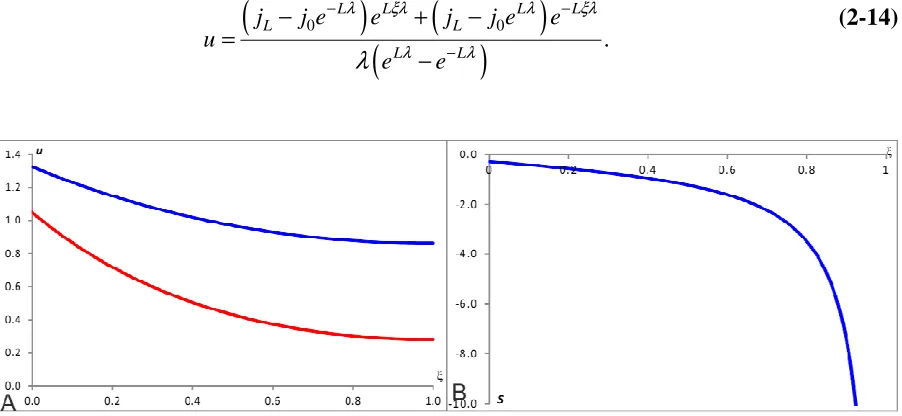
7

systems and demonstrate those using mathematical models. After a discussion on how the scaling is considered in a few continuous models, we introduce our definition of scaling. We apply our definition of scaling to analyse properties of concentration profiles arising in various continuous models. Upon analysis of these profiles, we introduce modifications of mathematical models, in particular, two famous continuous models (Turing and Fitzhugh-Nagumo) to achieve scaling of their solutions.

Following a presentation of continuous models, a discrete model of pattern formation based on a chain of logical elements (cellular automata) is also presented.This is more appropriate to represent the discreteness of biological systems with respect to their scaling properties: for a number of problems the issue of scaling doesn’t appear in the discrete formulation. This model has been developed to take account of local interactions between cells resulting into stationary pattern formation.

We conclude this thesis by comparing our results with results obtained on other models and with experimental data particularly related to the different stages of the development of the fly embryo.

The thesis is structured as follows:

Chapter 1 will discuss about the preliminary background. We will start with patterns in non-biological and non-biological systems. This is followed by how non-biological patterns were formed i.e. what mechanisms do we have for these pattern formations. Two of the main properties of biological patterns, which are robustness and scaling, will be briefly discussed in the next section. The mathematical aspects will follow with some examples of mathematical models. The final section will deal with a few continuous models.

Chapter 2 will concern the scaling of the continuous models. First, we begin with a simple one-variable model with a diffusion coefficient D and a decay coefficient k. We will investigate whether this model scales with the Dirichlet and Neumann boundary conditions. We consider two mechanisms of scaling of exponential profile. Then we consider scaling of the morphogen of the annihilation model. We consider the nuclear trapping model and active transport model.

(8)

8

the variant with three variables, we compute the solution for all variables and then we calculate the scaling factor for one of them. For the FHN model, we start with the two variables. Then, we move on to the three-variable FHN system. For this latter case, we have computed the scaling factor numerically.

(9)

9

Chapter 1 Introduction

1.1 Patterns in non-biological systems

Patterns are defined as orders embedded in randomness or apparent regularities (Chuong and Richardson 2009). They can appear in various systems and in different forms.

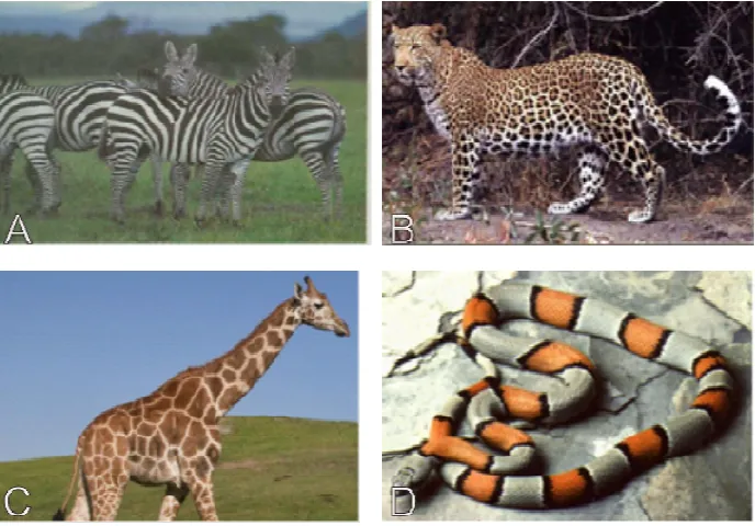
Living nature is one of the domains very rich in patterns. For instance in animal world, the zebra coat marking consists of a series of black and white stripes. The giraffe‘s neck has a spotted pattern. Some snakes have also a succession of multi colored ring along their body. Also, patterns can be found on some butterfly wings (Murray 2003). These are only a few examples but many more exist in animal world. Patterns can be found also in vegetal world. For instance, on a leaf, the veins exhibit a pattern along the midrib. On the fruit side, pattern is also shown on pineapple skin. Patterns can be seen as well on the flowers of sunflowers or white marguerite (Cowin 2000). Other examples can be found in vegetal world.

Figure 1-1: Pattern in natures.

A: Waves on the water surface – appear due to interplay of gravity and pressure when the dissipation of the mechanical energy is slow (low viscosity of water). B: Sand ripples appear

due to interplay of wind and gravity causing an instability in the shape of surface of the granular material (Yizhaq, J. Balmforth et al. 2004).

(10)

10

pattern can have a two dimensional form (succession of rising and failing of water level, for instance)(Rankine 1863, Bona, Colin et al. 2005). Steady three-dimensional patterns can exist as well at the surface of the water under certain conditions (constant density, irrational flow, inviscid fluid)(Bridges, Dias et al. 2001, Kerszberg and Wolpert 2007). In addition to the wind, a ship cruising at a constant speed on calm water can induce wave pattern known as the Kelvin wave pattern (Ohkusu and Iwashita 2004). Other forms of patterns exist at the surface of water.

For sand, the patterns have the appearance of ripples which can have wavelengths in the range of few centimetres to tens of meters and amplitudes from a few millimetres to a maximum of a few centimetres (Plater 1991, Hesp 1997). They can be observed in desert sand. The sand patterns are believed to be the result of the action of the wind on loose sand (Ball 2001). When the wind strength is large enough, the shear stress exerted by the wind on the sand surface lifts individual sand particles (Nishimori and Ouchi 1993). During their flight, the particles have approximately the velocity of the wind. During their impact with the sand surface, other sand particles are ejected (Sharp 1963, Walker 1981). For sufficiently large wind velocities, a cascade process happens and an entire population of saltating particles hopping on the sand surface emerges (Tsoar 1994). During strong winds, the layer of saltating particles can reach a thickness of more than 1 m (Ungar and Haff 1987, Livingstone, Wiggs et al. 2007). Sand ripple patterns can be found under water as well. For this case, the role of wind is played by the water (Yizhaq, J. Balmforth et al. 2004).

(11)

11

In fluid flow domain, the flow past a cylinder in two-dimensional domain exhibits a pattern which form depends on the Reynolds number. The Reynolds number is defined as the ratio of the product of the cylinder diameter and the undisturbed free-stream velocity flow and the viscosity of the fluid. When the free stream velocity is increased, a succession of vortices propagates away behind the cylinder (Van Dyke 1982). The flow past a cylinder is one of the most studied in aerodynamics and has many engineering applications (see Figure 1-2).

Figure 1-2: Flows past a circular cylinder.

A: Birth of vortices behind the cylinder for a Reynolds number of 2000. B: Two parallel rows of staggered vortices for Reynolds number of 150 (Van Dyke 1982).

1.2 Biological patterns

Biology is one of the domains rich in patterns and where the research on patterns has been done extensively. For biological systems, patterns exist in a wide range of size (from embryo to individual). They have emerged in the origin of life and its evolution (Hazen 2009). In this part, we deal with more details with some of these domains.

1.2.1 Skin patterns

(12)

12

[image:12.595.127.471.146.386.2]

patterns are shown to be generated by a single mechanism forming stripes, operating at different times in embryogenesis (Bard 1977). Turing has proposed a possible mechanism explaining how animals get their skin patterns (Turing 1952).

Figure 1-3: Examples of animal skin patterns.

A: Black and white stripes for the zebra. B: Spots for the leopard. C: Patches for the giraffe.

D: Periodic patterns (orange and grey) for the snake.

1.2.2 Shells of molluscs

(13)

13

shell patterns are given in (Meinhardt and Klingler 1987). Figure 1-4 shows an example of shells with patterns.

Figure 1-4:Stripes due to shell pigmentation occurring at regular basis. Upper: Stripes are parallel to the axis of the shell.

Lower: Stripes perpendicular to the axis of shell (Meinhardt 2009).

1.2.3 Segmentation of the fly embryo (Drosophila)

(14)

14

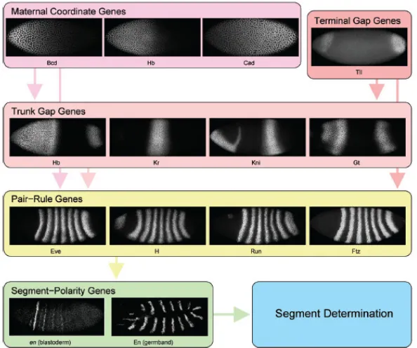
[image:14.595.150.447.243.491.2]

segment-polarity genes (wingless, hedgehog, engrailed)(Jack, Regulski et al. 1988, Small and Levine 1991). Segment polarity genes, in turn, are expressed in 14 narrow stripes shortly before gastrulation. These stripes constitute a segmental pre-pattern in that they determine the positions of morphological segment boundaries which form later in development (see Figure 1-5) (Perrimon and Mahowald 1987). The position and identity of body segments which take place during the embryogenesis are specified in the segmentation process (Jaeger 2009).

Figure 1-5: Hierarchy of Gene Control of Segmentation in Drosophila.

The patterning associated with the segmentation takes place in four levels: Concentration profiles of maternity genes (bicoid, caudal, etc.). These genes control the spatial patterns of

transcription of the gap genes. Spatial patterns of transcription of the gap genes (Hb, Kr, etc). The gap genes regulate each other and the next set of genes in the hierarchy, the

pair-rule genes (even-skipped, hairy, etc.). Pair-rule genes - form seven stripes of transcription around each embryo. Pair-rule genes determine the initial expression of segment polarity genes. Segment polarity genes - form fourteen stripes of transcription around each embryo

(Jaeger 2009).

(15)

(Flores-15

saaib and Courey 2000, Lin and Steward 2001). In the early embryo, the translocation of dorsal protein into ventral nuclei produces a gradient where the ventral cells with the most Dorsal protein become mesoderm (Umulis, O'Connor et al. 2008). The next higher portion becomes the neurogenic ectoderm. This is followed by the lateral and dorsal ectoderm (Francois, Solloway et al. 1994, Reeves, Trisnadi et al. 2012). The dorsalmost region becomes the amnioserosa (embryonic layer surrounding the embryo)(see Figure 1-6) (Gilbert 2010).

Figure 1-6: Dorso-ventral regions of early embryo.

In the early embryo, five distinct regions which are mesoderm, ventral ectoderm, lateral and dorsal ectoderm and amnioserosa appear. Left: Lateral view. Right: Transversal view

(Gilbert 2010).

1.3 Mechanisms of pattern formation

(16)

16

(Wolpert 2011). If the concentration of the morphogen is fixed at the source, then the distribution of its concentration at any point effectively provides the cells with positional information (Wolpert 1994).

Mechanisms of pattern formation have been classified into three categories (Salazar-Ciudad, Jernvall et al. 2003, Forgacs and Newman. 2005):

• autonomous mechanism in which cells enter into specific arrangements (patterns) without interaction,

• inductive mechanisms where cells interact with each other by secreting diffusible molecules. This leads to change in pattern by reciprocal or hierarchical alteration of cell phenotypes, and

• morphogenetic mechanisms where pattern changes by means of cell interactions that do not change cell states.

(17)

17

morphogen concentrations, which is the case if the movement is chemotactic and morphogens can act as chemotactic agents. These possibilities have recently been explored in studies combining mathematical modelling and experiments (Vasiev, Balter et al. 2010, Harrison, del Corral et al. 2011, Vasieva, Rasolonjanahary et al. 2013).

1.4 Symmetry and symmetry breaking in biological pattern

formation

Mathematically, symmetry is characterised by a group of transformations that leave certain features of a system unchanged (Mainzer 2005). This can be the invariance of the number of stripes on a fly embryo when the embryo size increases. In physical systems, symmetry can be seen as homogeneity (Golubitsky, Langford et al. 2003) or uniformity (Li and Bowerman 2010). It can be also characterised by the existence of different viewpoints from which the system appears the same (Anderson 1972). Also, the symmetry properties may be attributed to physical law (equations) or to physical objects or states (solutions)(Castellani 2002). Symmetry plays fundamental role in physics, for instance, in classical mechanics or quantum mechanics (Gross 1996).

Symmetry is a very important ingredient in a pattern formation model (spatial hidden symmetries in pattern formation). The application of the concept of symmetry has been extended by Turing in biology. In his famous paper in 1952 (Turing 1952), Turing showed that, in biology, pattern formation is governed by reaction-diffusion systems involving two chemical substances called morphogens. A spatially homogeneous distribution of these morphogens is unstable if one of them (activator) diffuses more slowly than the other (inhibitor). In this case, small stochastic concentration fluctuations are amplified, leading to a chemical instability (a “Turing instability”) and the formation of concentration gradients (or patterns)(Van der Gucht and Sykes 2009). These reaction-diffusion systems often possess symmetries. Specifically, the equations which describe them are often left unchanged by certain groups of transformations, such as reflection, translation or rotation.

(18)

18

Symmetry breaking does not imply that no symmetry is present, but rather that the situation is characterized by a lower symmetry than the original one. It refers to the situation in which solutions to the equations have less symmetry than the equations themselves. There are two types of symmetry breaking: spontaneous and explicit (Castellani 2002, Nogueira 2006, Li and Bowerman 2010). Spontaneous symmetry-breaking occurs when the laws or equations of a system are symmetrical but specific solutions do not respect the same symmetry. Here, spontaneous simply means endogenous to the dynamics of the system and not catalyzed by some exogenous input as in the case of explicit symmetry breaking. Explicit symmetry breaking means a situation where the dynamical equations are not invarivant under the symmetry group (Castellani 2002). It occurs when the rules governing a system are not manifestly invariant under the symmetry group considered. Also, in this case, the symmetry is broken by external objects.

1.5 Noise-induced pattern formations

Random fluctuations due to environmental effects are always present in natural systems. In addition to deterministic events which lead to pattern formation, these random fluctuations can also generate patterns. These pattern formations are explained as noise induced in the sense that they emerge as a consequence of the randomness of the system’s fluctuations. If the noise intensity is set to zero, the noise-induced patterns disappear and the homogeneous stable state is restored. These random drivers have often been related to a symmetry-breaking instability (Scarsoglio, Laio et al. 2011). They destabilise a homogenous (and, thus, symmetric) state of the system and determine a transition to an ordered phase, which exhibits a degree of spatial organisation.

In mathematical modelling of noise induced pattern formation, Gaussian white noise is usually adopted as it provides a reasonable representation of the random fluctuation of the real systems (the spatial and temporal scales of the Gaussian white noise are much shorter than the characteristic scales over which spatio-temporal dynamics of the field variable are evolving). At any point r(x, y) of the system, the spatio-temporal dynamics of the state variable is described by the following equation (Scarsoglio, Laio et al. 2011)

( )

( ) ( )

,

[ ]

_a

( )

, .

f g r t DL r t

t

ϕ

ϕ ϕ ξ ϕ ξ

∂

= + + +

(19)

19 This equation contains three components.

• The deterministic local dynamics f(ϕ) which tends to drive the field variable to a uniform steady state hence do not contribute to pattern formation,

• the noise components which consist of the multiplicative part g(ϕ)ξ(r, ϕ) and the additive part ξ_a(r, ϕ) maintain the dynamics away from the uniform steady state, and • the spatial coupling term represented by DL[ϕ] and which provides spatial coherence.

This spatial coupling is characterized by the operator L and its strength D.

Gaussian white noise with intensity s and zero mean is usually adopted as it provides a reasonable representation of the random fluctuation of the real systems (the spatial and temporal scales of the Gaussian white noise are much shorter than the characteristic scales over which spatio-temporal dynamics of the field variable are evolving) (Scarsoglio, Laio et al. 2011). For this Gaussian white noise, the correlation is given by

( ) (

r t, r t,

)

2s

(

r r

) (

t t

)

.

ξ ξ ′ ′ = δ − ′ δ − ′

Additive noise

In the case of additive noise, the model is represented by

[ ]

_a

( )

, .

a DL r t

t

ϕ

ϕ ϕ ξ

∂

= + +

∂

(20)

20

Multiplicative noise

For this case, the model is represented by

( )

( ) ( )

,

[ ]

.

f g r t DL

t

ϕ _ϕ _{ϕ ξ} _ϕ

∂

= + +

∂

In the case of multiplicative noise, the evolution depends on the value of the state variable ϕ. The cooperation between multiplicative noise and spatial coupling is based on two key actions: (i) the multiplicative random component temporarily destabilizes the homogeneous stable state, ϕ₀, of the underlying deterministic dynamics, and (ii) the spatial coupling acts during this instability, thereby generating and stabilizing a pattern (Scarsoglio, Laio et al. 2011). The key features of pattern formation induced by multiplicative noise are that for s

lower than a critical value s_c, the state variable ϕ experiences fluctuation about ϕ₀ but noise does not play any constructive role (Sanjuán 2012). For s greater than s_c, the spatial coupling exploits the initial instability of the system to generate ordered structures.

1.6 Robustness and scaling of biological patterns

(21)

21

Figure 1-7: Scalings of fly embryo and sea urchin.

A: Fly embryo of different sizes with the same number of stripes (segments). The upper and lower fly embryo have 485µm and 344µm respectively. Scaling was obtained by varying the lifetime of the Bicoid protein (Gregor, Bialek et al. 2005). B: At the two-cell stage, one has the development of the sea urchin. Hans Drieschs separated into two cells resulting that one

cell is dead and the other has given rise to a smaller sea urchin (Wolpert, Beddington et al. 1998).

Another key property of morphogen gradients is scaling. In Drosophila, development along the anterior-posterior axis is scaled with embryo length i.e. although individuals vary substantially in size, the proportions of different parts of the individuals remain the same, (see Figure 1-7)(Gregor, Bialek et al. 2005, Barkai and Ben-Zvi 2009). This adaptation of proportion (pattern) with size is termed as scaling. Experiments in scaling have been carried out towards the end of 19th_{century. In 1883, Whilhem Roux killed one of two cells in a frog} embryo and he found that the rest gave rise to only part of the embryo (Sander 1997). Hans Driesch, in 1891, he cut two cells of the sea urchin and each gave rise to full embryos (see Figure 1-7)(Kearl 2012). Four years later, Thomas Morgan repeated Roux’s experiment by removing one of two blastomere in a frog embryo and he found out that the amphibian could give rise a complete embryo from half an egg (Wolpert, Meyerowitz et al. 2001, Beetschen and Fischer 2004, De Robertis 2006).

1.7 Mathematical models for pattern formation

(22)

22

1.7.1 French Flag Model

The classical illustration of how a morphogen can provide positional information is given by the French Flag model suggested by Lewis Wolpert (Wolpert 1969). This model demonstrates how a simple linear concentration profile of a morphogen can set domains of cellular determination in an otherwise homogeneous tissue. The linear concentration profiles can form naturally in various settings. The simplest case is when the production and degradation of morphogen take place outside the tissue on its opposing sides and the morphogen passively diffuses along the tissue from the side where it is produced to the side where it is degraded. Mathematically, the concentration of the morphogen in this system should obey the so-called Laplace’s equation with Dirichlet boundary conditions, which for a tissue represented by a one-dimensional domain of length L is given by the following mathematical formulation (Vasieva, Rasolonjanahary et al. 2013)(see Figure 1-8).

In this model, C represents the concentration of the morphogen, D is the diffusion coefficient and C₁ and C₂are the buffered concentrations of the morphogen outside the two sides of the tissue. For this model, the pattern depends on the level of concentration. This model does scale because if, for example, the size of tissue is doubled then the size of all domains of cellular determination which are defined by the threshold concentration values T₁and T₂will be also doubled.

Figure 1-8: Linear gradient in the French Flag model forms due to passive diffusion of the morphogen.

x₁ and x₂ have T₁ and T₂ for the threshold concentration values respectively. C is the concentration of morphogen, D is the diffusion coefficient, C₁ and C₂are the concentrations

(23)

23

1.7.2 Morphogen gradient in system with decay

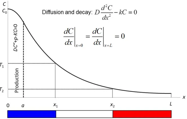
The linear shape shown in the French Flag model, in the previous section, is not confirmed by experimental observations. Most commonly measurements point to an exponential shape, as, for example, in the case of the transcriptional factor Bicoid in the fly embryo (Driever and Nusslein-Volhard 1988, Gregor, Wieschaus et al. 2007).Formation of the exponential profile can be shown mathematically under the assumption that the morphogen not only diffuses but also degrades inside the domain. The concentration of morphogen can be buffered on the boundaries of the tissue. Alternatively, we can assume that the tissue is isolated (no flows on the boundaries) and the production of the morphogen takes place in a restricted area inside the domain. These assumptions are perfectly reasonable for many studied objects. For example, the maternal Bicoid mRNA in fly embryo is localised in a small region on its apical side and the Bicoid protein produced in this region diffusively spreads and decays along the entire embryo. Stationary concentration of the morphogen in this system will satisfy the following equation (Vasieva, Rasolonjanahary et al. 2013)(Figure 1-9).

In this model, C and D have the same signification as previously, k represents the decay rate and p is the production of the protein in the apical side region of size a. When the area of the production is small, we can replace it by a boundary flux at x=0 (see proof in Appendix A). This figure does not scale because of the characteristic length of exponential profile. In other words, the distance required for the concentration to reduce by a certain factor (i.e. e-times), depends only on the diffusion coefficient, D, and the degradation rate, k, of the morphogen. For example, for the case shown in Figure 1-9,if we increase the size of the domain from L

to 2L then the sizes of blue and white sub-domains will not change while the red sub-domain will increase to cover all added L units of length (Vasieva, Rasolonjanahary et al. 2013). In an attempt to understand pattern formation in more depth, quantitative models of gradient formation have been developed. The addition of a degradation term with rate k to the Fick’s second law leads to the equation

2

2 .

C C

D kC

t x

∂ ∂

= −

∂ ∂

(24)

[image:24.595.135.464.74.283.2]

24

Figure 1-9:Exponential profile forms when the diffusion is combined with the decay.

C is the concentration of morphogen, D is the diffusion coefficient, x₁ and x₂ have T₁ and T₂ for the threshold concentration values respectively and C₀ is the concentration at x=0. We have production in the region between 0 and a with parameter p in the equation. And we

have Neumann boundary condition at both ends.

The steady state solution to this equation (1-1) with a production from localised source has an exponential form

( )

0 ,

x

C x =C e−λ

(1-2)

where C₀, in equation (1-2), is the concentration at the source boundary (x=0) and λ is the decay length given by λ=(D/k)1/2, i.e. the distance from source at which the concentration is reduced to a fraction 1/e of C₀. C₀ depends on the flux of molecules across the source boundary j₀, on the diffusion coefficient D and the degradation rate k as shown in (1-3) (Wartlick, Kicheva et al. 2009).

0

0 .

j C

Dk

= (1-3)

1.7.3 Turing’s Model

(25)

25

concentration (Turing 1952). His theory is based on the possibility of a stable state against perturbation, with absence of diffusion phenomenon to become unstable against perturbation in the presence of diffusion.

Turing’s pattern formation can be summarised as follows using two morphogen species, u

and v. The morphogen u is known as the activator because it is involved in the increase of its own production as well as to the production of the second morphogen v. The second morphogen v is called the inhibitor since it reduces the production rate of the activator and it also enforces its own degradation. For a 2D system (u, v), it is characterised by the set of ordinary differential equations.

( )

, , , ,

du

f u v dt

dv

g u v dt



=

 

 ₌



(1-4)

where f(u, v) and g(u, v) are non-linear functions. The equilibrium point (u, v)=(u₀, v₀) is solution of the LHS=0 of system (1-4). By adding a simple exponential type perturbation

t e v

u~,~∝ λ to (u₀, v₀), we will find λfrom the characteristic equation

0,

u v

f f

g g

λ

−

= −

where f_u, f_v, g_u and g_v are the derivatives with respect to u and v computed at (u₀, v₀). This gives

(

)

2

0.

u v u v v u

f g f g f g

λ

−

λ

+ + − =

From above, we have

(

_{) (}

2

₎

1,2 ,

2 4

u v

u v v u

f g

f g f g

λ = + ± + − −

In order to have stability, we need to request that Re λ<0. From the properties of the roots of quadratic equations, we have the following conditions

0,

u v

(26)

26 and

0.

u v v u

f g − f g > (1-6)

In the presence of diffusion phenomena, the set of previous ordinary differential equations (1-4) becomes

( )

, , , , u v u

D u f u v

t v

D v g u v

t ∂  = ∆ + _∂  ∂  ₌ _{∆ +} _∂  (1-7)

where D_u and D_v are the diffusion coefficients for u and v respectively. The equilibrium point (u, v)=(u₀, v₀) is solution of the LHS=0 of system (1-7). To study the effect of small perturbation, let

0

0 , .

u u u

v v v

= − = −

Linearising around (u₀, v₀), we get

, ,

u u v

v u v

u

D u uf vf

t v

D v ug vg

t ∂ = ∆ + + ∂ ∂ = ∆ + + ∂ (1-8)

where f_u, f_v, g_u and g_v are the derivatives with respect to u and v computed at (u₀, v₀). We are looking for solutions which can be represented as

( )

e , e , i i t i i i t i i i

u f x

v g x

λ λ

α

β

= =

∑

where α_iandβ_i are constants. Now the functions f_i(x) and g_i(x) can be represented as

( )

cos

( )

sin

( )

,

i i i i i i

(27)

27

where a_i and b_i are constants and k_i represents the wavelength. Assume that we have a function which goes from 0 to L and we want to extend it evenly i.e. the function is symmetric with respect the vertical axis. Then, in the solutions of f_i(x) and g_i(x), all the sine

functions will vanish. Therefore, the functions f_i(x) and g_i(x) can be written as

( )

cos

( )

,

i i i i

f x =g x =a k x

and the full solutions of u_and_v_{can be represented as}

e cos ,

e cos .

i i t i i t i i i u x L i v x L λ λ

π

α

π

β

  = _ _     = _ _  

∑

Any initial concentration profiles for both variables can be represented by above series. These series would represent solution of the system (1-8) if each pair of corresponding terms also satisfies this system. Therefore, we take one particular term from each of the above series

( )

1

cos e ,

t t u kx v kx λ λ

α

β

= =

and substitute them into equation (1-8), we obtain 2

1 1 1 1

2

1 1 1 1

,

.

u u v

v u v

k D f f

k D g g

α λ

α

β

β λ

β

α

β

= − + +

The above equations are linear in α1 and β1. Non-zero solutions only exist if the determinant of the matrix M is zero:

2

2 0.

u u v

u v v

f k D f

g g k D

λ

− −

= − −

This gives a quadratic equation in λ.

(

)

(

)

(

)

2 2 4 2

0.

u v u v u v u v v u u v v u

f g k D D k D D k f D g D f g f g

(28)

28

In order to investigate how diffusion phenomenon (D_u, D_v≠0) can destabilize the system, let’s consider the coefficient of

λ

and the constant term in (1-9). They are functions of k2_and denoted respectively as B(k2_{) and}_C₍_k2_).

B(k2₎_=f

u+gv−k2(Du+Dv), (1-10)

and

C(k2₎_=k4_D

uDv−k2(fuDv+gvDu)+fugv−fvgu. _(1-11)

Figure 1-10: Plot of C(k2_{) vs k}2_.

The condition (1-12) is satisfied for the blue curve but not satified for the green and red ones. The blue curve intersects the k2_{axis at} 2

1

k and k₂2. The instabilty occurs for k2_between 2

1

k and k₂2 i.e. one of the eigenvalues is positive. For the red and green curves, no Turing’s patterns occur (Murray 2003).

The function B(k2_{) is always negative for any value of}_k2_{according to (1-5). So, the only way} to have instability is that the function C(k2_{) is negative. To achieve that, we require that}

f_uD_v+g_vD_u>0. This is necessary but not sufficient condition. A sufficient condition is to have the minimum of C(k2_{) to be negative. The value of}_k2 _which_{gives this minimum value,}_C

min,

is solution of the derivative of C(k2_{) with respect to}_k2_i.e.

(

)

2

2k D D_u _v− f D_u _v+g D_v _u =0.

(29)

29

(

) (

2

)

2

0.

4 2

u v v u u v v u

min u v v u

u v u v

f D g D f D g D

C f g f g

D D D D

+ +

= − + − <

After rearranging, we obtain

(

)

2

. 4

u v v u

u v

f D g D

f g f g

D D

+

> − (1-12)

In other words, this condition leads to one of the eigenvalues to be positive. The range of k2 _{which corresponds to Turing’s instability is given by} 2 2 2

1 2

k <k <k where 2 1

k

and 2 2

k are zeros of C(k2_{). Their expressions are given by}

(

)

2

(

)

2 1,2

4

. 2

u v v u u v v u u v u v v u

u v

f D g D f D g D D D f g f g

k

D D

+ ± + − −

=

This case corresponding to the instability is represented by the blue curve in Figure 1-10. The values k₁ and k₂ are called the boundary wavenumbers. If k<k₁ or k>k₂, the perturbation due to the diffusion dies out without disturbing the homogeneous stable stationary state. The instability means that any noise with the right wavelength will be amplified by the system and leads to a spatial pattern with the matching wavelength. Turing’s instability (pattern) exists not only in biological systems but also in domains such as chemicals, physics, etc. In summary, the conditions to get the homogeneous stable stationary state to become instable with the presence of diffusion (diffusion driven instability) are as follows:

(

)

0, 0,

2 .

u v

u v v u

u v v u u v u v v u

f g

f g f g

f D g D D D f g f g

 ₊ _<



− >

 

+ > −



(1-13)

(30)

30

1.7.4 Fitzhugh-Nagumo model

The Fitzhugh-Nagumo model (FHN) belongs to a general class of reaction-diffusion equations (Dikansky 2005). This model has different variants and was originally developed as a generic model for signal propagation along a nerve fibre (Fitzhugh 1961). Its variant, which introduces the diffusion of the second variable, also serves as a generic model for morphogenetic pattern formations (Vasiev 2004). It is described by the following system (1-14) which have been obtained after time and space rescaling in order to allow the elimination of one of the diffusion coefficients and one of the kinetic rates

( )

, , , .

u

u f u v

t v

D v g u v

t

ε

∂



= ∆ +

_∂ 

∂

 _{= ∆ +} _∂



(1-14)

In the above system, D is the ratio of the diffusion coefficients and

ε is the ratio of the two

kinetic functions f(u, v) and g(u, v). The kinetic term in the first equation is defined by a cubic function f(u, v)=−k_uu(u−

α)(

u−1)−v (Nagumo, Arimoto et al. 1962) while in the second equation, it is simply represented by a linear function g(u, v)=k_vu−v. k_u and k_v represent constants related to the kinetic terms and α is a constant 0<α<<1 which is called “excitation threshold”.

Figure 1-11: Nullclines for three different dynamical regimes described by the FHN model.

The blue curve is the cubic nullcline f(u, v)=0 for activator. The green curve corresponds to the linear nullcline g(u, v)=0 for inhibitor. Three different type of system are shown. A: The origin is the only equilibrium point. This describes excitable system. B: The cubic nullcline has been shifted upward to give an oscillatory system. C: There are three equilibrium points. One can have either two unstable and one stable or two stable and one unstable. This system

(31)

31

Like in the Turing model, u and v represent the activator and the inhibitor respectively. Unlike the Turing model which patterns result from the difference of diffusion rates, the FHN patterns are based on the excitable dynamics from the reaction terms. By ignoring the diffusion terms, the above system has fixed points which are defined by the intersections of the two nullclines f(u, v)=0 and g(u, v)=0. According to the nature of the intersections, the kinetic system can be classified as excitable, bistable or oscillatory. For

α

≥0, one or two steady state solutions can be obtained. An oscillatory solution is obtained, for example, by adding an extra term to the function f(u, v) such that the nullcline is moved up. These are shown in Figure 1-11.

The model represented by the two equations above allows the understanding of pattern formation phenomena which occur in various chemical, physical and biological systems (Vasiev 2004). Different types of solutions can be obtained by changing the ratio of diffusion

D and ratio of kinetic rate ε.

Figure 1-12: Different 1-dimensional spatio-temporal patterns obtained from the solving of the scaled FHN equations according to the values of the parameters D and

εεεε

(Time:

vertical axis and space: horizontal axis).

All patterns were stimulated at the middle of the medium. A: Unstable patterns and the medium returns to the homogeneous state. B: Pulsating spot. C: Stationary spots. D: Self-replicating waves. E: The location of the domains, R₁, R₂, R₃_{and R}₄ on the (

ε

−1_{, D}

v) plane. D_v_{is acting as the ratio of diffusions. D}₁, D₂ and D₃_{specify the bifurcation parameters. The}

domain R₁ corresponds to the region with propagating waves, R₂_{corresponds to the region} where one a domain where the patterns are unstable and the medium as a rule returns to the

homogeneous state. R₃ corresponds to the domain where pulsating spots occur and R₄ corresponds to the domain where stationary spots arise (Vasiev 2004).

(32)

32

In Figure 1-12, four different scenarios are shown: propagating wave, vanishing spot, pulsating spots and stationary spots. They were obtained with different values of D. Propagating wave was obtained with D=1. D=2 is the case of the vanishing spot. Pulsating spots was simulated with D=3.2. All of these patterns can be classified into four regions which are shown in panel E of Figure 1-12.

1.8 Robustness of morphogen gradients

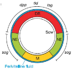
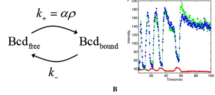
Mechanisms ensuring the robustness of dorso-ventral patterning in the Drosophila embryo against the changes in production rates (gene dosage) of involved proteins (BMP and Sog) have been studied both experimentally and theoretically in (Eldar, Dorfman et al. 2002). The analysis was based on detailed consideration of the dynamics of BMP, which is produced on the dorsal side of embryo, Sog, which is produced on the ventral side and inhibits BMP, and

BMP/Sog complex which is highly diffusive. The decay of Sog is mediated by Tolloid (Tld) - another protein whose concentration is assumed to be constant. Interactions between these substances can be graphically represented by the following:

,

, ,

.

b b

k k

Sog Scw Sog Scw

Sog Tld Tld

Sog Scw Tld Tld Scw

α γ −

+ ←→ −

+ ←→

− + ←→ +

Scw is the morphogen of interest. Sog inhibits the action of Scw by forming the complex

[image:32.595.222.370.541.683.2]

Sog−Scw. The protease Tld cleaves Sog.

Figure 1-13: Cross section of the Drosophila embryo.

(33)

33 These lead to the three reaction-diffusion equations:

[

]

2

_[

_]

_[

_][

_{] [ ][}

_]

_[

_]

,

BMP b b

Scw

D Scw k Sog Scw Tld Sog Scw k Sog Scw

t

λ

−

∂

= ∇ − + − + −

∂

[

]

2

_[

_]

_[

_][

_]

_[

_]

_{[ ][}

_]

,

S b b

Sog

D Sog k Sog Scw k Sog Scw Tld Sog

t −

α

∂

= ∇ − + − −

∂

[

]

2

_[

_]

_[

_][

_{] [ ][}

_]

_[

_]

,

C b b

Sog Scw

D Sog Scw k Sog Scw Tld Sog Scw k Sog Scw

t

λ

−

∂ −

= ∇ − + − − − −

∂

where D_BMP, D_S and D_C are respectively the diffusion rate constants for Sog, Scw and

Sog−Scw and k_b, k₋_b, α and λare reaction rate constants.

Figure 1-14: Non-robust and robust profiles of proteins Screw (Scw) using different values of boundary fluxes.

A: Non-robust profiles. The Sog profile is represented by the black dotted curve. The blue, red and green curves are three profiles of Scw with boundary fluxes values of 10, 5 and 2.5

respectively. And the yellow horizontal profile represents the sum Scw and its complex Sog

−

Scw. The values of the parameters are as follows: D_S=1, D_BMP=D_C=0.01, k_b=10, k₋_b=0.5,

λ

=2 and

α

=10. B: It is robust almost everywhere except when

ξ

=0.5. The values of

the parameters are as follows: D_S=1, D_BMP=0.01, D_C=10, k_b=120, k₋_b=1,

λ

=200 and

α

=1. The Sog profile is represented by the black dotted curve. The blue, red and green curves are

three profiles of Scw with boundary fluxes values of 10, 5 and 2.5 respectively. The dotted blue, red and green profiles represent the sum of Scw and its complex. And the yellow horizontal profile represents the sum Scw and it complex. C: The values of the parameters

are as follows: D_S=1, D_BMP=10−5_{, D}

C=1, kb=10, k−b=1,

λ

=1000 and

α

=1. The boundary fluxes of the dotted blue and continuous red profiles are 10and 5 respectively.

(34)

34

shown that high diffusion of the BMP/Sog complex enhances the dorso-ventral transportation of the BMP (the term used by authors is “shuttling”). Shuttling is obtained when the BMP

ligand, binding with the inhibitor, Sog, diffuses. This binding also facilitates the decay of

Sog. This mechanism has two advantages. First, it gives rise to a sharp gradient and second it allows robustness to fluctuation in gene dosage (Barkai and Shilo 2009, Haskel-Ittah, Ben-Zvi et al. 2012). A further modification of this model (Ben-Ben-Zvi, Shilo et al. 2008) with two additional equations describing the dynamics of BMP ligand Admp, which also forms a highly mobile complex with the BMP inhibitor, was used to demonstrate that a shuttling mechanism can also explain scaling of BMP gradient in Xenopus embryo.

1.9 Scaling of morphogen gradient

Scaling is a particular case of robustness. Scaling of morphogen gradients is the phenomenon which is persistently observed in experiments and represents one of the central problems in today’s mathematical biology. Space-scaling would mean that the characteristic length of morphogen gradient is proportional to the size of the tissue (see Figure 1-15).

Figure 1-15: Example of scaling with two patterns of different sizes.

The ratio x/L of two similar points (x₁ and x₂) of the individual to their respective lengths (L₁ and L₂) remains the same. In this figure x₁ is the distance between the blue and green stripes for the individual of length L₁and x₂ is the distance between the blue and green stripes for the

individual of length L₂.

There is scaling if, for the individuals of the same species, the ratio between the location of one characteristic point to the length of the individual remains unchanged from an individual to another

1 2

constant.

x x

L = L =

In general, if we call x the location of a characteristic point and L the length of the individual then, we have x/L=constant if we change from an individual to another.

x₁ x₂

(35)

35 constant.

x L =

We take the natural logarithm on both sides.

(

)

lnx−lnL=ln constant .

We take the derivative on both sides.

0, ,

dx dL

x L

dx dL

x L

− =

=

_S dx L_.

dL x

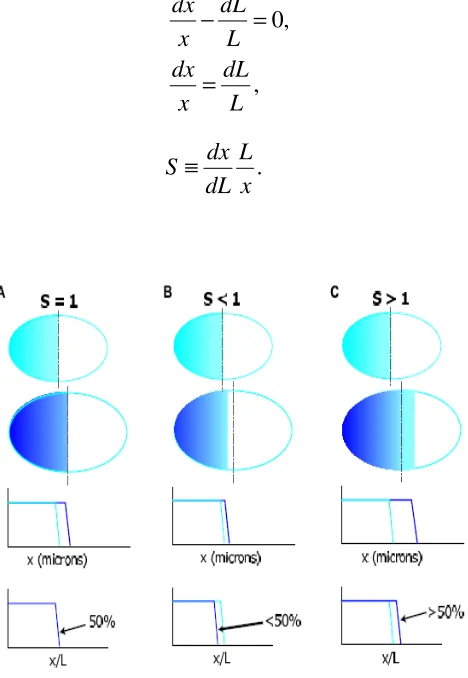
[image:35.595.183.417.224.563.2]

≡ (1-15)

Figure 1-16: Different scenarios associated with different values of the scaling factor S.

In the first case S=1. The domain which spans 50% of a small embryo will also span 50% of the bigger embryo. In the case of S<1, that is hypo-scaling, a domain which spans 50% of the smaller embryo will not expand enough in a bigger embryo. And in the case of hyper-scaling,

S>1, a domain which spans 50% of the smaller embryo will expand too much in a bigger embryo (De Lachapelle and Bergmann 2011).

(36)

36 1

.

C C L

S

L x x

− ∂ ∂ 

= − _ _ ∂  ∂ 

(1-16)

The above definition of scaling is generic and can be computed for any morphogen distribution C(x, t) (de Lachapelle and Bergmann 2010, De Lachapelle and Bergmann 2011). We see that this formula (1-16) depends on L and x. There is a problem with the above formula because at x=0, scaling does not occur since S=−∞. This allows us to introduce a better definition of scaling.

The above formula shows that the fluctuations in embryo length, dL/L, are exactly compensated by fluctuations in position, dx/x, implying perfectly conserved proportions. In this case (de Lachapelle and Bergmann 2010), considered that S=1 corresponds to perfect scaling. When S<1 and S>1, they refer to the terms hypo- and hyper-scaling, respectively (see Figure 1-16). Hypo-scaling means that there is not enough compensation for a change in embryo size, meaning that in a bigger embryo the absolute position is not shifted enough posteriorward to keep the correct proportions. Hyper-scaling is the tendency to overcompensate for a change in embryo size (de Lachapelle and Bergmann 2010).

1.9.1 Scaling in Annihilation model

Scaling of morphogen gradients can results from the non-linear interactions of involved morphogens. Assuming that the scaling of the Bicoid gradient is possible because Bicoid and Nanos, which are expressed in the opposite sides of the embryo, mutually affect their diffusion and/or degradation rate (Jaeger 2009). This leads to the annihilation model which is represented as

2 2 2

2

,

u u

v v

u u

D k uv

t x

v v

D k uv

t x

_∂ _∂

= −



_∂ _∂



∂ ∂



= −

_∂ _∂



(1-17)

where D_u and D_vare the diffusion coefficients and k_u and k_vspecify the decay rates. D_u, D_v, ku

and k_vare constants. The boundary conditions associated to this system (1-17) are:

(

)

(

)

(

)

(

)

0 0

0 , ,

0 , .

L L

u x u u x L u

v x v v x L v

= = = =

(37)

37

with u₀and v₀are the boundary values at x=0 and u_Land v_Lare the boundary values at x=L. We focus on stationary state of system (1-17).

2 2 2 2 0, 0. u u v v d u

D k uv

dx d v

D k uv

dx  − =     − =  (1-18)

As it is shown in the Appendix C, the relationship between variables u and v is given by the following:

(

0 0

)

0 0.

v u u v v u L u v L v u u v v u u v

x

k D u k D v k D u k D v k D u k D v k D u k D v

L

 

− = − − + _{ }+ −

 

We want to simplify the system (1-18) by considering D_u=D_v=D, k_u=k_v=k, u_L=v₀=0 and

v_L=u₀.

2

2 0,

d u

D kuv

dx − =

(1-19)

2

2 0,

d v

D kuv

dx − =

(1-20)

with the Dirichlet boundary conditions

(

)

(

)

(

)

(

)

0

0 , 0,

0 0, .

u x u u x L

v x v x L u

= = = =

For quantitative analysis, we will consider the sum and the difference of the two morphogens. First, we shall add equations (1-19) and (1-20).

(

)

2

2 2 0.

d u v

D kuv

dx

+

− =

(1-21)

Now, we subtract equation (1-20) from (1-19)

(

)

2

2 0.

d u v

D dx

−

(38)

38

Let s₊=u+v and s₋=u−v. Then the equations (1-21) and (1-22), in terms of s₊and s₋, will become

2 2

2 ,

d s k

uv D dx

+ ₌ (1-23)

2 2 0.

d s

dx

− ₌ (1-24)

The solutions of s₊ (see (1-23)) and s₋ (see (1-24)) are written as (see appendix C for full derivation).

0 1 2 ,

x s u L −   = _ − _   (1-25) 2

2 2 2 2

0 0

2 2 2 2 4

0

2 2 2 2

8 1 1 4 1 1

4 4

1 2 1 2 .

96

u L u L

L u

x x

s

L L L L

λ

+     − + + − + +         _ _ _ _     = +  −  −  −      (1-26)

The solution s₋ (see (1-25)) is a function of the relative position x/L, s₋= s₋(x/L) and therefore scales with the size of the medium. However, the solution s₊ (see (1-26)) does not scale since in addition to x/L it depends on the size, L, of the medium, s₊= s₊(x/L, L).

1.9.2 Scaling in the expansion-repression model

Most models of patterning formation by morphogen gradients do not exhibit the scaling property. (Ben-Zvi and Barkai 2010) show that the use of general feedback technology, in which the range of the morphogen gradient increases with the abundance of some molecule, whose production, in turn, is repressed by morphogen signalling. The derivation of their model is reproduced here for sake of clarity. It uses a single morphogen M secreted from a local source and diffuses in a naïve field of cells to establish a concentration gradient that peaks at the source. The distribution of this morphogen is governed by

[ ]

_{[ ]}

[ ]

_{[ ]}

[ ]

(

)

2 2 0 , 1 , 1 / M M E

E E h

M

D M M

t E

E

D E E

t _M _T

(39)

39

where D_M and D_E are the diffusion coefficients of M and E respectively,

α

_M and α_E are the degradation rates of M and E respectively,

β

_E is the production rate of E, h is the hill coefficient and T₀ is the threshold concentration.

Figure 1-17: Dynamics of the expansion-repression mechanism.

Initially, the morphogen and the expander diffuse from opposite ends. The morphogen repressed the expression of the expander when its level is above the threshold reference T_rep.

The expander which is diffusible and stable expands the morphogen gradient by increasing the diffusion and/or reducing the degradation rate. At a later time, the expander accumulates,

the gradient of the morphogen expands and the production domain of the expander shrinks. At steady state, the expander has accumulated and the gradient of the morphogen is wide enough to repress the production of the expander everywhere (Ben-Zvi and Barkai 2010).

It can be shown that the morphogen profile M(x) can be written as

M(x)=M(x/L, ρ),

where L is the size of the medium and ρ the morphogen production rate. This dependency of

the morphogen profile M(x) to the ratio x/L shows the scaling property of the expansion-repression model. Perfect scaling occurs if the profile M is insensitive to ρ. However, it has

been noticed that this dependency is typically small (Ben-Zvi and Barkai 2010). This model is not particularly good because the authors did not specify the natures of the morphogen M

Scaling of morphogenetic patterns in continuous and discrete models