size-structured integral projection model
.
White Rose Research Online URL for this paper:
http://eprints.whiterose.ac.uk/1394/
Article:
Childs, D.Z., Rees, M., Rose, K.E. et al. (2 more authors) (2003) Evolution of complex
flowering strategies: an age- and size-structured integral projection model. Proceedings of
the Royal Society B: Biological Sciences, 270 (1526). pp. 1829-1838. ISSN 1471-2954
https://doi.org/10.1098/rspb.2003.2399
[email protected] https://eprints.whiterose.ac.uk/ Reuse
Unless indicated otherwise, fulltext items are protected by copyright with all rights reserved. The copyright exception in section 29 of the Copyright, Designs and Patents Act 1988 allows the making of a single copy solely for the purpose of non-commercial research or private study within the limits of fair dealing. The publisher or other rights-holder may allow further reproduction and re-use of this version - refer to the White Rose Research Online record for this item. Where records identify the publisher as the copyright holder, users can verify any specific terms of use on the publisher’s website.
Takedown
If you consider content in White Rose Research Online to be in breach of UK law, please notify us by
Received18 February 2003
Accepted13 March 2003
Published online11 August 2003
Evolution of complex flowering strategies:
an age- and size-structured integral projection model
Dylan Z. Childs
1, Mark Rees
1*, Karen E. Rose
1, Peter J. Grubb
2and Stephen P. Ellner
31Department of Biological Sciences and NERC Centre for Population Biology, Imperial College, Silwood Park,
Ascot SL5 7PY, UK
2Department of Plant Sciences, University of Cambridge, Cambridge CB2 3EA, UK
3Department of Ecology and Evolutionary Biology, Corson Hall, Cornell University, Ithaca, NY 14853-2701, USA
We explore the evolution of delayed age- and size-dependent flowering in the monocarpic perennial
Carlina vulgaris, by extending the recently developed integral projection approach to include demographic
rates that depend on size andage. The parameterized model has excellent descriptive properties both in terms of the population size and in terms of the distributions of sizes within each age class. In Carlina the probability of flowering depends on both plant size and age. We use the parameterized model to predict this relationship, using the evolutionarily stable strategy (ESS) approach. Despite accurately predicting the mean size of flowering individuals, the model predicts a step-function relationship between the probability of flowering and plant size, which has no age component. When the variance of the flowering-threshold distribution is constrained to the observed value, the ESS flowering function contains an age component, but underpredicts the mean flowering size. An analytical approximation is used to explore the effect of variation in the flowering strategy on the ESS predictions. Elasticity analysis is used to partition the age-specific contributions to the finite rate of increase () of the survival–growth and fecundity components of the model. We calculate the adaptive landscape that defines the ESS and generate a fitness landscape for invading phenotypes in the presence of the observed flowering strategy. The implications of these results for the patterns of genetic diversity in the flowering strategy and for testing evolutionary models are discussed. Results proving the existence of a dominant eigenvalue and its associated eigenvectors in general size- and age-dependent integral projection models are presented.
Keywords:delayed reproduction; structured model; adaptive landscape
1. INTRODUCTION
Reproductive delays are a ubiquitous feature of plant and animal life cycles, and explaining why organisms defer reproduction is a classic problem in evolutionary biology (Cole 1954). The main benefits of early reproduction accrue through reductions in mortality and generation time (Cole 1954; Bell 1980). In general, reductions in mortality increase fitness, whereas reductions in generation time increase fitness only under certain circum-stances, and may have no effect on fitness in a density-regulated population (Mylius & Diekmann 1995). The costs of early reproduction are reduced fecundity and/or quality of offspring (Bell 1980).
In plants, the study of reproductive delays is compli-cated because plants vary continuously in size and there is enormous variation in growth between individuals. This means that the standard models, which assume growth is deterministic, perform poorly when applied to plants (Rees et al. 1999, 2000). To overcome these problems, previous studies have used analytical approximations, dynamic-state variable models or computationally expens-ive individual-based models (Kachi & Hirose 1985; de
Jonget al.1989; Wesselinghet al.1997; Reeset al.1999,
2000; Roseet al. 2002). Clearly, a mathematical
frame-*Author for correspondence ([email protected]).
Proc. R. Soc. Lond.B (2003)270, 1829–1838 1829 2003 The Royal Society
DOI 10.1098/rspb.2003.2399
work that allows (i) individuals to vary continuously in size and (ii) variation in growth is required. Integral projection models allow both these essential features of plant popu-lations to be modelled in an elegant framework, which is easily parameterized using standard demographic data. When combined with methods for calculating measures of population growth, such as the net reproductive rate (R0)
and the finite rate of increase (), and ideas from evol-utionary demography, this approach provides a powerful set of tools for exploring reproductive decisions in biologi-cally realistic models (Cochran & Ellner 1992; Mylius & Diekmann 1995; Caswell 2001).
The integral projection model was introduced by Eas-terlinget al. (2000) and subsequently developed for use in studying monocarpic plants by Rees & Rose (2002). The model eliminates the need to divide data into discrete classes, without requiring any extra biological assumptions (Easterling et al. 2000). Integral projection models have many properties in common with matrix models; for example, they allow the calculation of the stable size distri-bution, the population growth rate, and the sensitivities and elasticities of.
datasets are available, the probability of flowering is determined by a plant’s size and age (Klinkhamer et al. 1987; Reeset al. 1999; Roseet al. 2002). This is parti-cularly puzzling in species such as Carlina vulgariswhere all other demographic transitions are independent of plant age (Rose et al. 2002). Under these circumstances, the pay-off from flowering does not change as plants grow older and so the probability of flowering should not be influenced by plant age. Rose et al. (2002) suggest that under these circumstances age-dependent flowering might evolve because of temporal variation in mortality, because the population is part of a metapopulation or as a way of fine-tuning the flowering strategy. Additionally Reeset al. (2000) show, using a dynamic-state variable approach, that, when there is a finite time horizon (a maximum age), resulting from successional change or senescence, then there are fewer opportunities for growth as plants get older, and this selects for smaller sizes at flowering in old plants.
We present an extension to the integral projection approach allowing demographic transitions to depend on a plant’s sizeandage. We first outline the construction of integral projection models for monocarpic plants with size-dependent and age-dependent demographic rates, and numerical methods for analysing them. The results of Easterling (1998), proving the existence of a dominant eigenvalue and associated eigenvectors, are then extended to cover general size- and age-dependent integral projec-tion models. We then summarize the size- and age-dependent demography ofC. vulgarisand use this to con-struct a size- and age-con-structured integral projection model. Using methods from evolutionary demography, we ana-lyse the models to determine the evolutionarily stable flowering strategy under a variety of constraints (Mylius & Diekmann 1995).
2. MATERIAL AND METHODS
The integral projection model can be used to describe how a continuously size-structured population changes over discrete time (Easterling et al. 2000). The state of the population is described by a probability density function, n(x,t), which can intuitively be thought of as the proportion of individuals of size
xat timet. The integral projection model for the proportion of individuals of size y at timet⫹1, 1 year later, is then given by
n(y,t⫹1)=
冕
⍀[p(x,y)⫹ f(x,y)]n(x,t)dx
=
冕
⍀k(y,x)n(x,t)dx. (2.1)
wherek(y,x), known as the kernel, describes all possible tran-sitions from sizexto size y, including births. The integration is over the set of all possible sizes,⍀. The kernel is composed of two parts, a fecundity function,f(x,y), and a survival–growth function,p(x,y). To extend the model to include size- and age-dependent demography we definena(y,t) to be the probability
density function for individuals of size y and age ain yeart. The integral projection model then becomes
n0(y,t⫹1)=
冘
ma=0
冕
⍀fa(x,y)na(x,t)dx a=0,
na(y,t⫹1)=
冕
⍀pa⫺1(x,y)na⫺1(x,t)dx a⬎0,
(2.2)
Proc. R. Soc. Lond.B (2003)
wherefa(x,y) is the fecundity function, pa(x,y) is the survival–
growth function of plants of size x and age a, and m is the maximum plant age. These functions are referred to collectively as the kernel component functions. For a numerical solution, it is convenient to write the model in matrix form, which is given by
n(y,t⫹1)=
冕
⍀K n(x,t)dx, (2.3)
whereKis the matrix
K=
冢
f0(x,y) f1(x,y) % fm⫺1(x,y) fm(x,y)
p0(x,y) 0 0 0
0 p1(x,y) 0 0
哻
0 0 pm⫺1(x,y) 0
冣
(2.4)
andn(y,t)=(n0(y,t),n1(y,t),...,nm(y,t))T. To solve these models
we use numerical integration methods (Easterlinget al.2000). If each component function is evaluated at q equally spaced quadrature mesh points, yi, and w is the quadrature weight
(difference between theyis), we can then approximate equation
(2.3) as
n(t⫹1)=K˜Dn(t), (2.5)
wheren(t)=(n0(y0,t),...,n0(yq,t),...,nm(y0,t),...,nm(yq,t))T,
K˜ =
冢
f0(yi,yj) f1(yi,yj) % fm⫺1(yi,yj) fm(yi,yj)
p0(yi,yj) 0 0 0
0 p1(yi,yj) 0 0
哻
0 0 pm⫺1(yi,yj) 0
冣
(2.6)
andD=diag(w). TheK˜Dmatrix has the same form as Good-man’s transition matrix, the properties of which have been care-fully analysed (Goodman 1969; Law 1983). In Appendix A we prove that, under biologically reasonable assumptions, the model (equation (2.2)) has a dominant eigenvalue,, that is positive and strictly exceeds all others, and, when growing at a constant rate,, the population settles to a stable size–age distri-bution, which is given by the right-hand dominant eigenvector. To calculateR0, which is required for the evolutionary calcu-lations, the general methods described in Caswell (2001) can be used. However, a considerable saving in computer time and memory can be achieved by collapsing theK˜Dmatrix to a Leslie matrix. The key assumption required to collapse theK˜Dmatrix is that the probability distribution of offspring sizes is inde-pendent of adult size and age (Law & Edley 1990; see Appendix A). We can then construct a Leslie matrix, the eigenvalues of which are equal to those ofK˜D, and calculateR0using the stan-dard age-based formula.
To apply the model we must specify the dependence of sur-vival, growth and fecundity on size and age. We will present the equations forC. vulgaris, which has only size-and age-depen-dent flowering, but it is straightforward to extend the approach to include size and age dependence of other demographic tran-sitions. Specifically, we will write the fecundity function as
fa(x,y)=pes(x)pf,a(x)fn(x)fd(x,y), (2.7)
Modelling complex flowering strategies D. Z. Childs and others 1831
probability of survival of an individual of sizex, pf,a(x) is the
probability that an individual of sizex and ageaflowers,fn(x) is the number of seeds produced, andfd(x,y) is the probability distribution of offspring size, y, for an individual of sizex. The survival–growth function is given by
pa(x,y)=s(x)[1⫺pf,a(x)]g(x,y), (2.8)
whereg(x,y) is the probability of an individual of sizexgrowing to sizey. The probability of flowering,pf,a(x), enters the survival
function because reproduction is fatal in monocarpic species. To compare the model predictions with field data, we calcu-late the stable flowering-size distribution,(y), using
(y)=
冘
ma=0
s(y)pf,a(y)a(y)
冘
ma=0
冕
⍀s(y)pf,a(y)a(y)dy
, (2.9)
wherea(y) is the stable size–age distribution.
(a) Population biology ofC. vulgaris
Carlina vulgaris, a monocarpic thistle of base-rich soils (mainly found on limestone or calcareous sand), is native to a wide area in western, central and eastern Europe, and has been introduced to North America and New Zealand. Under very favourable growing conditions, Carlina individuals can flower in their second year (Klinkhamer et al. 1991, 1996; Reeset al. 2000) but, more commonly, reproduction is delayed by at least one more year. Previous studies in The Netherlands (Klinkhameret al.1991, 1996) have shown that the probability of flowering is related to plant size and not to age; however, in the UK the probability of flowering is related to both plant size and age (Roseet al.2002). Flowering occurs between June and August, and the seeds are retained in the flower heads until they are dispersed during dry sunny days in late autumn, winter or spring (P. J. Grubb, unpublished data). Seeds germinate from April to June, and there is little evidence of a persistent seed bank (Eriksson & Eriksson 1997; de Jonget al.2000).
Detailed descriptions of the study site and methods of analysis are given in Roseet al. (2002). We briefly describe the main results that are relevant to this article. The study spanned 16 years, and during this time the fates of over 1400 individuals were followed. The length of the longest leaf was used to meas-ure plant size and in all analyses this was transformed using natural logarithms. Growth was strongly size-dependent and well described by a simple linear model:
L(t⫹1)=ag⫹bgL(t). (2.10)
Size this year predicted size next year (F1,507=667.52,
p⬍0.0001), but there was no significant effect of age (F1,507=0.32, p=0.576); the parameter values were
ag=1.21 (0.09) andbg=0.71 (0.03), where the standard error is given in parentheses. Generalized linear models of the prob-abilities of mortality and flowering were constructed assuming binomial errors and a logit link function (McCullagh & Nelder 1989). There was no effect on survival probability of plant size (2
1=0.98, p⬎0.30) or age (21=2.31, p⬎0.10); the para-meter value was logit(s(x))=0.34 (0.06). Plant size was the most important predictor of flowering (2
1=139.86, p⬍0.0001), with larger plants being more likely to flower than smaller ones. There was an additional effect of age (2
1=19.37, p⬍0.001), such that older plants were more likely to flower. The age effect was still significant (p⬍0.001) after fitting year effects and
[image:4.598.307.546.86.172.2]Proc. R. Soc. Lond.B (2003)
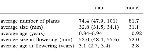
Table 1. Field data and model predictions.
(Values in parentheses are 95% confidence intervals.)
data model
average number of plants 74.4 (47.9, 101) 81.7 average size (mm) 32.8 (31.5, 34.1) 31.1 average age (years) 0.84–0.94 0.92 average size at flowering (mm) 52.0 (48.4, 55.6) 52.0 average age at flowering (years) 3.1 (2.7, 3.4) 2.8
allowing the size effect to be a smoothed function (generalized active model; Wood 2001). In the fitted logistic model for flowering, we will refer to the intercept, size slope and age slope as0,sanda, respectively; parameter values are given in table 2. To understand what the logistic regression means biologically it is necessary to distinguish between the threshold size for flowering, i.e. the size a plant must exceed in order to initiate flowering, and the size at flowering. These are different because (i) plants that flower are larger than the threshold size for flower-ing and (ii) there is variable growth between the time the decision to flower is made and the time at which flowering is recorded. However, we may interpret the fitted logistic model as a cumulative distribution function describing the threshold sizes for flowering. This implies that the probability density function of threshold sizes for flowering for plants of ageais described by a logistic distribution with mean and variance of ⫺(0⫹aa)/s and 2/32
s, respectively (Rees & Rose 2002). The mean size of flowering individuals observed in a population is obtained using equation (2.9). There was no relationship between this year’s seed production and the number of recruits in the following year, suggesting that the probability of recruit-ment is density dependent (Roseet al.2002); the mean number of recruits was 39.8 per year. This decoupling of recruitment from seed production was probably the result of establishment being limited by the available microsites: more seedlings are recruited when the turf was either short or opened up locally by trampling cattle (P. J. Grubb, personal observation). Two seed-sowing experiments, one in Sweden and one in Wales, support the idea that recruitment is dependent on disturbance (Greig-Smith & Sagar 1981; Lofgren et al.2000). Thus, if there are
Rrecruits into the population, the probability of establishment is given by
pe=
R
冘
ma=0
冕
⍀冕
⍀fa(x,y)na(x,t)dxdy
. (2.11)
Data were not available on the sizes of recruits derived from plants of different sizes, but evidence from other systems sug-gests a low maternal effect on recruit size (Weineret al.1997; Sletvold 2002), and so the distribution of offspring sizes was assumed to be independent of parental size; the parameter values were mean=3.09, variance=0.28—logarithmic scale.
3. RESULTS
(a) Analysis of the kernel
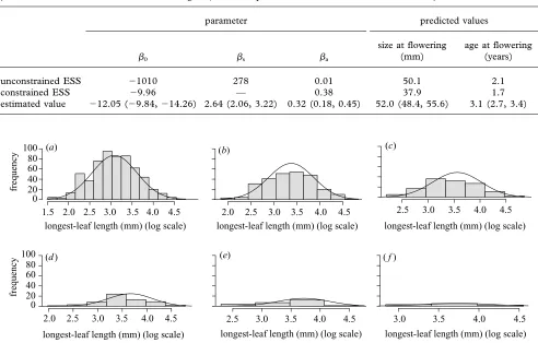
Table 2. Evolutionarily stable flowering strategy in terms of the parameters of the flowering function and the average size and age at flowering, assuming either that there are no constraints or that the slope of the flowering function,s, is constrained at its estimated value.
(For reference the estimated values are also given; values in parentheses are 95% confidence intervals.)
parameter predicted values
size at flowering age at flowering
0 s a (mm) (years)
unconstrained ESS ⫺1010 278 0.01 50.1 2.1
constrained ESS ⫺9.96 — 0.38 37.9 1.7
estimated value ⫺12.05 (⫺9.84,⫺14.26) 2.64 (2.06, 3.22) 0.32 (0.18, 0.45) 52.0 (48.4, 55.6) 3.1 (2.7, 3.4)
100 80 60 40 20 0
100 80 60 40 20 0
1.5 2.0 2.5 3.0 3.5 4.0 4.5 2.0 2.5 3.0 3.5 4.0 4.5
2.0 2.5 3.0 3.5 4.0 4.5 3.0 3.5 4.0 4.5
2.5 3.0 3.5 4.0 4.5
2.5 3.0 3.5 4.0 4.5
(a) (b) (c)
(d) (e) (f)
longest-leaf length (mm) (log scale) longest-leaf length (mm) (log scale)
frequency
frequency
longest-leaf length (mm) (log scale)
longest-leaf length (mm) (log scale) longest-leaf length (mm) (log scale) longest-leaf length (mm) (log scale)
Figure 1. Observed (filled bars) and predicted (lines) stable size–age distributions for ages 0–5 years, (a)–(f), respectively. The bar width in each histogram was chosen using a kernel density estimation routine to make the plots maximally informative.
We also calculated various measures of population size and age structure, using the methods outlined in Rees & Rose (2002), and, in all cases, the model predictions were in excellent agreement with the field data (table 1). As density dependence is explicitly modelled, we can calcu-late the equilibrium population size, and again there is excellent agreement between the model and the data (table 1).
(b) Evolution of the flowering strategy
To calculate the evolutionarily stable flowering strategy we need to specify not only how demographic rates vary with size and age but also where in the life cycle density dependence acts (Mylius & Diekmann 1995). InCarlina, the probability of seedling establishment is density depen-dent, while the effect of intraspecific competition is weak (Roseet al.2002). Under these conditions it can be shown that the evolutionarily stable strategy (ESS) maximizes the basic reproductive rate, R0 (Mylius & Diekmann 1995;
Rees & Rose 2002). We used a quasi-Newton algorithm to maximize R0 and so characterize the ESS. Given the
evolutionarily stable flowering strategy we then use equ-ation (2.9) to calculate the distribution of sizes at flower-ing.
Allowing all three parameters to vary, we find that the ESS tends towards a step function without an age compo-nent (table 2). Specifically, the variance of the
flowering-Proc. R. Soc. Lond.B (2003)
threshold distribution tends to zero as s→⬁ and
a→0. This matches our expectations for a
constant-environment model in which the key demographic processes of growth, survival and fecundity are all inde-pendent of age. The flowering-size threshold in this case (given by exp(⫺0/s)) tends to 37.8 mm, and the
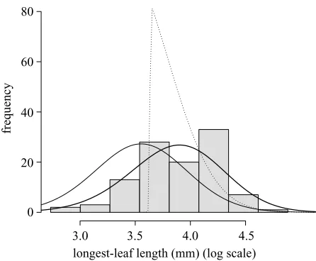
pre-dicted average size at flowering is not significantly differ-ent from the observed value (table 2). However, the variance in the distribution of flowering sizes is much smaller than that observed in the data (figure 2).
We also calculated the ESS assuming that the size-dependent slope of the flowering function,s, was fixed.
We use this constraint to prevent the ESS from being a step function. There are several reasons why it might be impossible for plants to achieve a step function: (i) there is variable growth between when the decision to flower is made and when plant size is measured; (ii) plant size may not be perfectly correlated with the threshold condition for flowering; and (iii) there may be genetic variation in the threshold condition. Withsconstrained the predicted
flowering strategy (0,a) is similar to the observed
strat-egy, although the predicted size at flowering is consider-ably smaller than that observed in the field (table 2). As expected, because s is fixed, the variance in the size at
flowering is similar to that observed in the field (figure 2). Interestingly, when we constrains, the predicted
Modelling complex flowering strategies D. Z. Childs and others 1833
80
60
40
20
0
3.0 3.5 4.0 4.5
longest-leaf length (mm) (log scale)
[image:6.598.58.281.59.243.2]frequency
Figure 2. Observed distribution of flowering sizes (filled bars) and predictions from the various models, calculated using equation (2.9). The bold line is the fitted model, the dotted line is from the unconstrained ESS model and the solid thin line is from the constrained ESS model.
(c) Analytical approximation
To understand how different aspects of Carlina’s demography influence the observed flowering size we extend the 1-year look-ahead approach described in Rees
et al.(2000). The approach derives a switch valueLs: on
average, plants with L(t)⬎Ls are expected to flower,
while plants withL(t)⬍Lsare expected to continue
grow-ing. The switch value is determined by equating expected seed production given the current size,Ls, with expected
seed production in the following year, taking growth and mortality into account. It should be noted that the approach is only approximate because it ignores opport-unities for growth more than 1 year ahead. In this system, the probability of survival is independent of size and age such that the survival function can be written as
s(x)=exp(⫺d0). (3.1)
Growth is described by equation (2.10) and seed pro-duction is given by
seed production=exp(A⫹BL(t)). (3.2)
Placing the component functions together we find that the switch value,Ls, satisfies the equation
冕
exp(A⫹B(Ls⫹ f))f(f)df=
冕冕
exp(⫺d0⫹A⫹B(ag⫹bg(Ls⫹ f))⫹ )f(f)f()dfd,(3.3)
where f(·) is the normal probability density function, f describes the between-individual variation in Ls, and
describes the variation around the growth function. Evalu-ating the integrals and solving forLswe find
Ls=
ag⫹B2/2
(1⫺bg)
⫺ d0
B(1⫺bg)
⫺
2
fB(1⫺bg)
2 , (3.4)
where2is the variance about the growth equation (2.10).
The first and second terms describe the effects of growth and mortality, respectively, on the mean switch size. The
Proc. R. Soc. Lond.B (2003)
first term is related to the arithmetic asymptotic average size; this is given by
l=ag⫹2/2
1⫺bg
. (3.5)
As expected, the switch value increases with increasing asymptotic size and decreases with increasing mortality. The dependence of the mean switch value,Ls, on variation
in the switching size is less intuitive: increasing variability around the mean switch size selects for smaller switch sizes,because the variance term,2
f, which arises because of nonlinear averaging, is always negative. There was excellent agreement between the unconstrained ESS flowering threshold size (37.8 mm), for which2
f =0, and the predicted switch value, 36.7 mm, calculated using equation (3.4). The 1 year look-ahead approach predicts a lower switch value because it ignores growth more than 1 year ahead; however, the discrepancy is small because of high size-independent mortality. Comparison of the two approaches in the constrained case is complicated because the ESS contains an age component. However, the 1 year look-ahead approach correctly predicts that variance in the threshold condition selects for smaller flowering sizes.
(d) Fitness and adaptive landscapes
In this system density dependence acts on the recruit-ment stage and so evolution maximizes R0. A plot ofR0
against the flowering strategy can be interpreted as an ‘adaptive landscape’ in the classical sense (Wright 1931). Its topography is unaltered by the presence of a particular resident, and an ESS is defined by a local maximum. At equilibrium R0==1 and so represents the rate of
invasion of new strategies into the resident population, such that the surface forrepresents a fitness landscape. Its topography describes the strengths of selection acting on alternative strategies (Metz et al. 1992; Rand et al. 1994). We computed the adaptive and fitness landscapes for a wide range of 0 and a, assuming s was fixed
(figure 3). When interpreting these graphs it must be remembered that as0gets smaller (more negative) so the
size at flowering increases. The adaptive landscape shows that the ESS lies within the 95% confidence envelope for the estimated parameters. Moving from left to right across the adaptive landscape we see a dramatic increase in the performance of the flowering strategy; this reaches a maximum then declines to a plateau where all strategies have equalR0. Clearly, flowering at sizes much larger than
the ESS results in a dramatic loss of fitness. This is a consequence of high size-independent mortality (ca. 40% of plants die each year). The plateau in the adaptive land-scape, corresponding to large values of0, occurs because
all plants flower in their first year, and so have equal per-formance (R0). Moving vertically across the adaptive
0.4 0.6
0.8
1.16
1.1
0.4 0.6
0.8
1
1.09
2
1
0
–1
–2
–30 –25 –20 –15 –10 –5 0 (a)
(b)
age slope,
a
β
intercept,β0 1
0.2
0.2
1.05
2
1
0
–1
–2
age slope,
a
[image:7.598.67.271.62.441.2]β
Figure 3. The (a) adaptive and (b) fitness landscapes for
Carlina, calculated assuming that the resident population uses the estimated flowering strategy. The large dot is the estimated flowering strategy, and the ellipse is the 95% confidence contour, calculated using the standard quadratic approximation to the likelihood—assuming that the likelihood is2-distributed with three degrees of freedom. The small dot is the ESS prediction assumingsis fixed.
(e) Sensitivities and elasticities
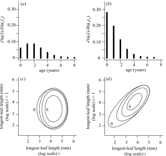
The standard approach for understanding how various parameters influence the fitness of rare mutants is to esti-mate the elasticities of mutant fitness (Caswell 2001). Elasticities can be used to measure the effect onof pro-portional changes infa(x,y) and pa(x,y) and can be com-puted using the methods described in Easterling et al. (2000) (see Appendix A). As elasticities sum to unity, this allows us to partition the contributions of fa(x,y) and pa(x,y) to of different age classes (figure 4a,b). This shows that the survival–growth function has a larger influ-ence onthan does the fecundity function (0.66 and 0.34, respectively), and that the largest contributions tocome from changes in the survival–growth function, pa(x,y), of young plants.
4. DISCUSSION
We have extended the integral projection modelling approach to include a discrete structuring variable such as
Proc. R. Soc. Lond.B (2003)
age, allowing us to explore the demography and evolution of size- and age-structured populations using a set of stan-dard numerical techniques. The analytical results (Appendix A) justify the numerical methods used and should prove useful in future studies where the distri-bution of offspring sizes depends on parental size or age. The ‘mixing at birth’ assumption is likely to be valid for a wide range of species, particularly when the size distri-bution of recruits is recorded several months after recruit-ment occurs (Weiner et al. 1997; Sletvold 2002). In contrast to age- and size-structured matrix models, where parameterization is difficult (Law 1983), extending an integral projection model to include the effects of age can be done by including age as an additional covariate when constructing the survivorship, growth or flowering func-tions. This means that a standard statistical test can be used to explore whether both size and age should be included in the model (Venables & Ripley 1997). Hence, this framework retains all of the power of traditional matrix models while being easy to parameterize.
The parameterized model provides an extremely accur-ate description of the number of individuals and the distri-bution of sizes within each age class, the distridistri-bution of flowering sizes, the average age at reproduction and the average population size. Despite this, the ESS predictions differ in either the mean or the variance from the observed distribution of flowering sizes. These discrepancies force us to conclude that important aspects of the selection pressures acting onCarlinaare not included in the model. The analyses presented by Roseet al.(2002) strongly sug-gest that temporal variation in demographic rates is a missing component of the selective environment. In this study, temporal variation in the intercept of the survival and growth functions was found to select for larger sizes at flowering. Curiously, the parameters of the constrained ESS are not significantly different from the estimated parameters of the flowering function, which suggests that one needs to be careful when comparing the predictions of evolutionary models with data, as different metrics may produce different results. Clearly, any satisfactory model needs to describe both the shape of the flowering function and the distribution of sizes at flowering, and we cannot assume that a model that is correct in one respect will be correct in the other.
Why does the flowering function contain an age-depen-dent term when the key demographic processes of growth and survival are independent of age? First, it must be acknowledged that the apparent age dependence could be an artefact of using an indirect measure of plant size, namely the length of the longest leaf. If older plants have larger tap roots for a given longest-leaf length, then the resources available for flowering to an older plant will be underestimated, resulting in an apparent increase in the probability of flowering with age. We know of no data on age-dependent resource allocation and therefore cannot discount this possibility, although Klinkhamer et al. (1987) found that longest-leaf length was the best predic-tor of total plant weight inCirsium vulgare, a monocarpic plant that also has size- and age-dependent flowering.
Modelling complex flowering strategies D. Z. Childs and others 1835
0.30
0.20
0.10
0
0 2 4 6 8
age (years)
2 3 4 5 6
0 2 4 6 8
age (years)
2 3 4 5 6
6 5 4 3 2
longest-leaf length (mm) (log scale) t
∂
ln(
fa
)
ln( )
/
∂
λ
longest-leaf length (mm)
(log scale)
t
+ 1
(a) (b)
(c) (d)
6 0
0
6
∂
ln(
pa
)
ln( )
/
∂
λ
longest-leaf length (mm)
(log scale)
t
+ 1
6 5 4 3 2 0.30
0.20
0.10
0
[image:8.598.137.466.60.369.2]longest-leaf length (mm) (log scale) t
Figure 4. Elasticity analysis for the kernel component functions. Elasticity values are summed over size for (a)fa(x,y) and (b) pa(x,y) for all age classes. Elasticity contour plots for (c)fa(x,y) and (d) pa(x,y) for age classes 0, 2, 4 and 6 years. Contour plots show the 0.000 003 contour for each age class.
the flowering strategy cannot be a step function, the model predicts that the ESS has an age-dependent component. This conforms to the ‘fine-tuning’ hypothesis put forward by Rose et al. (2002): this hypothesis argues that having two control variables (e.g. size and age) is advantageous as it allows extra control of the flowering strategy. How-ever, the fitness of the age-dependent constrained ESS when invading a resident strategy employing a purely size-dependent constrained ESS is only 1.0010. Therefore, there is very weak selection for age dependence via the ‘fine-tuning’ hypothesis and so this mechanism is unlikely to be responsible for age dependence inCarlina. However, a wide range of age-dependent strategies (0.0⬍a
⬍0.95) are marginally fitter (1.000⭐ ⭐1.001) than the purely size-dependent constrained ESS, suggesting that age dependence is an approximately neutral trait. This is consistent with the observation that in Dutch populations
ofCarlina(Klinkhameret al.1991, 1996) the probability
of flowering is not related to plant age.
Age-dependent flowering could arise if there is variation in the probability of flowering at a given size. Imagine a population consisting of equal numbers of two flowering strategies, one with a small threshold for flowering and the other with a large threshold. As the cohort ages the plants with the small thresholds flower earlier, leaving a cohort with large thresholds that flower later. In this scenario the probability of flowering would be age dependent, although we would observe an increase in the size threshold for flowering with age, the opposite of what is seen inCarlina (see Rees & Long (1993) for a general discussion of this phenomenon). Similar effects would occur if growth or
Proc. R. Soc. Lond.B (2003)
mortality varied consistently between individuals. No evi-dence for consistent variation between individuals in growth, flowering or survival was found inCarlina using mixed models (Rose et al. 2002), making this expla-nation unlikely.
When constraining s to the observed value we are
Elasticity analysis has been used to partition contri-butions to from different kernel component functions, age classes and sizes. Care must be taken when inter-preting elasticity patterns because the fecundity and sur-vival–growth functions both contain survival and probability-of-flowering terms. In this system the survival– growth functions make a greater contribution tothan do the fecundity functions, because reductions in growth and survival of a particular age class lessen the opportunities for reproduction in subsequent years. In general, younger plants contribute most tobecause they represent a larger proportion of the stable age distribution (figure 4a,b). However, this underlying trend is tempered by the fact that younger, and hence smaller, plants contribute rela-tively few recruits to the next generation. Elasticity con-tour plots for the fecundity functions demonstrate that contributions to through recruitment are most important for large individuals, while is influenced by the survival of a wide range of sizes (figure 4c,d). Individ-uals are, on average, larger as they grow older, and this is reflected by a shift in the high-density regions of the elas-ticity surfaces towards larger sizes for older age classes. The technique for partitioning elasticities into age- and size-dependent components can also be used for popu-lations with purely size-dependent demography.
The shapes of the adaptive and fitness landscapes have important implications for: (i) the patterns of genetic vari-ation in threshold sizes for flowering found in natural populations; and (ii) testing evolutionary models. In a study of two monocarpic species by de Jonget al.(1989), fitness increased rapidly with plant size, reached a maximum, then very slowly declined for large threshold sizes for flowering—in contrast to what we see forCarlina. This means that a wide range of flowering strategies are consistent with de Jonget al.’s model, and allowance must be made for this when testing evolutionary predictions of the model. Given de Jong et al.’s fitness landscape we would predict that the distribution of flowering thresholds would be highly asymmetric with a long tail to the right (i.e. a wide range of plants would have flowering thresh-olds larger than the optimum or ESS prediction). One possible explanation for the difference between these stud-ies is that in de Jonget al. (1989) large plants had high survival (greater than 80%) and so the fitness penalties of having a large threshold size for flowering were relatively small. Understanding how systematic variation in demo-graphic rates with age and size influences fitness land-scapes is clearly an area that warrants further study. The hybrid matrix–integral projection model should contribute to these studies by facilitating the precise quantitative assessment of a broad range of life-history strategies.
APPENDIX A: DYNAMICS OF THE AGE–SIZE INTEGRAL PROJECTION MODEL
(a) TheC. vulgarismodel
The age–size integral projection model for C. vulgaris has some special features that allow an elementary analysis based on Leslie matrix theory: (i) all living individuals have some probability of reproducing now or later; and (ii) the size distribution of new offspring (age=0) is the same for all parents:
Proc. R. Soc. Lond.B (2003)
fd(x,y)=0(y), (A 1)
where 0 is the probability distribution of offspring size
for all parents. Thus, as with its numerical approximation by the K˜D matrix, the forward dynamics of the model itself can be reduced to those of a Leslie matrix model. For the sake of future age–size models in which equation (A 1) will often not be true, we indicate in the second section of this appendix how the assumptions implicit in equation (A 1) can be relaxed without affecting the con-clusions.
Assuming equation (A 1), after a possible initial transi-ent of lengthm(the maximum age), all individuals of age j ⬎0 are descended from an offspring cohort with size distribution0 and therefore have size distributions
pro-portional toj(y), where
j⫹1(y)=
冕
⍀j(x)pj(x,y)dx, j⫹1= j⫹1/
冕
⍀j⫹1. (A 2)
The per capita fecundity of individuals of age j is then
Fj =ʃ⍀ʃ⍀j(x)fj(x,y)dxdy and the fraction surviving to age j ⫹1 isPj=ʃ⍀ʃ⍀j(x)pj(x,y)dxdy. The state of the population at timetis specified by the vector of the total numbers in each age class, N(t)=[N0(t),N1(t),%,Nm(t)],
which satisfies the Leslie matrix model,
N(t⫹1)=
冢
F0 F1 % Fm⫺1 Fm
P0 0 % 0 0
0 P1 % 0 0
⯗ ⯗ 哻 ⯗ ⯗
0 0 % Pm⫺1 0
冣
N(t). (A 3)
This is a primitive Leslie matrix (as two successiveFs are positive), so it has a dominant eigenvalue giving the long-term growth rate ⬎0, and the population converges to the size distribution resulting from the corresponding eig-envector w, nj(x,t)苲Ctwj
j(x), where the constant C depends on the initial conditions. It is straightforward to verify that this distribution is an eigenvector of the integral model, with eigenvalue.
The derivation of the eigenvalue-sensitivity formula for the size-structured integral model (Easterling 1998) uses only the existence of the left and right eigenvectors corre-sponding to the dominant eigenvalue, and therefore car-ries over to the age–size model. The existence of a dominant left eigenvector is guaranteed by general oper-ator theory (see § c below).
(b) A more general age–size model
In general, for an age–size model to have a unique long-term growth rate and a stable age–size distribution, it is not sufficient for the age-transition Leslie matrix (which has the form of equation (A 3)) to be primitive. First, as in a Leslie matrix, we need to eliminate individual types that have no chance of reproducing in the future, by build-ing the model (and estimatbuild-ing the kernel) as if such indi-viduals were already dead. Otherwise, an initial population could die out or grow depending on whether it consists entirely of post-reproductives. We therefore assume that for all age–size values xj there exists aq⬎0 and a new-born sizey0 such thatk(
q)
0,j(y0,xj)⬎0, where k(
n)
Modelling complex flowering strategies D. Z. Childs and others 1837
the n-step-ahead transition kernel between ages j and i; note thatq⭐m(the maximum possible lifespan). For this assumption to hold, the size range ⍀ may need to be trimmed in an age-dependent manner, so we define⍀j to be the range of possible sizes for an individual of age j. Typically, each ⍀j will be a closed interval, but nothing changes if each⍀j is a finite union of closed intervals.
We also need some degree of ‘mixing’ in the size distri-bution, to rule out situations where small parents produce a small number of small offspring who grow up to be small parents with low fecundity, while large parents have a large number of large offspring, etc. In such cases, differ-ent initial conditions could result in differdiffer-ent population growth rates. One simple possibility ismixing at birth: par-ent size affects the distribution of offspring size but not the range of possible sizes. Formally, in place of equation (A 1), assume that there exists a continuous non-negative function0(y) on⍀0and constantsc⬎0 andC⬎0 such
that all age-specific offspring-size distributions satisfy
c0(y)⭐fd,a(x,y)⭐C0(y) (A 4)
for all age–size valuesxwith non-zero present fecundity. Then, as in the Carlina model, we can define a Leslie matrix L0 by assigning the size distribution0 to all
off-spring and computing their future prospects. Assume that
L0 is primitive (irreducible and aperiodic). From these
assumptions we can show that some iterate of the kernel
isu-bounded(Krasnosel’skijet al. 1989), which implies the
existence of a unique positive dominant eigenvalue and corresponding eigenvectors (see § c below). Convergence to a stable age–size distribution from generic initial con-ditions then follows from the spectral decomposition for compact operators, exactly as in Easterling (1998).
(c) Details
(i) Transition operator
To understand this section, one needs to know some functional analysis. A density-independent integral projec-tion model defines a linear operatorTon an appropriate function space of population-distribution functions—for the age–size model with continuous kernels this is the space C(X) of continuous functions on the set X con-sisting of them size ranges ⍀0,⍀1,%,⍀m (each regarded as sitting in its own copy of the real line) with Lebesgue measure and topology inherited from the real line. The natural space of population distribution functions is L1(X), the space of age–size distributions with a finite
total population, but as the kernel components are bounded and continuous it follows that T maps L1(X)
into C(X), so we can regardT as an operator onC(X).
X is a compact Hausdorff space and the kernel compo-nents are all continuous, so T is compact (Dunford & Schwartz 1988, p. 516). T clearly preserves the cone of non-negative continuous functions in C(X), which is a reproducing cone (Krasnosel’skij et al. 1989, p. 9). Any iterateTkwill also have these last two properties.
(ii) Left eigenvectors
‘Left eigenvector’ in this context means an eigenvector of the adjoint operatorT∗. For any non-zero element in
the spectrum of a compact operator (in particular, for the dominant eigenvalue), both the operator and its adjoint have corresponding eigenvectors (Dunford & Schwartz 1988, p. 578), as required.
Proc. R. Soc. Lond.B (2003)
(iii) u-Bounds
Upper and lower u-bounds under mixing-at-birth can be constructed as follows. Letn(y,0)=n0(y) be an initial
size distribution in C(X). By assumption, there exists a future time,q, which may depend on n0, at which some
births occur. SinceL0is primitive, there exists some time
interval Q such that all entries in Lt
0 are strictly positive
for allt⭓Q. Hence, at timeM=m⫹Q, the offspring of the individuals born at time q include individuals of all ages j =0,1,2,%,m. These individuals were necessarily born 0,1,2,%,m time-steps previously. We can therefore defineNmin(n0),Nmax(n0) as the minimum and maximum
of the total numbers of offspring born in each of those years, withNmin(n0)⬎0 andNmax(n0) finite since the
ker-nel is bounded. Using equation (A 4) to bracket the actual size distributions of offspring in those years, we then have
cNminu0(y)⭐n(y,M)⭐CNmaxu0(y), (A 5)
whereu0=(I⫹T⫹T2⫹…⫹Tm)0.
This is exactly the definition of TM beingu
0-bounded. TMtherefore satisfies the assumptions of theorems 11.1(b) and 11.5 in Krasnosel’skijet al. (1989) and consequently has a unique dominant eigenvalue, which is positive and equal to its spectral radius, with all other points in the spectrum being strictly smaller in magnitude. The same is therefore also true forT, as shown in the proof of theorem A4 in Easterling (1998).
REFERENCES
Bell, G. 1980 The costs of reproduction and their conse-quences.Am. Nat.116, 45–76.
Caswell, H. 2001Matrix population models. Construction, analy-sis and interpretation. Sunderland, MA: Sinauer.
Cochran, M. E. & Ellner, S. 1992 Simple methods for calculat-ing age-based life-history parameters for stage-structured populations.Ecol. Monogr.62, 345–364.
Cole, L. C. 1954 The population consequences of life history phenomena.Q. Rev. Biol.29, 103–137.
de Jong, T. J., Klinkhamer, P. G. L., Geritz, S. A. H. & van der Meijden, E. 1989 Why biennials delay flowering—an optimization model and field data on Cirsium vulgare and
Cynoglossum officinale.Acta Bot. Neerland.38, 41–55. de Jong, T. J., Klinkhamer, P. G. L. & de Heiden, J. L. H.
2000 The evolution of generation time in metapopulations of monocarpic perennial plants: some theoretical consider-ations and the example of the rare thistle Carlina vulgaris.
Evol. Ecol.14, 213–231.
Dunford, N. & Schwartz, J. T. 1988Linear operators. Part I: general theory. New York: Wiley.
Easterling, M. R. 1998 The integral projection model: theory, analysis and application. PhD thesis, North Carolina State University, Raleigh, NC, USA.
Easterling, M. R., Ellner, S. P. & Dixon, P. M. 2000 Size-spe-cific sensitivity: applying a new structured population model.
Ecology81, 694–708.
Eriksson, A. & Eriksson, O. 1997 Seedling recruitment in semi-natural pastures: the effects of disturbance, seed size, phenology and seed bank.Nordic J. Bot.17, 469–482. Goodman, L. A. 1969 The analysis of population growth when
birth and death rates depend upon several factors.Biometrics
25, 659–681.
Gross, K. L. 1981 Predictions of fate from rosette size in four ‘biennial’ plant species:Verbascum thapsus, Oenothera biennis, Daucus carota, and Tragopogon dubius. Oecologia 48, 209– 213.
Kachi, N. & Hirose, T. 1985 Population-dynamics of Oeno-thera glaziovianain a sand-dune system with special refer-ence to the adaptive significance of size-dependent reproduction.J. Ecol.73, 887–901.
Karlsson, P. S. & Jacobson, A. 2001 Onset of reproduction in
Rhododendron lapponicumshoots: the effect of shoot size, age, and nutrient status at two subarctic sites.Oikos94, 279–286. Klinkhamer, P. G. L., de Jong, T. J. & Meelis, E. 1987 Delay of flowering in the biennialCirsium vulgare: size effects and devernalization.Oikos49, 303–308.
Klinkhamer, P. G. L., de Jong, T. J. & Meelis, E. 1991 The control of flowering in the monocarpic perennialCarlina vul-garis.Oikos61, 88–95.
Klinkhamer, P. G. L., de Jong, T. J. & de Heiden, J. L. H. 1996 An 8-year study of population-dynamics and life-his-tory variation of the biennial Carlina vulgaris. Oikos 75, 259–268.
Krasnosel’skij, M. A., Lifshits, J. A. & Sobolev, A. V. 1989
Positive linear systems: the method of positive operators. Berlin: Helderman Verlag.
Law, R. 1983 A model for the dynamics of a plant-population containing individuals classified by age and size.Ecology64, 224–230.
Law, R. & Edley, M. T. 1990 Transient dynamics of popu-lations with age-dependent and size-dependent vital-rates.
Ecology71, 1863–1870.
Lei, S. A. 1999 Age, size and water status ofAcacia gregii influ-encing the infection and reproductive success of Phoradend-ron californicum.Am. Midl. Nat.141, 358–365.
Lofgren, P., Eriksson, O. & Lehtila, K. 2000 Population dynamics and the effect of disturbance in the monocarpic herb Carlina vulgaris (Asteraceae). Annls Bot. Fenn. 37, 183–192.
McCullagh, P. & Nelder, J. A. 1989Generalized linear models.
Monographs on statistics and applied probability. London: Chapman & Hall.
McGraw, J. B. 1989 Effects of age and size on life histories and population growth ofRhododendron maximumshoots.Am. J. Bot.76, 113–123.
Metcalf, J. C., Rose, K. E. & Rees, M. 2003 Gambling on an uncertain existence: evolutionary demography of monocar-pic perennials.Trends Ecol. Evol. (In the press.)
Metz, J. A. J., Nisbet, R. M. & Geritz, S. A. H. 1992 How should we define fitness for general ecological scenarios.
Trends Ecol. Evol.7, 198–202.
Mylius, S. D. & Diekmann, O. 1995 On evolutionarily stable life-histories, optimization and the need to be specific about density-dependence.Oikos74, 218–224.
Rand, D. A., Wilson, H. B. & McGlade, J. M. 1994 Dynamics and evolution—evolutionarily stable attractors, invasion
Proc. R. Soc. Lond.B (2003)
exponents and phenotype dynamics. Phil. Trans. R. Soc. Lond.B343, 261–283.
Rees, M. & Long, M. J. 1993 The analysis and interpretation of seedling recruitment curves.Am. Nat.141, 233–262. Rees, M. & Rose, K. E. 2002 Evolution of flowering strategies
in Oenothera glazioviana: an integral projection model approach. Proc. R. Soc. Lond. B269, 1509–1515. (DOI 10.1098/rspb.2002.2037.)
Rees, M., Sheppard, A., Briese, D. & Mangel, M. 1999 Evol-ution of size-dependent flowering in Onopordum illyricim: a quantitative assessment of the role of stochastic selection pressures. Am. Nat.154, 628–651.
Rees, M., Mangel, M., Turnbull, L. A., Sheppard, A. & Briese, D. 2000 The effects of heterogeneity on dispersal and colon-isation in plants. In Ecological consequences of environmental heterogeneity (ed. M. J. Hutchings, E. A. John & A. J. A. Stewart), pp. 237–265. Oxford: Blackwell Scientific. Rose, K. E., Rees, M. & Grubb, P. J. 2002 Evolution in the
real world: stochastic variation and the determinants of fit-ness inCarlina vulgaris.Evolution56, 1416–1430.
Simons, A. M. & Johnston, M. O. 2000 Plasticity and the gen-etics of reproductive behaviour in the monocarpic perennial,
Lobelia inflata(Indian tobacco).Heredity85, 356–365. Sletvold, N. 2002 Effects of plant size on reproductive output
and offspring performance in the facultative biennialDigitalis purpurea.J. Ecol.90, 958–966.
van Groenendael, J. M. & Slim, P. 1988 The contrasting dynamics of two populations ofPlantago lanceolataclassified by age and size.J. Ecol.76, 585–599.
Venables, W. N. & Ripley, B. D. 1997Modern applied statistics with S-PLUS. New York: Springer.
Weiner, J., Martinez, S., MullerScharer, H., Stoll, P. & Schmid, B. 1997 How important are environmental maternal effects in plants? A study withCentaurea maculosa.
J. Ecol.85, 133–142.
Werner, P. A. 1975 Predictions of fate from rosette size in tea-sel (Dipsacus fullonumL.).Oecologia20, 197–201.
Wesselingh, R. A. & de Jong, T. J. 1995 Bidirectional selection on threshold size for flowering in Cynoglossum officinale
(hounds tongue).Heredity74, 415–424.
Wesselingh, R. A. & Klinkhamer, P. G. L. 1996 Threshold size for vernalization in Senecio jacobaea: genetic variation and response to artificial selection.Funct. Ecol.10, 281–288. Wesselingh, R. A., Klinkhamer, P. G. L., de Jong, T. J. &
Boorman, L. A. 1997 Threshold size for flowering in differ-ent habitats: effects of size-dependdiffer-ent growth and survival.
Ecology78, 2118–2132.
Wood, S. N. 2001 Partially specified ecological models.Ecol. Monogr.71, 1–25.
Wright, S. 1931 Evolution in Mendelian populations.Genetics
16, 97–159.