A weight-bounded importance sampling method for variance reduction

A weight-bounded importance sampling method for

variance reduction

Tengchao Yu1, Linjun Lu2, and Jinglai Li3

1_{School of Mathematical Sciences and Institute of Natural Sciences,} Shanghai Jiao Tong University, 800 Dongchuan Rd, Shanghai 200240,

China.

2_{Corresponding Author, School of Naval Architecture, Ocean and} Civil Engineering, Shanghai Jiao Tong University, Shanghai 200240,

China. Email: [email protected]

3_{Corresponding Author, Department of Mathematical Sciences,} University of Liverpool, Liverpool L69 7ZL, UK.

Abstract

Importance sampling (IS) is an important technique to reduce the estimation variance in Monte Carlo simulations. In many practical problems, however, the use of IS method may result in unbounded variance, and thus fail to provide reliable estimates. To address the issue, we propose a method which can prevent the risk of unbounded variance; the proposed method performs the standard IS for the inte-gral of interest in a region only in which the IS weight is bounded and use the result as an approximation to the original integral. It can be verified that the resulting estimator has a finite variance. Moreover, we also provide a normality test based method to identify the region with bounded IS weight (termed as the safe region) from the samples drawn from the standard IS distribution. With numerical examples, we demonstrate that the proposed method can yield rather reliable es-timate when the standard IS fails, and it also outperforms the defensive IS, a popular method to prevent unbounded variance.

1

Introduction

The Monte Carlo (MC) method [8, 10], from a mathematical point of view, is a technique to evaluate integrals or expectations by random sampling.

Since its invention, the MC method has found vast applications in many fields of science and engineering, ranging from statistical physics [7] to fi-nancial engineering [3]. A well-known issue in the standard MC method is that it suffers from a rather slow convergence: the variance of an MC es-timator is proportional to 1/√n with n being the number of samples, and as a result, it may require a rather large number of samples to produce a reliable estimate in many practical problems. To this end, the technique of importance sampling (IS) [8, 10] is often used to reduce the variance, and simply speaking, the IS method draws samples from an alternative distri-bution (known as the IS distridistri-bution) instead of the original one, and then corrects for the biasing caused by using the altering the distribution by as-signing appropriate weight to each sample. Deas-signing IS distribution is the key in the implementation of the IS method, and a good IS distribution can significantly improve the sampling efficiency. On the other hand, if the sam-pling distribution is not properly designed, the IS simulation will perform poorly and in some extreme cases, it may fail completely, in the sense that it results in infinite estimator variance [5]. In this case, the IS method may yield completely wrong estimates. Unfortunately, it is usually not possible to know in advance whether the chosen IS distribution is appropriate. To this end, it becomes a rather important task to develop methods that can prevent the infinite estimator variance of standard IS. To address the issue, a scheme called defensive IS (DIS) was proposed in [6], where the basic idea is use a mixture of the chosen IS distribution and one that is used as a safeguard. In practice, the distribution used as the safeguard is usually the original distribution. The idea was further extended and improved in [9].

As we know that IS is good in the safe region, we will obtain an estimate with high accuracy. As such, we obtain an IS estimator which is biased but guaranteed to have a finite variance. A key issue in this idea is how to iden-tify the safe region, and as will be discussed in Section 4, we define the safe region as the region in which the weight function is bounded by a prescribed threshold value, which insure that the IS estimator has a finite variance in the region. We then present a normality test based method to compute a suitable threshold value from the samples. In most practical problems, it is usually difficult to know in advance whether the IS distribution in use may cause problem, and the proposed method can automatically determine it and adjust accordingly. With numerical examples, we demonstrate that the proposed approach performs significantly better than the defensive IS method.

The rest of the paper is organized as follows. In Section 2 we present the standard IS and analyze that the method may result in infinite estimator variance, and we then discuss the DIS method that was developed to address the issue in Section 3. In Section 4 we present in details our weight-bounded IS method.

2

Basics of Importance Sampling

In this section we shall briefly introduce the method of IS to reduce the variance of the MC estimation. In particular we concentrate on the problem of computing the integral,

I =

Z

D

f(x)p(x)dx, (2.1)

wherep(x) is the probability density function of x and D is the domain of

x. In what follows we shall refer to p(x) as the nominal distribution, and when not causing ambiguity, we shall omit the domainDin the integration. Moreover, for simplicity we assume that function f(x) is non-negative and is also bounded from above in the entire domain D. A practical example of such an assumption is the failure probability estimation where f(x) is a failure indicator function: f(x) = 1 for x ∈ F and f(x) = 0 otherwise, whereF is the region corresponding to system failures. In practice, such an integral is often computed with a Monte Carlo estimation:

ˆ

IMC=

1

n

n

X

i=1

where{Xi}ni=1 are drawn from the distribution p(x). It is well known that

the MC estimator ˆI is an unbiased estimator ofI and its variance is

σ_{M C}2 = VAR[ ˆI] = Var[f]

n . (2.3)

In many practical problems, the variance off can be large and as a result, a rather large number of samples are needed to obtain a reliable estimate of the integral I. In this case, the technique of Importance Sampling (IS) can be used to improve the sampling efficiency. The basic idea of the importance sampling is quite straightforward: instead of sampling from the nominal distribution, we draw samples from an alternative distribution, referred to as the IS distribution in this paper, and then an appropriate weight is assigned to each sample so that it results in an unbiased estimator ofI. Specifically, given an IS distribution q(x), the integration in Eq. (2.1) can be rewritten as

I =

Z

D

f(x)W(x)q(x)dx. (2.4)

where the weight function

W(x) =p(x)/q(x) (2.5)

is the ratio of the nominal density and the IS density. Applying a standard MC estimation to Eq, (2.1) yields the IS estimator:

ˆ

fq=

1

n

n

X

i=1

f(Xi)w(Xi), (2.6)

where samples{Xi}ni=1 are drawn from the IS distributionq(x). It is easy

to verify that the IS estimator in Eq. (2.6) is also an unbiased estimator of

I and moreover, its variance is

σ2_IS = Var[ ˆfq] =

1

n(

Z

f2(x)w(x)p(x)dx−I2). (2.7)

One can reduce the variance of the IS estimator by choosing an appropriate IS distributionq(x). It should be noted here that, to apply IS estimation, we must choose the IS distributionq(x) such thatq(x)>0 for anyxsatisfying

p(x)>0, i.e., the support of p(x) is a subset of that of q(x).

The performance of the IS estimation critically depends on the choice of the IS distribution. In fact, if we choose

q(x) = f(x)p(x)

known as the optimal IS distribution, the resulting estimator variance is zero. On the other hand, however, if the IS distribution is not chosen correctly, the IS estimation may suffer from excessively large variance and in some cases it may even fail. In particular, as can be seen from Eq. (2.7), we may have trouble ifq(x) p(x) in certain region in D, as in this case the variance can be arbitrary large as the weight functionw(x) =p(x)/q(x) can be unbounded in the domain D. We refer to Section 2.2 in [9] for more discussions and an example of the issue.

3

Defensive Importance Sampling

To address the issue in the standard IS method, a method termed as the defensive IS (DIS) was proposed in [6]. The basic idea of the DIS method is to construct a new IS distribution which is a mixture of the original IS distribution and a heavy-tailed safe-guard distribution (which can often be the nominal distribution). Namely, ifq(x) is the chosen IS density andp(x) is the nominal density, the new DIS density is of the form

qα(x) =αp(x) + (1−α)q(x),

where 0 < α < 1 is the parameter controlling the relative weight between

q(x) and p(x). The defensive mixture sampling estimate can be written as

ˆ

fDIS= 1

n

n

X

i=1

f(Xi)Wα(Xi),

whereXiare the random samples from the defensive mixture distributionqα.

Unlike the standard IS which may suffer from unbounded weight function, the weight function in the DIS method is bounded from above:

Wα(x) =

p(x)

qα(x)

= p(x)

αp(x) + (1−α)q(x) ≤

p(x)

αp(x) = 1

α.

Now recall that that the integrand f(x) is bounded above and specifically we assumef(x)≤M for a positive constantM. It follows directly that the variance of the DIS estimator is no greater than:

σ_DIS2 = VAR[ ˆfDIS]≤ 1

ασ 2 MC+ (

1

α −1)I

2_{. (3.1)}

the performance of DIS depends critically on the choice ofα. One can see that the upper bound in Eq. (3.1) is minimized atα= 1, which implies that if we take α →1, the upper bound in Eq. (3.1) becomes smaller; however, takingα→1 also implies that the estimator becomes close to the standard MC estimation, which may result very large variance, especially in the case where the IS distribution is very effective. To address the problem we shall provide an alternative method to prevent unbounded variance in the next section.

4

Weight-bounded Importance Sampling

First we choose a positive numberr >0 and rewriteE[f] as,

E[f] =Er[f] +E¯r[f], (4.1)

where

Er[f] =

Z

{x|W(x)≤r}

f(x)W(x)q(x)dx=Eq[f W Ir],

E¯r[f] =

Z

{x|W(x)>r}

f(x)W(x)q(x)dx=Eq[f W I¯r],

and Ir(x) and I¯r(x) are two indicator functions:

Ir(x) =

(

0 W(x)> r

1 W(x)≤r , I¯r(x) =

(

1 W(x)> r

0 W(x)≤r.

Now suppose we use the approximation: E[f]≈Er[f], estimated as

ˆ

fr=

1

n

n

X

i=1

f(xi)Wr(xi), (4.2)

where the samples are drawn from distributionq, and

Wr(x) =

(

0 W(x)> r W(x) W(x)≤r.

Eq. (4.2) is the proposed bounded-weight importance sampling estimator. Simply put, when the weight function of a given sample exceeds a given threshold value, we simply let it to be zero. Moreover, it should be clear that ˆfr is abiased estimator of E[f], whose mean square error (MSE) is

Now noting that Var[ ˆfr] ≤ r2Var[f]/n, we can see that the MSE of the WBIS estimator ˆfr is bounded from above. It is also easy to see that the

following equation holds as long as one can taker to be ∞:

min

r>0 MSE[ ˆfr]≤MSE ˆfq,

which implies that if we make a good choice of r (including the choice to letr =∞), the weight bounded IS estimator can be at least as good as the standard IS.

A key issue in the WBIS method is to determine the weight upper bound

r. In practice, however, depending on the shape of the nominal density

p(x), the functionf(x) and the sampling density q(x), and so no generally applicable value for the parameter and it has to be determined based on the specific problem. Ideally for a given problem, one wants to determine the upper bound in advance (namely it should not depend on the samples); this, however, is extremely difficult as we may not have any knowledge of the problem before drawing the samples. In what follows we will provide a method to determine the upper bound based on the samples drawn from the IS distribution. The basic idea of the method is that the chosen upper bound should ensure that the resulting WBIS estimator ˆfr is of finite variance. A

sufficient condition for that is

Varq[Wr(x)] =

Z

W_r2(x)q(x)dx−(

Z

Wr(x)q(x)dx)2<∞.

Now suppose that X1, ..., Xn are n i.i.d samples drawn from the density

q(x), by the central limit theorem, if Wr(x) has finite meanµW and finite

varianceσ_W2 , asnapproaches infinity, we have,

√

n((1

n

n

X

i=1

Wr(Xi))−µW) d

→N(0, σ_W2 ),

or equivalently

1/n

n

X

i=1

Wr(Xi) d

→N(√nµW, σW2 ).

Thus if the variance of Wr(x) is finite 1/nPn_i=1Wr(Xi) is normally

dis-tributed for sufficiently large sample sizen. We shall use this to design our criterion to determiner. Specifically, we divide the samples{X1, ..., Xn}into

We modify the notation a bit and use Xi,j to represent the i-th sample in

thej-th group. Then we compute the group statistics,

¯

Wj(r) =

1

nsample

nsample X

i=1

Wr(Xi,j), j= 1, ...ngroup.

It should be clear that ¯Wj depends on the value of r and so here we use

¯

Wj(r) to emphasize such a dependence. Now we shall choose the maximum

value of r subject to the condition that ¯Wj(r), j = 1, ..., ngroup can pass

a normality test ( in this work we use the Anderson-Darling test [1], but our method does not depend on any specific normality test; for a detailed comparison of normality tests, see [12]) with a chosen significance level. An issue here is to determine the number of groups ngroup and the number of

the samples in each group nsample. Roughly speaking, if we choose larger

nsample, we will have more reliable estimates of ¯Wj(r) in each group, but

on the other hand, we will have less accurate normality test due to the limited number of groups; if we use large ngroup, we will have more groups

but each ¯Wj(r) may not be accurately estimated. While noting that the

choices of the two numbers may be problem dependent, we here use choose

ngroup = C

√

n, then nsample = _C1

√

n for a prescribed constant C which is used to balance accuracy of the normality test and the estimation of ¯Wj(r)

in each group. It is easy to see that, by choosing the two numbers this way, as as the total numberntends to +∞, bothngroupandnsample tend to +∞.

In next section we demonstrate that the proposed method performs well in several examples.

5

Numerical examples

5.1 A mathematical example

Our first example is one used in [6] to demonstrate the failure of standard IS, with slight modification. LetD= (−0.5,0.5)5 and the nominal distribution be a uniform distribution: p(x) =U(−0.5,0.5)5. The integrand is

f(x) = 0.8

5

Y

j=1

N_mul(xj,2)+0.2

5

Y

j=1

{N_mul(xj,2)+10−3−2×10−3I_[−1 4,

1 4](x

j_)}

(5.1) whereIB(xj) is the indicator function for region B, and

N_mul(x, θ) =β(θ)(ϕ(θx)−ϕ(1

2θ)), β(θ) =

1

(Φ(

1 2θ)−Φ(−

1 2θ)

θ −ϕ(0.5))

-0.5 0 0.5 0

0.2 0.4 0.6 0.8 1 1.2 1.4 1.6

f(x)p(x) q(x)

-0.5 -0.4995 -0.499

10-4 10-3 10-2

-0.5 0 0.5

10-1 100 101 102 103

104 105

w(x)

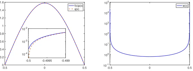
Figure 1: Left: a comparison of the optimal distributionf(x)p(x) and the chosen IS distribution p(x); inset is the zoom-in plot around the tail −0.5 on a logarithmic scale. Right: the weight function.

withϕ(x) and Φ(x) being the probability density function and the cumula-tive distribution function of the standard normal distribution respeccumula-tively. The optimal distribution is f(x)p(x)/I =f(x)p(x) as we note thatI = 1 in this example. We choose the IS distribution to beq(x) =Q5

j=1Nmul(xj,2).

In Figure 1 (left), we plot the IS distribution q(x) and the optimal distri-bution f(x)p(x) for the first dimension (all the dimensions are the same). In Fig. 1 (a) we can see that the IS distribution q and f agree quite well in their main lobes; however, the sampling density q tends to zero moving away from the mean, while by design the function f(x) bounded below by a positive constant 10−3_{. It can be verified that the variance if the IS}

estimator is unbounded, i.e.,V ar( ˆIq) = +∞, and thus the problem poses a

challenge to standard IS simulation.

We estimateE[f] with three different methods: standard IS, DIS, and the

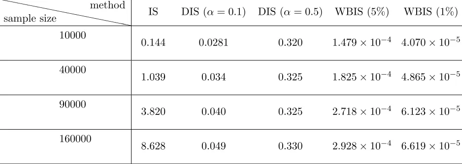
proposed WBIS, all with the chosen IS distribution q. In the DIS method, we use two different values of α: α = 0.1, α = 0.5; in the WBIS method, we use two different significant levels: 5% and 1%. For each methods we compute the estimates ofI with 4 different sample size: 104, 4×104, 9×104 and 16×104 and for each sample size, we repeat the simulation for 105 times. To characterize the performance of each method, we compute the normalized mean square error (NMSE),

N M SE= N

K

K

X

k=1

( ˆIk−I)2, (5.2)

performed andN is the sample size used in each simulation. We summarize the simulation results in Table 1. Also shown in Table 1 is the values of

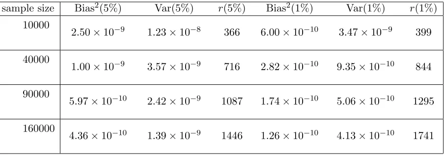
r computed by our method. As we can see from the table, the NMSE of the standard IS increases with respect to sample size, and this is actually unsurprised as the variance of IS is infinity. On the other hand, the NMSE of the DIS is well bounded and does not vary much with respect to the sample size, which indicates that the DIS estimator has a finite variance. However, one can see here that the NMSE of DIS with α= 0.5 is about 10 times of that withα = 0.1, suggesting that the performance of the method is very sensitive to the choice ofα. The table shows that, just like the DIS method, the NMSE of the proposed WBIS method remains about the same level as the sample size increases, and more importantly the NMSE values of WBIS results are much smaller than that of the DIS method with both significance levels, demonstrating a substantially better performance than DIS. To further analyze the WBIS estimator, we list the bias (squared) and the variance in Table 2 for significance levels 1% and 5%. We can see that, in all the results, the bias in the estimator is smaller than the variance of it.

``<sub>``</sub>

``<sub>``</sub>

``<sub>``</sub>

``

sample size

method

IS DIS (α= 0.1) DIS (α= 0.5) WBIS (5%) WBIS (1%)

10000

0.144 0.0281 0.320 1.479×10−4 4.070×10−5

40000

1.039 0.034 0.325 1.825×10−4 4.865×10−5

90000

3.820 0.040 0.325 2.718×10−4 6.123×10−5

160000

8.628 0.049 0.330 2.928×10−4 6.619×10−5

Table 1: The NMSE of the three methods with different sample sizes.

5.2 Portfolio Credit Risk Problem

sample size Bias2(5%) Var(5%) r(5%) Bias2(1%) Var(1%) r(1%)

10000

2.50×10−9 1.23×10−8 366 6.00×10−10 3.47×10−9 399

40000

1.00×10−9 3.57×10−9 716 2.82×10−10 9.35×10−10 844

90000

5.97×10−10 _2.42×10−9 _{1087 1.74×10}−10 _5.06×10−10 ₁₂₉₅

160000

4.36×10−10 1.39×10−9 1446 1.26×10−10 4.13×10−10 1741

Table 2: The bias (squared), the variance, and the thresholdr in the WBIS estimators.

consider a financial institute withmobligors and assess the risk of excessive losses. The settings of the problem are shown below:

• Yk: default indicator for k-th obligor; Yk = 1 if the k-th obligor

de-faults,Yk= 0 otherwise;

• pk: the probability that thek-th obligor defaults;

• ck: the loss resulting from the default of the k-th obligor;

• L=c1Y1+...+cmYm: the total loss from all obligors.

We take the individual default probabilities pk and the lossck as constants

for simplicity, and the goal is to estimate the default probabilityP =P(L > x) for a prescribed loss threshed x. Next we shall describe how the default of an obligor is defined. We characterize the default indicator Yk by the

vector(X1, ..., Xm) of latent variables. SpecificallyYk is given by,

Yk=III{Xk>xk}, k= 1, ..., m

withxkchosen to match the marginal default probabilitypk. Moreover, the

latent variablesXk are assumed to have the form of

Xk=ak1Z1+...+akdZd+bkk, k= 1, ...m,

in which

• Z1, ...Zdare systematic risk factors, each having an independent

• k is an idiosyncratic risk associated with the k-th obligor, each

fol-lowing an independent standard normal distribution;

• ak1, ...akdare the factor loadings for thek-th obligor,a2k1+...+a2kd ≤1;

• bk=

q

1−(a2

k1+...+a2kd).

In the example, the portfolio has 10 systematic risk factors, and there are

m= 1000 obligors in the market. The other settings are

pk= 0.01(1 + sin(16πk/m)), k= 1, ..., m;

ck = (d5k/me)2, k= 1, ..., m.

Firstly, we generate the a group of parameters ak1, ..., akd and bk for k =

1, ..., mfrom a unit ball satisfy (a2_k1+...+a2_kd) +b2_k = 1 . We then choose the threshold loss value to bex= 9500, and by a direct MC simulation with 109 _{samples, we estimate that the default probability is 3.5×10}−6_{, which}

is regarded as the actual value of the default probability. We assume the IS distribution of Gaussian with its mean and covariance determined by using the cross-entropy method [2, 11]. In the cross-entropy method, we use diagonal covariance matrix; moreover, as the specific mean and covariance estimates are highly problem dependent, we choose to omit them here. We use IS, DIS and WBIS to estimate the default probabilityP. We emphasize here that, direct use of the IS method may potentially result in an unbounded variance, while DIS and WBIS can provide a ”safe” estimation of the sought probability.

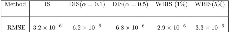
Specifically, for the DIS method we use α = 0.1 and α = 0.5, and for our WBIS method we use the same two significance levels as is in the first example: 1% and 5%. To obtain a reliable comparison, with each method we estimateP using 104 samples and repeat the simulations 2000 times. We then can compute the root mean square error (RMSE) of the 2000 estimates for either method:

RMSE =

v u u t

1

M

M

X

i=1

(Pi−P)2, (5.3)

whereP is the exact value of the sought probability,Pi is the i-th estimate

ofP, andM is the total number of estimates, which in this example is 2000. We summarize the RMSE results in Table 3.

Method IS DIS(α= 0.1) DIS(α= 0.5) WBIS (1%) WBIS(5%)

RMSE 3.2×10−6 6.2×10−6 6.8×10−6 2.9×10−6 3.3×10−6

Table 3: The RMSE of the three methods with different parameter values.

WBIS method is not sensitive to the choice of the significance level, and in practice it is reasonable to use either 1% or 5%. It should be noted here that the IS method also achieves rather good accuracy, suggesting that in this example, the chosen IS distribution actually performs well, and in this case, the proposed WBIS method produces comparable results, while DIS significantly increases the variance.

6

Conclusions

In this paper, we consider the problems where standard IS simulation may have the risk of unbounded variance and we propose a weight bounded IS method to address the issue. The method assumes that the IS distribution is appropriate in the region that has dominant contribution to the integral, i.e., the safe region, and the method performs a standard IS in this safe region and use the resulting estimate as an approximation to the original integral. We then propose a normality test based method to identify the safe region from samples. With numerical examples we demonstrate that the proposed method can result in bounded estimator variance when standard IS fails, and more importantly it can yield more accurate estimates than the often used defensive IS method. In summary, we believe that the proposed WBIS method can be useful in a large class of problems where standard IS simulation may become problematic (i.e., resulting in unbounded variance). We plan to investigate the application of the WBIS method to some real world problems of this type in the future.

Acknowledgements

References

[1] Theodore W Anderson and Donald A Darling. Asymptotic theory of certain” goodness of fit” criteria based on stochastic processes. The annals of mathematical statistics, pages 193–212, 1952.

[2] P.-T. de Boer, D.P. Kroese, S. Mannor, and R.Y. Rubinstein. A tutorial on cross-entropy method. Ann. Oper. Res., 134:19–67, 2005.

[3] Paul Glasserman. Monte Carlo methods in financial engineering, vol-ume 53. Springer Science & Business Media, 2013.

[4] Paul Glasserman and Jingyi Li. Importance sampling for portfolio credit risk. Management science, 51(11):1643–1656, 2005.

[5] Paul Glasserman, Yashan Wang, et al. Counterexamples in importance sampling for large deviations probabilities.The Annals of Applied Prob-ability, 7(3):731–746, 1997.

[6] Tim Hesterberg. Weighted average importance sampling and defensive mixture distributions. Technometrics, 37(2):185–194, 1995.

[7] David P Landau and Kurt Binder.A guide to Monte Carlo simulations in statistical physics. Cambridge university press, 2014.

[8] Jun S Liu. Monte Carlo strategies in scientific computing. Springer Science & Business Media, 2008.

[9] Art Owen and Yi Zhou. Safe and effective importance sampling.Journal of the American Statistical Association, 95(449):135–143, 2000.

[10] Christian Robert and George Casella. Monte Carlo statistical methods. Springer Science & Business Media, 2013.

[11] R.Y. Rubinstein and D.P. Kroese. The cross-entropy method. Springer Science+Business Media, Inc., New York, NY, 2004.