Parity Objectives in Countable MDPs
Stefan Kiefer
∗, Richard Mayr
†, Mahsa Shirmohammadi
∗, Dominik Wojtczak
‡∗University of Oxford, UK †University of Edinburgh, UK
‡University of Liverpool, UK
Abstract—We study countably infinite MDPs with parity ob-jectives, and special cases with a bounded number of colors in the Mostowski hierarchy (including reachability, safety, B ¨uchi and co-B ¨uchi).
In finite MDPs there always exist optimal memoryless deter-ministic (MD) strategies for parity objectives, but this does not generally hold for countably infinite MDPs. In particular, optimal strategies need not exist.
For countable infinite MDPs, we provide a complete picture of the memory requirements of optimal (resp.,-optimal) strategies for all objectives in the Mostowski hierarchy.
In particular, there is a strong dichotomy between two different types of objectives. For the first type, optimal strategies, if they exist, can be chosen MD, while for the second type optimal strategies require infinite memory. (I.e., for all objectives in the Mostowski hierarchy, if finite-memory randomized strategies suffice then also MD-strategies suffice.) Similarly, some objectives admit-optimal MD-strategies, while for others-optimal strate-gies require infinite memory. Such a dichotomy also holds for the subclass of countably infinite MDPs that are finitely branching, though more objectives admit MD-strategies here.
Index Terms—countable MDPs, parity objectives, strategies, memory requirement
I. INTRODUCTION
Markov decision processes (MDPs) are a standard model for dynamic systems that exhibit both stochastic and controlled behavior [23]. The system starts in the initial state and makes a sequence of transitions between states. Depending on the type of the current state, either the controller gets to choose an enabled transition (or a distribution over transitions), or the next transition is chosen randomly according to a defined distribution. By fixing a strategy for the controller, one obtains a probability space of plays of the MDP. The goal of the controller is to optimize the expected value of some objective function on the plays of the MDP. The fundamental ques-tions are “what is the optimal value that the controller can achieve?”, “does there exist an optimal strategy, or only -optimal approximations?”, and “which types of strategies are optimal or -optimal?”.
Such questions have been studied extensively for finite MDPs (see e.g. [9] for a survey) and also for certain types of countably infinite MDPs [23], [21]. However, the literature on countable MDPs is mainly focused on objective functions defined w.r.t. numeric costs (or rewards) that are assigned to transitions, e.g. (discounted) expected total reward or limit-average reward. In contrast, we study qualitative objectives that are expressed by Parity conditions and which are motived by formal verification questions.
There are works that studied particular classes of count-ably infinite, but finitely branching, MDPs that arise from models in automata theory [13], [2], [7], [5], [1]. In each of these papers, a crucial part of the analysis is establishing the existence of optimal strategies of particular structure and memory requirements, but none of them looked at proving such properties for general countable MDPs. Countable MDPs also naturally occur in the analysis of queueing systems [17], gambling [3], and branching processes [22], which have multiple applications. They also show up in the analysis of finite-state models, e.g. in two-player stochastic games [24], [12] when reasoning about an optimal strategy against a fixed (randomised and memory-full) strategy of the opponent.
Finite MDPs vs. Infinite MDPs:It should be noted that many standard properties (and proof techniques) of finite MDPs do not carry over to infinite MDPs.
E.g., given some objective, consider the set of all states in an MDP that have nonzero value. If the MDP is finite then this set is finite and thus there exists some minimal nonzero value. This property does not carry over to infinite MDPs. Here the set of states is infinite and the infimum over the nonzero values can be zero. As a consequence, even for a reachability objective, it is possible that all states have value
>0, but still the value of some states is<1. Such phenomena appear already in infinite-state Markov chains like the classic Gambler’s ruin problem with unfair coin tosses in the player’s favor (0.6 win, 0.4 lose). The value, i.e., the probability of ruin, is always>0, but still<1in every state except the ruin state itself; cf. [14] (Chapt. 14). Another difference is that optimal strategies need not exist, even for qualitative objectives like reachability or parity. Even if some state has value 1, there might not be any single strategy that attains the value 1, but only an infinite family of-optimal strategies for every >0.
Parity objectives:We study general countably infinite MDPs with parity objectives. Parity conditions are widely used in temporal logic and formal verification, e.g., they can express
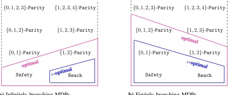
Safety Reach {0,1}-Parity {1,2}-Parity {0,1,2}-Parity {1,2,3}-Parity {0,1,2,3}-Parity {1,2,3,4}-Parity
-optimal optimal
a)Infinitely branching MDPs
Safety Reach
{0,1}-Parity {1,2}-Parity {0,1,2}-Parity {1,2,3}-Parity {0,1,2,3}-Parity {1,2,3,4}-Parity
-optimal optimal
[image:2.612.115.502.50.212.2]b) Finitely branching MDPs
Fig. 1: For countable MDPs, these diagrams show the memory requirements of optimal and-optimal strategies for objectives in the Mostowski hierarchy. An objective in a level of the hierarchy subsumes all objectives in lower levels, e.g.,{0,1,2}-Parity subsumes {1,2}-Parity. We have extended the Mostowski hierarchy to include reachability and safety. The magenta (resp., blue) regions enclose objectives where memoryless deterministic (MD) strategies are sufficient for optimal (resp., -optimal) strategies; for objectives outside the regions, infinite-memory strategies are necessary. The left diagram is for infinitely branching MDPs; e.g.,-optimal strategies for all but reachability objectives require infinite memory, whereas MD-strategies are sufficient for reachability. The right diagram is for finitely branching MDPs; e.g., optimal strategies (if they exist) can be chosen MD for all objectives subsumed by {0,1,2}-Parity.
encoded by numeric transition rewards as in [23], though both types subsume the simpler reachability and safety objectives. There are different types of strategies, depending on whether one can take the whole history of the play into account (history-dependent; (H)), or whether one is limited to a finite amount of memory (finite memory; (F)) or whether deci-sions are based only on the current state (memoryless; (M)). Moreover, the strategy type depends on whether the controller can randomize (R) or is limited to deterministic choices (D). The simplest type MD refers to memoryless deterministic strategies.
The type of strategy needed for an optimal (resp.-optimal) strategy for some objective is also called the strategy com-plexity of the objective. For finite MDPs, MD-strategies are sufficient for all types of qualitative and quantitative parity objectives [8], [10], but the picture is more complex for countably infinite MDPs.
Since optimal strategies need not exist in general, we consider both the strategy complexity of -optimal strategies, and the strategy complexity of optimal strategies under the assumption that they exist. E.g., if an optimal strategy exists, can it be chosen MD?
We provide a complete picture of the memory requirements for objectives in the Mostowski hierarchy, which is summa-rized in Figure 1.
In particular, our results show that there is a strong di-chotomy between two different classes of objectives. For ob-jectives of the first class, optimal strategies, where they exist, can be chosen MD. For objectives of the second class, optimal strategies require infinite memory in general, in the sense that all FR-strategies achieve the objective only with probability
zero. A similar dichotomy applies to-optimal strategies. For certain objectives, -optimal MD-strategies exist, while for all others even -optimal strategies require infinite memory in general. This is a strong dichotomy because there are no objectives in the Mostowski hierarchy for which other types of strategies (MR, FD, or FR) are both necessary and sufficient. Put differently, for all objectives in the Mostowski hierarchy, if FR-strategies suffice then MD-strategies suffice as well.
We also consider the subclass of countable MDPs that are finitely branching. (Note that these generally still have an infinite number of states.) The above mentioned dichotomies apply here as well, though the classes of objectives where optimal (resp. -optimal) strategies can be chosen MD are larger than for general countable MDPs.
objectives in the following sections. In Section V we show that optimal strategies for B¨uchi objectives, where they exist, can be chosen MD, even for infinitely branching MDPs. In Section VI we consider finitely branching MDPs. We show that optimal strategies for{0,1,2}-Parity, where they exist, can be chosen MD (Theorem 16). This is a very general result. E.g., this question had been open (and is non-trivial) even for almost-sure co-B¨uchi objectives. Moreover, we show that -optimal strategies for co-B¨uchi objectives can be chosen MD (Theorem 19). We conclude the paper with a discussion of how some results change when one considers uncountable MDPs. Missing proofs can be found in the full version of this paper [16].
II. PRELIMINARIES
Aprobability distributionover a countable (not necessarily finite) set S is a function f :S →[0,1]s.t. P
s∈Sf(s) = 1.
We use supp(f) ={s∈S|f(s)>0}to denote thesupport off. LetD(S)be the set of all probability distributions overS. We consider countably infinite Markov decision processes (MDPs) M= (S, S2, S,−→, P)where the countable setS of states is partitioned into the setS2 of states of the player and random states S. The relation −→ ⊆ S ×S is the transition relation. We write s−→s0 if (s, s0) ∈ −→, and we assume that each state s has a successor state s0 with
s−→s0. The probability functionP :S → D(S) assigns to each random state s∈S a probability distribution over its successor states. A setT ⊆S is asinkinMif for alls∈T
all successors of s are in T. The MDP M is called finitely branching if each state has only finitely many successors; otherwise, it is infinitely branching. A Markov chain is an MDP where S2=∅, i.e., all states are random states.
We describe the behavior of an MDP as a one-player stochastic game played for infinitely many rounds. The game starts in a given initial state s0. In each round, if the game is in state s ∈ S2 then the player (or controller) chooses a successor state s0 with s−→s0; otherwise the game is in a random state s ∈ S and proceeds randomly to s0 with probabilityP(s)(s0).
Strategies.Aplaywis an infinite sequences0s1· · · of states such that si−→si+1 for all i ≥ 0; let w(i) = si denote the i-th state along w. Apartial play is a finite prefix of a play. We say that (partial) play w visitss if s=w(i) for somei, and that w starts in s if s =w(0). A strategy is a function
σ : S∗S
2 → D(S) that assigns to partial plays ws∈ S∗S
2
a distribution over the successors {s0 ∈ S | s−→s0}. The set of all strategies in M is denoted by ΣM (we omit the subscript and writeΣifMis clear). A (partial) plays0s1· · · is induced by strategy σ if si+1 ∈ supp(σ(s0s1· · ·si)) for
all i with si ∈ S2, and si+1 ∈ supp(P(si)) for all i with si ∈S.
Since this paper focuses on the memory requirements of strategies, we present an equivalent formulation of strategies, emphasizing the amount of memory required to implement a strategy. Strategies can be implemented by probabilistic
transducers T = (M,m0, πu, πs) where M is a countable
set (the memory of the strategy), m0 ∈ M is the initial memory mode and S is the input and output alphabet. The probabilistic transition functionπu:M×S→ D(M)updates
the memory mode of transducer. The probabilistic successor function πs : M×S2 → D(S) outputs the next successor,
wheres0 ∈supp(πs(m, s))implies s−→s0. We extend πu to
D(M)×S → D(M)and πs to D(M)×S2 → D(S), in the
natural way. Moreover, we extendπu to paths byπu(m, ε) =
m and πu(m, s0· · ·sn) = πu(πu(s0· · ·sn−1,m), sn). The
strategy σT : S∗S2 → D(S)induced by the transducer T is
given by σT(s0· · ·sn) := πs(sn, πu(s0· · ·sn−1,m0)). Note that such strategies allow for randomized memory updates and probabilistic successor functions.
Strategies are in generalhistory dependent(H) and random-ized (R). An H-strategyσis finite memory(F) if there exists some transducer T with memory M such that σT = σ and
|M|<∞; otherwise we sayσrequires infinite memory. An F-strategy ismemoryless(M) (also calledpositional) if|M|= 1. We may view M-strategies as functions σ : S2 → D(S). An R-strategy σ is deterministic (D) if πu and πs map to
Dirac distributions; it implies thatσ(w)is a Dirac distribution for all partial plays w. All combinations of the properties in {M,F,H} × {D,R} are possible, e.g., MD stands for memoryless deterministic. HR strategies are the most general type.
Probability Measures. An MDP M= (S, S2, S,−→, P), an initial state s0, and a strategy σ induce a standard probability measure on sets of infinite plays. We write PM,s0,σ(R) for the probability of a measurable set R ⊆
s0Sω of plays starting from s0. It is defined, as usual, by first defining it on the cylinders s0s1. . . snSω, where s1, . . . , sn ∈ S: if s0s1. . . sn is not a partial play induced
by σ then set PM,s0,σ(s0s1. . . snS
ω) = 0; otherwise set
PM,s0,σ(s0s1. . . snS
ω) = Qn−1
i=0 σ(s¯ 0s1. . . si)(si+1), where
¯
σ is the map that extends σ by σ(ws) =¯ P(s) for any
ws∈S∗S. Using Carath´eodory’s extension theorem [4], this defines a unique probability measure PM,s0,σ on measurable subsets ofs0Sω.
Objectives. Let M = (S, S2, S,−→, P) be an MDP. The objective of the player is determined by a predicate on infinite plays. We assume familiarity with the syntax and semantics of the temporal logic LTL [11]. Formulas are interpreted on the structure (S,−→). We use JϕKs⊆sSω to denote the set
of plays starting fromsthat satisfy the LTL formula ϕ. This set is measurable [25], and we just write PM,s,σ(ϕ)instead
of PM,s,σ(JϕK
s). We also write JϕK for
S
s∈SJϕK s.
Given a target set T ⊆ S, the reachability objective is defined byReach(T) = JFTK, i.e., s0s1· · · ∈Reach(T) ⇔
∃i. si ∈ T. The safety objectiveis defined by Safety(T) =
JG¬TK, i.e., s0s1· · · ∈ Safety(T) ⇔ ∀i. si 6∈T. Given a reachability or a safety objective, we can assume without loss of generality thatT is a sink inM.
LetC ⊆Nbe a finite set of colors. Acolor functionCol:
∈ {<,≤,=,≥, >} andQ⊆S, let [Q]Coln :={s∈Q| Col(s)n} be the set of states in Q with color n. The parity objective is defined by
Parity(Col) :=r_ i∈C
GF[S]Col=2·i∧FG[S]Col≤2·iz
,
i.e., Parity(Col) is the set of infinite plays such that the largest color that occurs infinitely often along the play is even. The Mostowski hierarchy [20] classifies parity objectives by restricting the range of the functionColto a set of colorsC ⊆
N. We writeC-Parityfor such restricted parity objectives. In particular, B¨uchi objectives correspond to{1,2}-Parity, and co-B¨uchi objectives correspond to {0,1}-Parity. The objec-tives{0,1,2}-Parityand{1,2,3}-Parityare incomparable, but they both subsume (modulo renaming of colors) B¨uchi and co-B¨uchi objectives. Moreover, both {0,1}-Parity and {1,2}-Parity subsume the reachability objective Reach(T)
(for MDPs with a sink T), by defining the color function so thatCol(s) = 1 ⇔ s6∈T. Similarly, both{0,1}-Parityand {1,2}-Parity subsume Safety(T), by defining Col(s) = 1 ⇔ s∈T.
Optimal and -Optimal Strategies. Given an objective ϕ, the value of state sin an MDP M, denoted by valM(s), is the supremum probability of achieving ϕ, i.e., valM(s) :=
supσ∈ΣPM,s,σ(ϕ). For≥0ands∈S, we say that a
strat-egyσis-optimaliffPM,s,σ(ϕ)≥valM(s)−. A0-optimal strategy is calledoptimal. An optimal strategy isalmost-surely winningifvalM(s) = 1. Unlike in finite-state MDPs, optimal strategies need not exist in countable MDPs, not even for reachability objectives in finitely branching MDPs. However, by the definition of the value, for all > 0, an -optimal strategy exists.
For an objectiveϕand∈ {≥, >}andc∈[0,1], we define
ϕc as the set of statessfor which there exists a strategyσ
withPM,s,σ(ϕ)c. We call a states almost-surely winning
ifs∈
ϕ≥1
, and we callslimit-surely winningifs∈
ϕ≥c
for every constant c < 1 (which is iff valM(s) = 1). On infinite arenas, limit-surely winning states are not necessarily almost-surely winning.
III. OBJECTIVES THAT REQUIRE INFINITE MEMORY
In this section we consider those objectives in the Mostowski hierarchy where optimal (resp., -optimal) strate-gies require infinite memory. In each such case we construct an MDP that witnesses this requirement. In these MDPs, all FR-strategies achieve the objective only with probability 0, while some HD-strategy achieves the objective almost-surely (resp., with arbitrarily high probability).
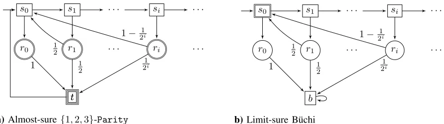
Theorem 1. Letϕ={1,2,3}-Parity. There exists a finitely branching MDPMwith initial state s0 such that
• for all FR-strategies σ, we havePM,s0,σ(ϕ) = 0, • there exists an HD-strategyσsuch thatPM,s0,σ(ϕ) = 1. Hence, optimal (and even almost-surely winning) and -optimal strategies require infinite memory for {1,2,3}-Parity, even in finitely branching MDPs.
The MDP in Theorem 1 is depicted in Figure 2 (left), where Col(si) = 1 and Col(ri) = 2 for all i ∈ N, and Col(t) = 3. For every FR-strategy there is a uniform lower bound on the probability of visiting t between consecutive visits tos0. Hence, unless the strategy with positive probability eventually always stays in states si (and thus also loses the
almost-sure parity objective), in the long-run, the probability of visiting t (with color three) tends to 1, and the parity condition is satisfied with probability 0. Although the player cannot win by any FR-strategy, we construct an HD-strategy
σ such thatPM,s0,σ(ϕ) = 1. This strategy is such that upon the ith visit tos
0, the ladder s0s1· · ·si is traversed and the
transitionsi−→ri is chosen. Moving further along the ladder s0s1s2· · · decreases the probability of visitingtbetween the previous and successive visits tos0. Hence, the probability of visiting color three infinitely often is0.
Remark 1. A strict subclass of finitely branching MDPs are
1-counter MDPs, where a finite-state MDP is augmented with an integer counter [5]. The MDP in Theorem 1 (plus some auxiliary states) is implementable by a1-counter MDP.
Remark 2. The classical Rabin and Streett conditions can encode {1,2,3}-Parity. Thus, optimal and -optimal strate-gies for Rabin/Streett require infinite memory, even in finitely branching countable MDPs.
On finite MDPs, optimal strategies can be chosen MD for parity and Rabin objectives, but not for Streett objectives. Optimal strategies for Streett objectives can be chosen MR or FD [8].
Proof. For an infinite playπ∞, letInf(π∞)be the set of states that π∞ visits infinitely often. Let us recall the Rabin and Streett conditions.
Given a Rabin condition{(E1, F1),(E2, F2),· · ·,(En, Fn)}
withnpairs (orn disjunctions), an infinite playπ∞ satisfies the Rabin condition if there exists a pair (Ei, Fi) such that
Inf(π∞)∩Ei=∅andInf(π∞)∩Fi6=∅. The Rabin condition
{([S]Col=3,[S]Col=2)}
encodes{1,2,3}-Parity, since all satisfying runs must visit states with color2infinitely often and states with color3only finitely often. Note that{1,2,3}-Parityis encoded in a Rabin condition with only one disjunction.
Given a Streett condition{(E1, F1),(E2, F2),· · ·,(En, Fn)}
with n pairs (or n conjunctions), an infinite play π∞
satisfies the Streett condition if Inf(π∞)∩Ei = ∅ implies
Inf(π∞)∩Fi=∅ for all pairs(Ei, Fi). The Streett condition
{([S]Col=2, S),(∅,[S]Col=3)}
encodes{1,2,3}-Parity, since all satisfying runs must visit states with color2infinitely often and states with color3only finitely often.
s0 s1 · · · si · · ·
r0 r1 · · · ri · · ·
tt
1 1
2
1 2i
1 2
1− 1 2i
a) Almost-sure{1,2,3}-Parity
s0 s1 · · · si · · ·
r0 r1 · · · ri · · ·
b
1 1
2
1 2i
1 2
1− 1 2i
[image:5.612.100.547.47.172.2]b)Limit-sure B¨uchi
Fig. 2: Two finitely branching MDPs where the states s∈S2 of the player are drawn as squares and random states s∈S as circles. The color Col(s) of s is indicated with the number of boundaries; for example, a double boundary for color 2. States0 in the MDP on the left is almost-surely winning for{1,2,3}-Parity, but all almost-surely winning strategies require infinite memory. The MDP on the right is such that, for all c >0, strategies that achieve B¨uchi with probability at least c
require infinite memory.
color 2 toX and color 1 toY. Unlike for {1,2,3}-Parity, optimal strategies for {0,1,2}-Parity (and thus also for a single Streett pair) can be chosen MD in finitely branching MDPs (Theorem 16).
It was known that quantitative B¨uchi objectives require infinite memory [18], [2]. For the sake of completeness, we present an example MDP for Proposition 2 in Figure 2 (right).
Proposition 2 ([18]). Let ϕ = {1,2}-Parity be the B¨uchi objective. There exists a finitely branching MDPMwith initial state s0 such that
• for all FR-strategies σ, we havePM,s0,σ(ϕ) = 0, • for every c∈ [0,1), there exists an HD-strategy σ such
that PM,s0,σ(ϕ)≥c.
Hence,-optimal strategies for B¨uchi objectives require infinite memory.
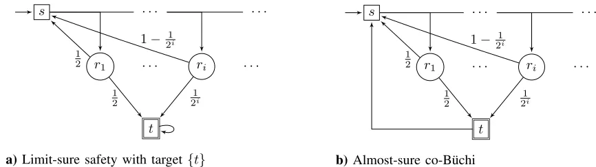
Theorem 3. Let ϕ = Safety(T). There exists an infinitely branching MDPMwith initial state ssuch that
• for all FR-strategies σ, we havePM,s,σ(ϕ) = 0, • for every c∈ [0,1), there exists an HD-strategy σ such
that PM,s,σ(ϕ)≥c.
Hence,-optimal strategies for safety require infinite memory.
The MDP in Theorem 3, depicted in Figure 3 (left), was first introduced in [19]. Since our notion of finite-memory strategies allows for randomized memory updates (in contrast to [19]), our proof is somewhat more general. The target is
T ={t}. For every FR-strategy there is a uniform lower bound on the probability of reaching t between consecutive visits to s0. Since t is absorbing, it will be reached with proba-bility 1. Thus every FR-strategy satisfies the safety objective with probability 0. However, for all n∈N, we construct an HD-strategy σn such thatPM,s,σn(Safety({t}))≥1−
1 2n.
This strategy is such that upon the ith visit to s, the transi-tion s−→ri+n is chosen. Hence, the probability of visiting t
between two successive visits to sdecreases. A more detailed analysis shows that the probability of ever visitingtis bounded by 21n.
Theorem 4. Letϕ={0,1}-Paritybe the co-B¨uchi objective. There exists an infinitely branching MDPMwith initial state
ssuch that
• for all FR-strategiesσ, we have PM,s,σ(ϕ) = 0, • there exists an HD-strategyσsuch thatPM,s,σ(ϕ) = 1.
Hence, optimal (and even almost-surely winning) strategies and-optimal strategies for co-B¨uchi require infinite memory.
The MDP in Theorem 4 is depicted in Figure 3 (right). By a similar argument as in Theorem 3, every FR-strategy achieves co-B¨uchi with probability0. However, the HD-strategyσthat chooses the transition s−→ri upon the ith visit to s is such
that PM,s,σ(ϕ) = 1.
IV. FROM ALMOST-SURE WINNING TO OPTIMAL STRATEGIES
In this section we prove Theorem 5. It says that, for certain objectives, if almost-surely winning strategies (where they exist) can be chosen MD, then optimal strategies (where they exist) can also be chosen MD.
We call a classCof MDPsdownward-closedif every MDP whose transition relation is a subset of the transition relation of some MDP inCis also inC. The class of finitely branching MDPs is downward-closed, and so is the class of MDPs with a fixed sinkT.
We call an objective ϕ prefix-independent in C (where C is a class of MDPs) if for all w1, w2 ∈ S∗ and allw ∈ Sω such that w1w and w2w are infinite plays in an MDP in C we have w1w∈ JϕK ⇐⇒ w2w ∈JϕK. Parity objectives are prefix-independent in the class of all MDPs. Both objectives Reach(T)andSafety(T)are prefix-independent in the class of MDPs with sinkT.
The following theorem provides, under certain conditions, an optimal MD-strategy for all states that have an optimal strategy. In fact, a single MD-strategy is optimal for all states that have an optimal strategy:
s
r1 · · · ri · · ·
t
· · · ·
1 2
1 2i
1 2
1− 1 2i
a) Limit-sure safety with target{t}
s
r1 · · · ri · · ·
t
· · · ·
1 2
1 2i
1 2
1− 1 2i
[image:6.612.92.525.53.175.2]b)Almost-sure co-B¨uchi
Fig. 3: In the infinitely branching MDP on the left, all -optimal strategies for Safety require infinite memory. In the infinitely branching MDP on the right, all optimal (and thus almost-surely winning) strategies for co-B¨uchi require infinite memory.
any M = (S, S2, S,−→, P)∈ C and any s∈ S and any strategyσwithPM,s,σ(ϕ) = 1there exists an MD-strategyσ0
withPM,s,σ0(ϕ) = 1.
Under this condition, for each M ∈ C there is an MD-strategy σ0 such that for alls∈S:
∃σ∈Σ.PM,s,σ(ϕ) =valM(s)
=⇒
PM,s,σ0(ϕ) =valM(s)
The remainder of the section is devoted to the proof of Theorem 5.
For prefix-independent winning conditions, whenever an optimal strategy visits some state, it achieves the value of this state; see Lemma 20 in the full version of the paper [16]. We use this to show that the MDP constructed in the following lemma is well-defined. This MDP,M∗, will be crucial for the proof of Theorem 5. Loosely speaking, M∗ is the MDP M conditioned underϕ.
Lemma 6. Let ϕ be an objective that is prefix-independent in a class C of MDPs. Let M = (S, S2, S,−→, P) ∈ C. Construct an MDPM∗= (S∗, S∗2, S∗,−→∗, P∗)by setting
S∗={s∈S| ∃σ.PM,s,σ(ϕ) =valM(s)>0}
and S∗2 =S∗∩S2 andS∗=S∗∩S and
−→∗={(s, t)∈S∗×S∗|s−→t and ifs∈S∗2
thenvalM(s) =valM(t)}
and P∗:S∗→ D(S∗)so that
P∗(s)(t) =P(s)(t)·
valM(t) valM(s)
for all s∈S∗ andt∈S∗ withs−→∗t. Then:
1) For allσ∈ΣM∗ and alln≥0 and all s0, . . . , sn∈S∗ withs0−→∗s1−→∗ · · · −→∗sn:
PM∗,s0,σ(s0s1· · ·snS
ω) =
PM,s0,σ(s0s1· · ·snS
ω)· valM(sn)
valM(s0)
2) For all s0 ∈ S∗ and all σ ∈ ΣM with PM,s0,σ(ϕ) = valM(s0)>0 and all measurable R ⊆s0Sω we have
PM∗,s0,σ(R) =PM,s0,σ(R|JϕK s0).
The following lemma provides, under certain conditions, a uniform almost-surely winning MD-strategy, i.e., one that works for all initial states at the same time:
Lemma 7. Let M= (S, S2, S,−→, P)be an MDP. Let ϕ be an objective that is prefix-independent in {M}. Suppose that for any s ∈S and any strategy σ with PM,s,σ(ϕ) = 1
there exists an MD-strategy σ0 with PM,s,σ0(ϕ) = 1. Then there is an MD-strategyσ0 such that for all s∈S:
∃σ∈Σ.PM,s,σ(ϕ) = 1
=⇒ PM,s,σ0(ϕ) = 1
Proof. We can assume that all states are almost-surely win-ning, since in order to achieve an almost-sure winning objec-tive, the player must forever remain in almost-surely winning states. So we need to define an MD-strategyσ0 so that for all
s∈S we have PM,s,σ0(ϕ) = 1.
Fix an arbitrary state s1 ∈ S. By assumption there is an MD-strategy σ1 withPM,s1,σ1(ϕ) = 1. Let U1 ⊆ S be the set of states that occur in plays that both start froms1and are induced byσ1. We have PM,s1,σ1(JϕK
s1 ∩Uω
1) = 1. In fact, for anys∈U1and any strategy σthat agrees withσ1 onU1 we have PM,s,σ(JϕK
s∩Uω 1) = 1.
IfU1=S we are done. Otherwise, consider the MDPM1 obtained fromMby fixingσ1onU1(i.e., inM1we can view the states inU1 as random states). We argue that, inM1, for any statesthere is an MD-strategyσ10 withPM1,s,σ10(ϕ) = 1. Indeed, let s ∈ S be any state. Recall that there is an MD-strategy σ with PM,s,σ(ϕ) = 1. Let σ01 be the MD-strategy obtained by restrictingσ to the non-U1 states (recall that the
U1 states are random states in M1). This strategy σ10 almost surely generates a play that either satisfies ϕ without ever enteringU1orat some point entersU1. In the latter case,ϕis satisfied almost surely: this follows from prefix-independence and the fact thatσ01 agrees with σ1 on U1. We conclude that
PM1,s,σ01(ϕ) = 1.
Lets2∈S\U1. We repeat the argument from above, withs2 instead ofs1, and withM1instead ofM. This yields an MD-strategyσ2and a setU23s2withPM1,s2,σ2(JϕK
s2∩Uω 2) = 1. In fact, for anys∈U2 and any strategyσthat agrees withσ2 onU2 and with σ1 on U1 we havePM,s,σ(JϕK
s1, s2, . . . to have Si≥1Ui = S. Define an MD-strategy σ0
such that for any s ∈ S2 we have σ0(s) = σi(s) for the
smallestiwiths∈Ui. Thus, ifs∈Ui, we havePM,s,σ0(ϕ)≥
PM,s,σ0( JϕK
s∩Uω i ) = 1.
The following measure-theoretic lemma will be used to connect probability measures induced by the MDPs M and M∗ from Lemma 6.
Lemma 8. LetS be countable and s∈S. Call a set of the form swSω for w ∈S∗ a cylinder. LetP,P0 be probability measures on sSω defined in the standard way, i.e., first on
cylinders and then extended to all measurable setsR⊆sSω.
Suppose there is x ≥0 such that x· P(C) ≤ P0(C) for all cylindersC. Thenx· P(R)≤ P0(R)holds for all measurable R⊆sSω.
We are ready to prove Theorem 5.
Proof of Theorem 5. As in the statement of the theorem, suppose that ϕ is an objective that is prefix-independent in a downward-closed class C of MDPs so that for any M = (S, S2, S,−→, P) ∈ C and any s ∈ S and any strategyσwithPM,s,σ(ϕ) = 1there exists an MD-strategyσ0
with PM,s,σ0(ϕ) = 1. Let M = (S, S2, S,−→, P) ∈ C. Let M∗ = (S∗, S∗2, S∗,−→∗, P∗)be the MDP defined in Lemma 6. Since Cis downward-closed, we haveM∗∈ C. In particular, ϕis prefix-independent in{M∗}.
First we show that for any s ∈ S∗ there exists an MD-strategy σ0 with PM∗,s,σ0(ϕ) = 1. Indeed, let s ∈ S∗. By the definition of S∗, there is a strategy σ withPM,s,σ(ϕ) =
valM(s) > 0. By Lemma 6.2, we have PM∗,s,σ(ϕ) = 1.
By our assumption on C there exists an MD-strategy σ0 with PM∗,s,σ0(ϕ) = 1.
By Lemma 7, it follows that there is an MD-strategyσ0with PM∗,s,σ0(ϕ) = 1for alls∈S∗. We show that this strategyσ0 satisfies the property claimed in the statement of the theorem. To this end, letn≥0ands0, s1, . . . , sn∈S. Ifs0s1· · ·sn
is a partial play in M∗ then, by Lemma 6.1,
PM∗,s0,σ0(s0s1· · ·snS
ω)
=PM,s0,σ0(s0s1· · ·snS
ω)·valM(sn)
valM(s0)
,
and thus, asvalM(sn)≤1,
valM(s0)· PM∗,s0,σ0(s0s1· · ·snS
ω)
≤ PM,s0,σ0(s0s1· · ·snS
ω).
If s0s1· · ·sn is not a partial play in M∗ then
PM∗,s0,σ0(s0s1· · ·snS
ω) = 0 and the previous inequality
holds as well. Therefore, by Lemma 8, we get for all measurable setsR⊆s0Sω:
valM(s0)· PM∗,s0,σ0(R)≤ PM,s0,σ0(R)
In particular, sincePM∗,s0,σ0(ϕ) = 1, we obtainvalM(s0)≤ PM,s0,σ0(ϕ). The converse inequality PM,s0,σ0(ϕ) ≤ valM(s0) holds by the definition of valM(s0), hence we conclude PM,s0,σ0(ϕ) =valM(s0).
V. WHENMD-STRATEGIES SUFFICE IN GENERAL COUNTABLEMDPS
Ornstein [21] shows that -optimal and optimal strategies for reachability can be chosen MD:
Theorem 9 (from Theorem B in [21]). For every countable MDP M there exist uniform -optimal MD-strategies for reachability objectives ϕ =Reach(T), i.e., for every > 0
there is an MD-strategy σ such that for all s∈ S we have
PM,s,σ(ϕ)≥valM(s)−.
Theorem 10 (follows from Proposition B in [21]). LetM= (S, S2, S,−→, P)be an MDP, andϕ=Reach(T). Lets0∈
S andσbe a strategy withPM,s0,σ(ϕ) = 1. Then there is an MD-strategyσˆ withPM,s0,σˆ(ϕ) = 1.
Both theorems are due to [21]; we give an alternative proof of Theorem 10 in the full version of the paper [16]. We generalize Theorem 10 to B¨uchi objectives, using the principle that B¨uchi is repeated reachability:
Proposition 11. Let M = (S, S2, S,−→, P) be an MDP, and s0 ∈ S, and σ a strategy, and Col : S → {1,2}, and
ϕ= Parity(Col). Suppose PM,s0,σ(ϕ) = 1. Then there is an MD-strategyσ0 withPM,s0,σ0(ϕ) = 1.
By appealing to Theorem 5 it follows:
Theorem 12. Let M be an MDP, Col : S → {1,2}, and ϕ = Parity(Col) be a B¨uchi-objective (subsuming reachability and safety). Then there exists an MD-strategyσ0
that is optimal for all states that have an optimal strategy:
∃σ∈Σ.PM,s,σ(ϕ) =valM(s)=⇒
PM,s,σ0(ϕ) =valM(s)
VI. WHENMD-STRATEGIES SUFFICE IN FINITELY BRANCHINGMDPS
In this section we prove that optimal strategies for {0,1,2}-Parity, where they exist, can be chosen MD (The-orem 16) and that-optimal strategies for co-B¨uchi objectives can be chosen MD (Theorem 19). To prepare the ground for these results, we first consider safety objectives.
A. Optimal MD-strategies for Safety
The following proposition asserts in particular that for safety in finitely branching MDPs, there is no need for merely -optimal strategies, as there always exists an -optimal MD-strategy.
Proposition 13 (from Theorem 7.3.6(a) in [23]). Let M = (S, S2, S,−→, P) be a finitely branching MDP, and T ⊆
S, andϕ=Safety(T). Define an MD-strategy σopt-av (for “optimal avoiding”) that, in each state s, picks a successor state with the largest value valM(s) = supσ∈ΣPM,s,σ(ϕ).
Then for all statess∈Swe havePM,s,σopt-av(ϕ) =valM(s),
i.e.,σopt-av is uniformly optimal.
Definition 1. Let M = (S, S2, S,−→, P) be a finitely branching MDP, Col : S → N a color function, ϕ = Safety([S]Col6=0), σ
opt-av the strategy from Proposition 13 and τ∈[0,1]. We define
SafeM(τ) :={s∈S| PM,s,σopt-av(ϕ)≥τ},
i.e., SafeM(τ)is the set of states from which the player can remain within color-0 states forever with probability ≥τ. We drop the subscript Mwhen the MDPMis understood.
Loosely speaking, the following lemma gives a lower bound on the probability that, starting from a “safe” state, “unsafe” states are forever avoided byσopt-av:
Lemma 14. Let M = (S, S2, S,−→, P) be a finitely branching MDP, Col: S →N a color function and σopt-av the strategy from Proposition 13. Let 0< τ1 ≤τ2 ≤1, and
s∈Safe(τ2). ThenPM,s,σopt-av(GSafe(τ1))≥ τ2−τ1
1−τ1.
Proof. We compute probabilities conditioned under the event GSafe(τ1). Since Safe(τ1) ⊆ [S]Col=0, we have
PM,s,σopt-av(G[S]
Col=0 | GSafe(τ
1)) = 1. From the definition of Safe(τ1) and the Markov property we get
PM,s,σopt-av(G[S]
Col=0| ¬GSafe(τ
1))≤τ1. Applying the law of total probability and writing xfor PM,s,σopt-av(GSafe(τ1))
we obtain:
τ2 ≤ PM,s,σopt-av(G[S]
Col=0) Def. 1
= PM,s,σopt-av(G[S]
Col=0
|GSafe(τ1))·x
+PM,s,σopt-av(G[S]
Col=0| ¬GSafe(τ
1))·(1−x)
≤ x+τ1·(1−x)
It followsx≥ τ2−τ1 1−τ1 .
The following lemma states for all τ < 1 that eventually remaining in color-0 states but outsideSafe(τ)has probability zero.
Lemma 15. Let M = (S, S2, S,−→, P) be a finitely branching MDP, and Col : S → N a color function. Let s be a state, and σ a strategy, and τ < 1. Then PM,s,σ(FG¬Safe(τ)∧FG[S]Col=0) = 0.
B. Optimal MD-strategies for{0,1,2}-Parity
Theorem 16. LetMbe a finitely branching MDP,Col:S→ {0,1,2}, and ϕ= Parity(Col). Then there exists an MD-strategy σ0 that is optimal for all states that have an optimal strategy:
∃σ∈Σ.PM,s,σ(ϕ) =valM(s)=⇒
PM,s,σ0(ϕ) =valM(s)
By appealing to Theorem 5 it suffices to show:
Proposition 17. Let M = (S, S2, S,−→, P) be a finitely branching MDP, ands0∈S, andσa strategy, andCol:S→
{0,1,2}, and ϕ= Parity(Col). Suppose PM,s0,σ(ϕ) = 1. Then there is an MD-strategy σ0 withPM,s0,σ0(ϕ) = 1.
The following simple lemma provides a scheme for proving almost-sure properties.
Lemma 18. Let P be a probability measure over the sample space Ω. Let (Ri)i∈I be a countable partition of Ω in
measurable events. LetE⊆Ωbe a measurable event. Suppose P(Ri∩E) =P(Ri)holds for alli∈I. ThenP(E) = 1.
We are ready to prove Proposition 17.
Proof of Proposition 17. To achieve an almost-sure winning objective, the player must forever remain in states from which the objective can be achieved almost surely. So we can assume without loss of generality that all states are almost-sure winning, i.e., for all s∈S we havePM,s,σ(ϕ) = 1 for
someσ.
We will define an MD-strategyσ0withPM,s,σ0(ϕ) = 1for alls∈S. We first define the MD-strategyσ0 partially for the states inSafeM(13)and then extend the definition ofσ
0 to all
states. For the states inSafeM(13)defineσ 0 :=σ
opt-av as in Proposition 13, see Figure 4. Let M0 be the MDP obtained fromMby restricting the transition relation as prescribed by the partial MD-strategyσ0.
For any τ ∈ [0,1], we have SafeM(τ) = SafeM0(τ). Indeed, since M0 restricts the options of the player, we have SafeM(τ) ⊇ SafeM0(τ). Conversely, let s ∈ SafeM(τ). The strategyσopt-av from Proposition 13 achieves PM,s,σopt-av(G[S]
Col=0) ≥ τ. Since σ
opt-av can be applied in M0, and results in the same Markov chain as applying it in M, we conclude s ∈ SafeM0(τ). This justifies to write Safe(τ)for SafeM(τ) =SafeM0(τ) in the remainder of the proof.
Next we show that, also in M0, for all states s∈S there exists a strategyσ1withPM0,s,σ
1(ϕ) = 1. This strategyσ1 is defined as follows. First play according to a strategyσfrom the statement of the theorem. If and when the play visitsSafe(13), switch to the MD-strategyσopt-av from Proposition 13. If and when the play then visits[S]Col6=0, switch back to a strategyσ
from the statement of the theorem, and so forth.
We show that σ1 achieves PM0,s,σ1(ϕ) = 1. To this end we will use Lemma 18. We partition the runs ofsSωin three
eventsR0,R1,R2 as follows:
• R0 contains the runs whereσ1switches betweenσopt-av andσinfinitely often.
• R1 contains the runs where σ1 eventually only plays according toσopt-av.
• R2 contains the runs where σ1 eventually only plays according toσ.
Each timeσ1switches toσopt-av, there is, by Proposition 13, a probability of at least 13 of never visiting a color-{1,2} state again and thus of never again switching toσ. It follows that PM0,s,σ1(R0) = 0. By the definition of σopt-av we have R1 ⊆JFG[S]
Col=0
K ⊆JϕK, and hence PM0,s,σ1(R1∩ JϕK) =PM0,s,σ1(R1). SincePM,s,σ(ϕ) = 1andϕis prefix-independent, we have PM0,s,σ
1(R2∩JϕK) =PM0,s,σ1(R2). Using Lemma 18, we obtainPM0,s,σ
Safe(13)
Safe(23)
[S]Col=2
σopt-av: avoid[S]Col=1 ˆ
σ: almost-sureReach(Safe(2 3)∪[S]
Col=2)
[image:9.612.160.462.53.184.2]s
Fig. 4: The almost-surely winning MD-strategy σ0 for {0,1,2}-Parity is obtained by combining the MD-strategiesσopt-av andσˆ: playσopt-av insideSafe(13)andσˆ outside that set. A key point is that fixingσopt-av insideSafe(13)does not preventσˆ from achieving its objective.
Next we show that for all s ∈ S the strategy σ1 defined above achievesPM0,s,σ
1(FSafe( 2 3)∨F[S]
Col=2) = 1. To this
end we will use Lemma 18 again. We partition the runs of
sSω into three events R0
1,R02,R00 as follows: • R01=JFG[S]Col=0Ks
• R02=JGF[S]Col=2 K
s
• R00=sSω\JϕKs
We have previously shown that PM0,s,σ
1(ϕ) = 1, hence PM0,s,σ
1(R 0
0) = 0. By Lemma 15, almost all runs inR01 sat-isfy GFSafe(23). SinceJGFSafe(32)K⊆JFSafe(23)K, we have PM0,s,σ
1(R 0
1 ∩JFSafe( 2
3)∨F[S] Col=2
K) = PM0,s,σ1(R 0 1). Since R02 ⊆ JF[S]
Col=2
K, we also have PM0,s,σ1(R 0 2 ∩ JFSafe(
2
3)∨F[S] Col=2
K) =PM0,s,σ1(R 0
2). Using Lemma 18 we obtain PM0,s,σ1(FSafe(2
3)∨F[S]
Col=2) = 1.
Writing T =Safe(23)∪[S]Col=2 we have just shown that for all s ∈ S there is a strategy σ1 with PM0,s,σ
1(FT) =
1. By Lemma 7 there is an MD-strategy σˆ for M0 with
PM0,s,ˆσ(FT) = 1 for all s ∈ S. We extend the (so far partially defined) strategy σ0 by σˆ. Thus we obtain a (fully defined) strategy σ0 for M such that for all s∈ S we have PM,s,σ0(FT) = 1.
It remains to show that for alls∈Swe havePM,s,σ0(ϕ) =
1. To this end we will use Lemma 18 again. We partition the runs of sSω in two eventsR00
1,R002:
• R001=JGFSafe(23)Ks, i.e.,R001 contains the runs that visit Safe(23)infinitely often.
• R002 = JFG¬Safe(23)Ks, i.e., R002 contains the runs that from some point on never visitSafe(23).
Every time a run entersSafe(23), by Lemma 14, the probability is at least 12 that the run remains inSafe(13)forever. It follows that almost all runs in R001 eventually remain in Safe(13)
forever, i.e., PM,s,σ0(R001 ∩
JFGSafe( 1
3)K) = PM,s,σ0(R 00 1). Since Safe(13) ⊆ [S]Col=0, we have
JFGSafe( 1 3)K ⊆ JFG[S]
Col=0
K ⊆ JϕK. Hence also PM,s,σ0(R 00
1 ∩ JϕK) =
PM,s,σ0(R001).
We have previously shown that PM,s,σ0(FT) = 1 holds for all s ∈ S. Hence also PM,s,σ0(GFT) = 1 holds for all
s ∈S. In particular, almost all runs in R002 satisfy GFT. By comparing the definitions ofR002 andT we see that almost all runs in R002 even satisfy GF[S]Col=2. Since
JGF[S] Col=2
K ⊆ JϕK, we obtainPM,s,σ0(R
00
2∩JϕK) =PM,s,σ0(R 00 2).
A final application of Lemma 18 yieldsPM,s,σ0(ϕ) = 1for alls∈S.
C. -Optimal MD-strategies for Co-B¨uchi
Theorem 19. Let M = (S, S2, S,−→, P) be a finitely branching MDP, Col : S → {0,1}, and ϕ= Parity(Col)
be the co-B¨uchi objective. Then there exist uniform-optimal MD-strategies. I.e., for every > 0 there is an MD-strategy
σwithPM,s0,σ(ϕ)≥valM(s0)−for everys0∈S.
Proof. Let 1 >0 be a suitably small number (to be deter-mined later),τ1:= 1−1andSafeM(τ1)defined as in Defi-nition 1. Letσopt-av be the MD-strategy from Proposition 13. FromMwe obtain a modified MDPM0 by fixing all player choices from states in SafeM(τ1)according toσopt-av.
We show thatvalM0(s0)≥valM(s0)−1. By definition of the valuevalM(s0), for everyδ >0there exists a strategy
σδ in M s.t. PM,s0,σδ(ϕ) ≥ valM(s0)−δ. We define a
strategy σδ0 in M0 from state s
0 as follows. First play like
σδ. If and when a state in SafeM(τ1) is reached, play like
σopt-av. This is possible, since no moves from states outside SafeM(τ1)have been fixed inM0, and all moves from states insideSafeM(τ1)have been fixed according toσopt-av. Then we have:
PM0,s 0,σδ0(ϕ)
=PM,s0,σδ(ϕ)
− PM,s0,σδ(FSafeM(τ1))· PM,s0,σδ(ϕ|FSafeM(τ1)) +PM,s0,σδ(FSafeM(τ1))· PM,s0,σ0δ(ϕ|FSafeM(τ1)) ≥ PM,s0,σδ(ϕ)
− PM,s0,σδ(FSafeM(τ1))· PM,s0,σδ(ϕ|FSafeM(τ1)) +PM,s0,σδ(FSafeM(τ1))·τ1
≥valM(s0)−δ− PM,s0,σδ(FSafeM(τ1))(1−τ1)
Since this holds for every δ > 0 we obtain valM0(s0) ≥ valM(s0)−1.
Now let τ2 := 1− 1/k for a suitably large k ≥ 1 (to be determined later) and SafeM0(τ2) be defined as in Definition 1. In particular, SafeM0(τ2) =SafeM(τ2)(by the same argument as in the proof of Proposition 17).
By definition of the value, for every 2 > 0 there exists a strategy σ2 in M
0 with P M0,s
0,σ2(ϕ) ≥ valM0(s0) − 2. Moreover, by Lemma 15 and τ2 <
1, PM0,s
0,σ(FSafeM0(τ2)) ≥ PM0,s0,σ(ϕ) for every strategy σ and thus in particular for σ2. Therefore, PM0,s0,σ
2(FSafeM0(τ2))≥valM0(s0)−2. By Theorem 9, for every 3 >0 there exists an MD-strategyσ0 in M0 with
PM0,s
0,σ0(FSafeM0(τ2))≥valM0(s0)−2−3. In particular,
σ0must coincide withσopt-av at all states inSafeM(τ1), since inM0 these choices are already fixed.
We obtain the MD-strategyσinMby combining the
MD-strategies σ0 andσopt-av. The strategy σ plays like σ0 at all
states outside SafeM(τ1) and like σopt-av at all states inside SafeM(τ1).
In order to show that σ has the required property
PM,s0,σ(ϕ)≥valM(s0)−, we first estimate the probability
that a play according toσwill never leave the setSafeM(τ1) after having visited a state in SafeM0(τ2).
Let s∈SafeM0(τ2). Then, by Lemma 14,
PM,s,σopt-av(GSafe(τ1)) ≥
τ2−τ1
1−τ1
= (1−1/k)−(1−1) 1
= 1−1
k.
In particular we also havePM,s,σ(GSafe(τ1))≥1−
1 k, since σcoincides withσopt-av inside the setSafeM(τ1). Finally we obtain:
PM,s0,σ(ϕ) ≥ PM,s0,σ(FSafeM0(τ2))
· PM,s0,σ(FGSafeM(τ1)|FSafeM0(τ2))
≥ PM0,s
0,σ0(FSafeM0(τ2))·(1−1/k) ≥ (valM0(s0)−2−3)·(1−1/k)
≥ (valM(s0)−1−2−3)·(1−1/k)
This holds for every 1, 2, 3 > 0 and every k ≥ 1, and moreover valM(s0)≤1. Thus we can set 1 =2=3 :=
/6 andk:=2 and obtain PM,s0,σ(ϕ)≥valM(s0)− for
everys0∈S as required.
VII. DISCUSSION
Our results on the memory requirements of ()-optimal strategies (Figure 1) directly imply how much memory is needed to win quantitative objectives of type ϕc (consid-ered, e.g., in [6]). For c < 1 the assumed winning strategy might have to be an -optimal one, since optimal strategies do not always exist. Thus MD-strategies are only sufficient for reachability objectives in countable MDPs (resp., for
{0,1}-Parity, safety and reachability objectives in finitely branching MDPs). In the special case of
ϕ≥1
objectives (i.e., winning almost-surely), the winning strategy (assuming it exists) must be optimal. Thus MD-strategies are only sufficient for safety, reachability and{1,2}-Parityin countable MDPs (resp., for all objectives subsumed by {0,1,2}-Parity in finitely branching MDPs).
In this paper we have studied countable MDPs. Not all our results carry over to uncountable MDPs. The first issue is measurability. The probabilities are only well-defined if the strategies are measurable functions, which might not exist without further conditions on the MDP; cf. Section 2.3 in [23]. Another issue is that strategies cannot generally be chosen uniform, i.e., independent of the initial state. E.g., in countable MDPs -optimal strategies for reachability can be chosen uniform MD (Theorem 9), but this does not carry over to uncountable MDPs (Thm. A in [21]). However, optimal strategies for reachability, if they exist, can be chosen uniform MD (Proposition B in [21]).
Acknowledgements. This work was partially supported by the EPSRC through grants EP/M027287/1, EP/M027651/1, EP/P020909/1 and EP/M003795/1 and by St. John’s College, Oxford.
REFERENCES
[1] P.A. Abdulla, R. Ciobanu, R. Mayr, A. Sangnier, and J. Sproston. Qualitative analysis of VASS-induced MDPs. In Proc. of FOSSACS 2016, volume 9634 ofLNCS, 2016.
[2] C. Baier, N. Bertrand, and Ph. Schnoebelen. Verifying nondeterministic probabilistic channel systems against omega-regular linear-time proper-ties.ACM Transactions on Computational Logic, 9, 2007.
[3] N. Berger, N. Kapur, L. J. Schulman, and V. V. Vazirani. Solvency games. In Ramesh Hariharan, Madhavan Mukund, and V. Vinay, editors, IARCS Annual Conference on Foundations of Software Technology and Theoretical Computer Science, FSTTCS 2008, December 9-11, 2008, Bangalore, India, pages 61–72, 2008.
[4] P. Billingsley. Probability and Measure. Wiley, New York, NY, 1995. Third Edition.
[5] T. Br´azdil, V. Broˇzek, K. Etessami, A. Kuˇcera, and D. Wojtczak. One-counter Markov decision processes. InSODA’10, pages 863–874. SIAM, 2010.
[6] T. Br´azdil, V. Broˇzek, A. Kuˇcera, and J. Obdrz´alek. Qualitative reachability in stochastic BPA games. Information and Computation, 209, 2011.
[7] T. Br´azdil, V. Broˇzek, V. Forejt, and A. Kuˇcera. Reachability in recursive Markov decision processes.Information and Computation, 206(5):520– 537, 2008.
[8] K. Chatterjee, L. de Alfaro, and T. Henzinger. Trading memory for randomness. InProceedings of the First Annual Conference on Quan-titative Evaluation of Systems (QEST), pages 206–217. IEEE Computer Society Press, 2004.
[9] K. Chatterjee and T. Henzinger. A survey of stochasticω-regular games. Journal of Computer and System Sciences, 78(2):394–413, 2012. [10] K. Chatterjee, M. Jurdzi´nski, and T. Henzinger. Quantitative stochastic
parity games. InProceedings of the Fifteenth Annual ACM-SIAM Sympo-sium on Discrete Algorithms, SODA ’04, pages 121–130, Philadelphia, PA, USA, 2004. Society for Industrial and Applied Mathematics. [11] E.M. Clarke, O. Grumberg, and D. Peled.Model Checking. MIT Press,
Dec. 1999.
[12] A. Condon. The complexity of stochastic games. Information and Computation, 96(2):203–224, 1992.
[13] K. Etessami and M. Yannakakis. Recursive Markov decision processes and recursive stochastic games. In ICALP’05, volume 3580 ofLNCS, pages 891–903. Springer, 2005.
[15] E. Gr¨adel, W. Thomas, and T. Wilke, editors. Automata, Logics, and Infinite Games, volume 2500 ofLNCS, 2002.
[16] S. Kiefer, R. Mayr, M. Shirmohammadi, and D. Wojtczak. Parity ob-jectives in countable mdps. Technical report, arxiv.org, 2017. Available athttps://arxiv.org/pdf/1704.04490.pdf.
[17] M.Y. Kitaev and V.V. Rykov. Controlled queueing system. CRC press, 1995.
[18] J. Krˇc´al. Determinacy and Optimal Strategies in Stochastic Games. Master’s thesis, Masaryk University, School of Informatics, Brno, Czech Republic, 2009.
[19] A. Kuˇcera. Turn-based stochastic games. In Krzysztof R. Apt and Erich Gr¨adel, editors,Lectures in Game Theory for Computer Scientists. Cambridge University Press, 2011.
[20] A. Mostowski. Regular expressions for infinite trees and a standard form of automata. InComputation Theory, volume 208 ofLNCS, pages 157–168, 1984.
[21] D. Ornstein. On the existence of stationary optimal strategies. Proc. Am. Math. Soc., 20:563–569, 1969.
[22] S.P. Pliska. Optimization of multitype branching processes.Management Science, 23(2):117–124, 1976.
[23] M. L. Puterman. Markov Decision Processes. Wiley, 1994.
[24] L.S. Shapley. Stochastic games. Proceedings of the national academy of sciences, 39(10):1095–1100, 1953.