Article
Surface Completion using Laplacian Transform
Pongsagon Vichitvejpaisal
aand Pizzanu Kanongchaiyos
bDepartment of Computer Engineering, Faculty of Engineering, Chulalongkorn University, Bangkok 10330, Thailand
E-mail: a[email protected], b[email protected] (Corresponding author)
Abstract. Model acquisition processes usually produce incomplete surfaces due to the technical constrains. This research presents the algorithm to perform surface completion using the available surface’s context. Previous works on surface completions do not handle surfaces with near-regular pattern or irregular patterns well. The main goal of this research is to synthesize surface for hole that will have similar surface’s context or geometric details as the hole’s surrounding. This research uses multi-resolution approach to decompose the model into low-frequency part and high-frequency part. The low-frequency part is filled smoothly. The high-frequency part are transformed it into the Laplacian coordinate and filled using example-based synthesize approach. The algorithm is tested with planar surfaces and curve surfaces with all kind of relief patterns. The results indicate that the holes can be completed with the geometric detail similar to the surrounding surface.
Keywords: Surface completion, multi-resolution decomposition, example-based synthesis,
Laplacian transform.
ENGINEERING JOURNAL Volume 18 Issue 1
1.
Introduction
In recent years, we have seen widely spread use of 3D model acquisition systems. The acquisition process is fast and convenient. Many engineering and scientific simulations which require geometric data will gain great benefits from this development. However, the acquired surface usually incomplete due to many reasons such as noise, limited viewpoints, self-occlusion, and technological constrains. The incompleteness of the surface or holes is needed to be filled before the further use of the acquired model. In order for 3D scanning systems to be widely available to the research communities, robust and easy-to-use surface completion methods need to be developed for the users.
Surfaces can be categorized into smooth surfaces and non-smooth surfaces. Smooth surfaces are surfaces with low geometric variations. There are no geometric details or relief information on the surfaces. On the other hand, non-smooth surfaces exhibits relief patterns on the surfaces. This type of surfaces require much more time in manually completing them than the smooth surfaces, since the users have to craft the relief of the surface to make overall surface looks harmony. Recent researches have investigated non-smooth surface completion [1-4]. However, surfaces with regular or irregular relief patterns are still challenging cases that we want to focus on this work. This research is built on the two ideas, multi-resolution decomposition of meshes and example-based synthesis.
The multi-resolution decomposition [5] views the surface as compose of low-frequency part which represents the overall surface structure and high-frequency part which represents the geometric surface detail. This view, in many ways, reflects the human observation on object shapes. The technique is used extensively in model editing process [6].
This work decomposes the surface into two parts, the coarse mesh, the low-frequency part of the surface, and the relief mesh, the high-frequency part of the surface. First, the hole of the coarse mesh is smoothly filled. Then, the relief pattern is transferred to this hole. This is to ensure that both the structure of the filled hole and the relief pattern on the hole are consistent with the input surfaces.
[image:2.595.101.490.487.671.2]This research adapts the idea of the example-based framework of texture synthesis [7] to transfer the relief pattern to the smoothly filled hole. However, for the mesh domain, some important aspects need to be solved. First, mesh topologies do not align regularly in uniform grid style as in images. Meshes that are similar in shape may differ in topology considerably making the comparison between the two vertices' neighborhoods impossible. Second, a new surface similarity metric or surface signature has to be defined spatially at each point of the surface in order to use with the example-based framework.
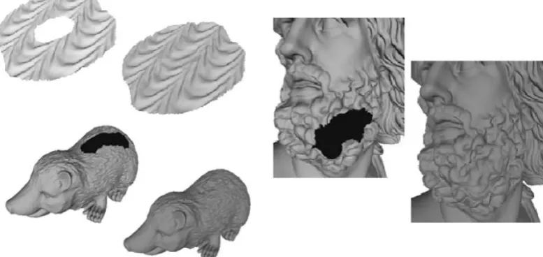
Fig. 1. Context-based surface completion of non-smooth surfaces using our proposed method. The method analyzes the existing relief patterns of the surface in Laplacian domain and transfers them to the smoothly filled hole. The proposed method can handle regular, irregular and stochastic relief.
normal of each point on the surface instead of the position. Figure 1 shows the surface completion result from our proposed method. Note the relief pattern that exhibit on the synthesis surface. The seam between the synthesis surface and the input surface is hardly visible. Note that our method does not need to modify the exiting surface at all.
2.
Related Works on Surface Completion
Surface completion can be broadly divided into two categories: one that does not consider contextual surface information and the other one that fill the hole with the available geometrical detail. Many authors proposed methods to smoothly fill the incomplete surfaces. Notably, Liepa [8] presents a method that can fill the hole smoothly and the filled surface preserved the overall structure of the model. The author use dynamic algorithm to fill the hole with subject to minimizing surface area. Davis et al. [9] use the diffusion process to fill the hole. This method performs voxelization of the model and the cell is classified as inside, outside or on the surface boundary. Other researchers [10-11] solve the problem of surface reconstruction from point clouds by the use of active contour base method. The minimization technique is used to propagate the active contour to fit the given point clouds as much as possible. However, the filled surface is smooth and lack of geometric details. For a large hole, the visual perception can be distracting. They also have to convert the model to volumetric representation which required computational time and memory consumption.
Some authors consider contextual information when perform surface completion. Schnabel et al. [2] use primitives as guidance for surface completion. They first fit the model with the predefined primitives and extended the primitives shape to fill the holes. Their works apply well for CAD model. Pauly et al. [1] perform surface completion using model database. The database has to contain the stock models that similar to the one it try to complete.
Shaft et al. [3] propose an example-base method to do context filling of holes. They fill the missing surface iteratively from coarse to fine level using an octree. They use the signed distance vectors of grid corners as the surface signature for surface similarity test. Park et al. [12] present a method to do surface completion that preserves both shape and appearance. They use grid to divide the surface into patches and do parameterization on each patch. For each patch, the six signatures of average, maximum and minimum of principle curvatures are used to perform shape similarity test. Although they use curvatures as signatures, the six statistic information of curvature can only represent the overall patch curvature but not the geometric context of the surface. In addition, by pasting the whole patch to a hole, the quality on the hole boundary can be noticeably different from other parts of the filling surface even with the use of surface blending. Bendels [13] and Breckon et al. [4] method first fit the whole model with a primitive, such as a plane, sphere or cylinder. Then, the primitive is used as a base surface to sample the vertex displacement vectors from the original surface. The vertex displacement vectors are used as surface signature to search for the similarity. This method may have difficulty with non-height field surfaces which cannot be represented by the vertex displacement vectors and the surface with steep surface detail can produce high distortion result from sampling.
All of the above methods have shown impressive results but do not truly use signatures that can reflect the local properties of the surface. Furthermore, for a large hole, the filled area should also preserve the overall surface structure of the model. The example-based method which fills small patch by patch lacks the knowledge of the higher view of the surface structure. Unfortunately, analyzing relief pattern and transferring it to the hole's surface is not trivial. Usually, most of the previous works on non-smooth surface completion can handle patterns that are stochastic. However, relief patterns that contain near-regular or irnear-regular structures are still a challenging problem.
3.
Background on Laplacian Coordinate
Laplacian operator is defined as the divergence of the gradient and can be written as the sum of second partial derivatives:
2
2
i i
f
f
div f
x
(1)For a given function fdefined on a manifold surface
S
the Laplacian-Beltrami is defined as [18]:S
f
div
S Sf
(2)Applied to the coordinate function X of the surface, the Laplacian-Beltrami operator evaluates to the mean curvature,
H
, multiple by normal, n:Hn
x
S
2
(3)Let V {v1,...,vn}be the set of vertices in absolute Cartesian coordinate, {i} be the set of vertices in
Laplacian coordinate. For discrete Laplacian-Beltrami operator, it can be approximated using Geometric Mesh Laplacian [19].
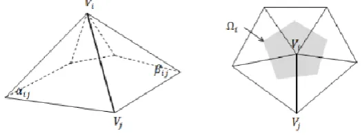
) ( ) )( cot (cot 2 1 1 i N j j i ij ij ii
v v
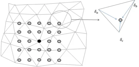
(4)where i is the area of the Voronoi cell constructed around the faces of vertex i (Fig. 2). N(i) are the
neighborhood vertex of i. ij and ij are the two angles that opposite to the edge ij.
We can construct a adjacency matrix L such that LV, that is i L(vi). Matrix L can be viewed as
the adjacency matrix of a graph of mesh. The dimension of the matrix L is nxn, where n is the number of mesh's vertices. The matrix is used to multiply each component (x, y, z) of Cartesian coordinate separately;
) , ,
( iz
y i x i
i
[image:4.595.167.430.426.526.2] .
Fig. 2. The angles and the Voronoi cell (shaded area) used for the Geometric Mesh Laplacian computation.
One property of the Laplacian coordinate is that it is translation invariant. As a result, matrix L has
rank = n-1 therefore we cannot compute its invert matrix. To reconstruct the Cartesian coordinate, we can assign the Cartesian coordinate to a vertex in the matrix to get a full rank system and therefore has the unique solution. The inverse Laplacian transform thus required solving a linear system of equation.
In practical application, such as model editing, we assign the Cartesian coordinate to more than one vertex. These vertices are called anchor vertices. Let C{1,2,...,m} be the set of indices of those vertex that
we assign spatial coordinatevici,iC. This additional constrain makes the linear system over-determine.
However, we can solve for a unique solution in the least-square sense [20]:
2
arg min
(
)
v
V
L V
(5)distributes the error across the domain. This feature is an advantage when perform mesh editing operation because distortion error is unavoidable in many situations.
4.
Proposed Method Laplacian Coordinate
4.1. Overview
This work represents the 3D surfaces with polygon meshes. The input of the algorithm is a mesh with a hole. The mesh should be regular, uniform and composed of isotropic triangles. These criteria are favored since the algorithm is operated on vertices. The fairing method can be applied if the input mesh does not have the specific qualities. If the model contains many holes, each hole is filled independently, one hole at a time.
The overview of the algorithm is shown in Fig. 3. The process of the algorithm is to smoothly fill the hole first and then extract the relief pattern from the surrounding surface and transfer it to the filled hole. The challenges of this work are on how to extract the relief pattern, how to represent it and how to transfer it to the smoothly filled hole.
[image:5.595.134.459.349.576.2]The key idea of the algorithm is to use multi-resolution decomposition to extract the relief pattern and to use Laplacian coordinate to represent it. Laplacian coordinate defines the local geometric properties, which are normal and curvature, of each surface point. The surface signature can be defined for each vertex using the Laplacian coordinate of neighborhood vertices. In this way, this Laplacian signature can be used with the example-based framework to transfer the relief pattern to the smoothly filled surface.
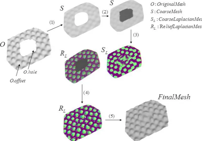
Fig. 3. The high-level algorithm pipeline. First, the surface is smoothed and smoothly filled. Then, the relief pattern is extracted and represented in Laplacian coordinate. The pattern is transferred to the hole area and reconstructed to Cartesian coordinate.
For an input surface O, the offset region around the hole boundary is computed to use as a relief pattern exemplar. The offset region around the hole is used because it is likely to contain the same pattern as the missing surface. However, users are free to choose the exemplar region as appropriate. The exemplar region should cover the relief pattern exhibited on the surface.
Mesh O is divided into two regions: region O.hole which is the region that is needed to be filled and is now empty and region O.offset which is the offset region around the hole boundary (Fig. 3). Other meshes that are constructed further in the algorithm are composed of the hole part and the offset part. The surface part outside the offset region is not use in the surface completion algorithm. Meshes with subscript L are represented in Laplacian coordinate. Those that do not are represented in Cartesian coordinate.
Laplacian coordinate using Geometric Mesh Laplacian which result in mesh OLand mesh SL respectively.
Mesh OL and mesh SL have the same mesh topology as in mesh O and mesh S but instead of storing
vertex position, they store Laplacian coordinate.
The relief mesh, RL, is obtained by subtracting OL with SL (step 3, in Fig. 3). The hole's region of the
relief mesh, RL..hole, is filled using the relief example from the offset region, RL..offset (step 4, in Fig. 3).
Finally, the coarse mesh SL..hole and relief mesh RL..hole are combined to reconstruct the completely filled mesh O.hole (step 5, in Fig. 3). In this way, the filled surface can preserve both the surface structure and surface contextual detail.
4.2. Multi-Resolution Decomposition on Mesh
Usually in mesh decomposition, the coarse mesh is obtained by perform mesh smoothing and the relief mesh is computed using normal displacement method. Normal displacement [21-22] uses the normal of the base surface or coarse surface to sample the original surface in order to get the displacement vectors. The problem of this method is that the surface has to be representable by a height field function. Depend on the geometry of the base mesh, sampling the original mesh can introduce distortion in geometric information. And due to undersampling artifact, the neighbor displacement vectors can have discontinuity even though the original surface is connected.
In this research, Laplacian representation is proposed to use with the multi-resolution decomposition. Laplacian coordinate does not suffer from the sampling problem as in the Normal displacement method and can be used to represent any 2-manifold surfaces. The relief mesh is represented as the difference between the Laplacian coordinate of the original surface and the Laplacian coordinate of the coarse detail surface, RLOLSL.
In representing the relief mesh, RLcannot be used directly as the relief mesh since its Laplacian
coordinate, , is still in the world coordinate. The Laplacian of the relief mesh has to be defined relatively to the coarse mesh. Since, this research views original mesh as compose of relief mesh and coarse mesh. The Laplacian coordinate, , of each vertex of RL has to be transformed to tangent space of the
corresponding vertex of the coarse mesh. For each vertex, the three axis of the tangent space can be defined using the normal vector, the binormal vector and the tangent vector of that vertex.
For a given vertex on the coarse mesh S, let B, N, T be the normal vector, tangent vector and binormal vector of that vertex respectively. The matrix that used to transform Laplacian coordinate from world space to tangent space can be defined as [BT NT TT].
[image:6.595.236.358.564.742.2]Mesh parameterization is needed to compute the binormal vector and the tangent vector (section 4.4). This research uses barycentric map to construct conformal map parameterization. The mapping is then used to consistently define local axis for each vertex points on the coarse mesh. This mapping can also be used with mesh S and mesh R, since both have the same mesh topology as mesh O.
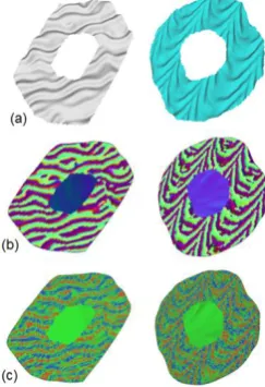
Figure 4(b) shows the normal component of the Laplacian representations. The green color represents the normal vectors that have the same direction as the normal vectors of the coarse mesh, while the blue color represents the normal vectors that have the opposite direction with the normal vectors of the coarse mesh. Figure 4(c) shows the mean curvature component of the Laplacian representations. The blue color indicates the positive curvature. The red color indicates the negative curvature. The green color indicates the zero curvature.
4.3. Coarse Mesh Completion
The coarse mesh S.offset is obtained by performing mesh smoothing. This research uses Curvature flow to do mesh smoothing [23] on O.offset.
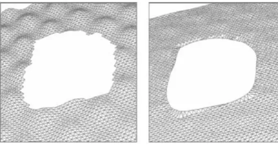
Mesh smoothing may alternates the shape of the hole boundary considerably (Fig .5) . This seems to be problematic at first as the shape of the filled hole is not match the shape of the original hole boundary. However, with the use of Laplacian representation, OL.hole can be reconstructed by choosing the anchor vertices to be the positions of the original hole boundary. The reconstructed OL.hole fuses seamlessly with the O offsetL. . The least-square solver attempts to reconstruct the Cartesian coordinate while preserve the
[image:7.595.166.444.364.509.2]mean curvature normal of each point as much as possible. The geometric distortion that may happen is distributed over the surface and hence unnoticeable. On the other hand, if the hole boundary is fix when performing mesh smoothing, S.hole computed from the coarse mesh completion will not be smooth and it will not reflect the coarse resolution of the original surface. The result will have a downside effect on the relief mesh extraction.
Fig. 5. The hole boundary is rounder due to effect of mesh smoothing.
This research use Liepa's algorithm [8] to perform coarse mesh completion. The algorithm performs hole triangulation, mesh refinement and fairing. Liepa's algorithm is used in coarse mesh completion because it can produce smooth filling surface with minimize surface area and surface dihedral angle.
4.4. Computing Mesh Parameterization
As introduced in section 4.2, mesh parameterization is needed to defined binormal vectors and tangent vectors for computing tangent space of RL. The Laplacian signature that is used with the example-based
framework also requires surface parameterization to consistently define the orientation of each surface point.
This research computes the mapping between squared planar surface and the surface of mesh O. This mapping can also be used with mesh S and mesh R, since both have the same mesh topology as mesh O.
Although there is some distortion in the mapping, this is not going to be an issue, since this research only uses parameterization for defining the binormal direction and the tangent direction for each point on the surface.
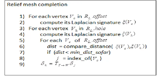
4.5. Relief Mesh Completion
The example-based framework is used to fill the region RL..hole. The region RL..offset is used as the
exemplar. The relief information of RL..hole is still empty since the hole region is only smoothly fill and have no relief information. The Laplacian coordinates of every vertices in RL..hole have value of zero. The relief pattern encoded in Laplacian coordinate from the offset region are used to transferred to RL..hole. The pseudocode is presented in Fig. 6.
[image:8.595.143.466.321.482.2]This research uses pixel-based synthesis [24] approach by transferring the Laplacian coordinate of the hole region to the offset region vertex by vertex. The patch-based synthesis can have an issue with the differences in mesh topology between RL..hole and RL..offset. If the mesh topologies of the two regions are different, Laplacian coordinates cannot be copied directly from one region to the other. In addition, patch-based synthesis can complicate the surface signature definition since the shape and the area of each patch may vary from each other.
Fig. 6. The pseudocode for relief mesh completion.
Let VO be the set of vertices of RL..offset, Vo is an element in VO. Let VH be the set of vertices of RL..hole,
h
V is an element in VH. For each vertex in RL..offset, Vo, its Laplacian signature (Vo) is computed from the
collection of Laplacian coordinates of the sampling points in the neighborhood region of vertex Vo.
The algorithm starts at the vertex on the boundary of RL..hole. It then visits other vertices of VH in
spiral fashion. Basically, the spiral traversal is done using breadth first search algorithm using queue data structure. At the initialize step, the boundary vertices are enqueued to the queue. The last visited vertex is the one located around the center of the hole region.
By visiting vertices in this manner, many neighborhood vertices around VH will already have the Laplacian coordinates assigned and can be used to compute the Laplacian signature for the vertex Vh. If
there are too few neighborhood vertices to use in computing the Laplacian signature, the Laplacian signature may not reflect the characteristic of the relief pattern of a surface patch.
For each vertex in RL..hole, Vh, the algorithm searches for the Vo that have the best matching Laplacian
signature. The Laplacian coordinate of Vo is transferred to Vh. The algorithm terminates when all vertices in
H
V are visited and have received the Laplacian coordinate from VO.
4.5.1. Computing Laplacian signatures
texture. Vertices may not have an equal number of neighborhoods. Vertices may not uniformly distribute on the surface. These are the problems of irregularity of mesh topologies. Furthermore, surface is non-planar like texture.
In this research, for any given vertex, Vi, Laplacian surface signature ( )Vi is defined as the collection of tangent space Laplacian coordinates
1n of the sampling points in the neighborhood region of vertexi V:
n
i
V
( ) 1, 2,..., (6)
where n is the number of sampling point.
[image:9.595.170.442.251.383.2]Laplacian coordinate is used because it can be defined on each point of the surface. It also represents the geometric properties of each point, the curvature and normal, which define the visual characteristic of a surface.
Fig. 7. An example of 5x5 sampling points with 3-nearest neighbors interpolation from vertices that are used to define the Laplacian signature. (The computation is done in uv space.)
The neighborhood region of vertex Vi, N V( )i , is a squared region center at Vi. We use uv space (computed from mesh parameterization) in finding the neighbors, not the Euclidean space. The dimension of this region is discretized so that it is defined by the odd integer values, such as 5x5, 7x7. The dimensional unit is defined to be the inverse of the square root of the number of vertices in the mesh. For example, a mesh with fairly uniform polygons areas, the dimensional unit is approximately equal to the average edge length of a mesh in Euclidean space.
The sampling points are sampled uniformly in grid-based style around a given vertex Vi with the step size equal to the dimensional unit. For example, the 7x7 region has 48 sampling points or 48 components (Vertex Vi is not used as the sampling point). The Laplacian coordinate of each sampling point is interpolated from the Laplacian coordinate of the k-nearest vertices around that sampling point (Fig. 7). The k-nearest vertices are weighted according to the inverse squared distance of the sampling point.
Using Laplacian coordinates from the sampling points instead of vertices can solve the irregularity problem of mesh topologies. The sampling is also done directly on the surface (in uv space), thus there is no sampling artifact as presented in normal displacement sampling. In addition, this method does not need to flatten the mesh in order to find the nearest neighbors.
In the regions around the mesh boundary, some sampling points may not be defined because they are out of bound and will not be included in the signature (Fig. 8). In addition, sampling points around the unvisited Vh are not included in the signature since they do not have the relief information from the offset
Fig. 8. The red sampling points which are in the hole region or outside the offset region are not used to compute for the surface signature. Only the green sampling points are used to compute for the surface signature.
The size of this region can be set by the user and uses for every vertex on the mesh. In practice, the neighborhood size should larger than the geometric feature of the surface, so that it can contain enough information of the relief pattern.
4.5.2. Comparing Laplacian signatures
Two Laplacian signatures are comparable if they have the same number of components. The comparison is done to determine how the two patches are similar visually to each other. Two components from the different signatures with the same index are compared to each other one-to-one. Given two Laplacian signatures (Vi)
ik ;k[1..n] and (Vj)
jk ;k[1..n] where n is the number of sampling points in theneighborhood region. This research defines the distance metric as:
1
1 n
H ik jk
k
Dist H H
n
(7)
2 2 2
1 1 n
x x y y z z
n ik jk ik jk ik jk
k
Dist n n n n n n
n
(8)* (1 ) *
Hn n H
Dist w Dist w Dist (9) where W is the user adjustable weight, Hik is the mean curvature component and nik is the normal
component of the Laplacian coordinate
ik.Finding the best matching ( )Vi for all given (Vj) of the hole region is done in a brute force style thus result in quadratic time complexity. This part can be speed up by using acceleration structure such as k-d tree to store all the signatures of the offset region and then use this tree to compare with the signature from the hole region. This adaptation can result in O(n/log(n)) complexity. However, the comparison may not be done fairly for each component of the signature. The components near the root node would have more influence than the components near the leaf nodes.
4.5.3. Transferring Laplacian coordinates
When transferring the Laplacian coordinate of Vo to Vh, the different in transformed space has to be
[image:10.595.231.392.82.193.2]Fig. 9. The transformation to world space is required when transferring Laplacian coordinate from the offset region to the hole region.
4.6. Combining Coarse Mesh and Relief Mesh
The Laplacian coordinate of mesh RL..hole and SL..hole are combined to obtain OL..hole. Mesh O.hole is
reconstructed from mesh OL..hole using inverse Laplacian transformation. The boundary vertices are used as anchor points. The corresponding Cartesian coordinate of the boundary vertices of mesh O are assigned to these anchor points. Thus, the algorithm does not alter the original surface at all. This feature can be important for some applications that have to maintain the original surface data.
The curvature of mesh RL..hole and SL..hole are blended smoothly in the Laplacian coordinate space. In
addition, reconstruction by least-square minimization method distributes the distortion error all over the filling surface hence make the error (from minimization) hardly be noticeable. This is in contrast with the Normal displacement method which the discontinuity of displacement vectors cannot be blended easily in Cartesian coordinate.
Triangles around the boundary of O.hole can be compressed because of the anchor points constrain (Fig. 10(a)). This problem can be solved by performing tangential relaxation on mesh (Fig. 10(b)). Tangential relaxation is the method to make the faces more uniform by repositioning vertices. In tangential relaxation, the vertices can move only in the direction of its tangent vectors.
[image:11.595.193.419.469.698.2]5.
Results
[image:12.595.84.508.175.333.2]The experiments are done on an Intel Pentium 2.4GHz with 2.00 GB of RAM running Windows 7 OS. This research uses linear system solver from TAUCS library [25] when computing mesh parameterization and inverse Laplacian transformation. Cholesky factorization method is used for the computations since it is fast and requires low memory.
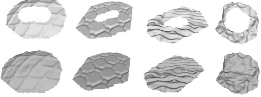
Fig. 11. Example of relief patterns ranging from regular, irregular to stochastic patterns.(Top row) Input surfaces with big holes on them. (Bottom row) Surfaces are filled with relief information extracted from the input surfaces.
All models uses distance metric DistHn in Eq. (9) with the weight setting to 0.5. The number of points, k, used as nearest neighbor is three.
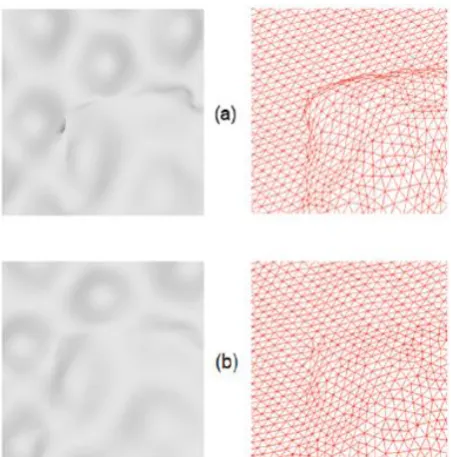
Figure 1 and Figure 11 show a wide range of relief patterns that can be completed using the proposed method. The orientation and direction of the relief pattern can be captured and synthesized by Laplacian signature as seen in Fig. 11. Figure 12 shows the input meshes with known relief patterns. The small neighborhood size of 7x7 (30% of the relief pattern size) and 11x11 (70% of the relief pattern size) do not fairly capture the relief pattern of the inputs surface. These surfaces require the neighborhood size of at least 13x13 (100% of the relief pattern size) in order to faithfully capture the relief detail.
Fig. 12. (a) The input surface with hole. (b) The neighborhood size of 30% of the repeatable relief pattern is used for the surface completion. (c) use the neighborhood size of 70% of the relief pattern. (d) use the neighborhood size of 100% of the relief patterns.
Figure 13 shows the dragon model with multiple relief patterns. The model does not contain large exemplar area. Thus, it is a little challenging for the algorithm to extract the pattern from the available surface. However, the proposed method can produce satisfying result.
[image:12.595.82.498.502.685.2]with the number of vertices of the hole area and the offset area. The running time also scales linearly with the number of sampling points used for the Laplacian surface signature. For surface with 5,000 vertices, the computation time is around 125 seconds. And for the surface with 10,000 vertices, the computation time is around 500 seconds.
[image:13.595.80.539.143.322.2]Fig. 13. Dragon model with multiple relief patterns contains many holes on the surface. Surface completion using Laplacian transform are performed on every holes on the model. The variable settings on all of these holes completion are the same.
[image:13.595.120.475.374.717.2]Fig. 15. The geometric deviation (c, f) and the normal deviation (d, g) of input surfaces.
Figure 14 shows the reproducibility of our method for various models. The results indicate that the holes can be completed with the geometric detail similar to the original surrounding surfaces.
The goal of this research is to produce the filled surface that have similar in visual appearance with the original surface. The synthesized patterns do not need to be the exact replicate of the original patterns. In Fig. 15, surface (a) is the original surface. Surface (b) is the surface completed with relief transfer using the proposed algorithm. Surface (e) is the smoothly filled surface. Obviously, when compare with the original surface (a), surface (b) should have less error or less deviation than surface (e). However, it turn out that this is not the case when using traditional surface comparison metrics. Image (c) and (d) show the Geometric deviation of 3.67 and Normal deviation of 1.60 respectively when comparing surface (b) to surface (a). Image (f) and (g) show the Geometric deviation of 4.21 and Normal deviation of 1.33 when comparing surface (e) to surface (a). The results indicate that the errors value from these matrices do not reflect the visual appearance of the comparing surfaces. The error metrics generally used for the mesh comparison, such as Geometric deviation or Normal deviation [26], cannot be used in this kind of task.
In addition, these metrics are transformation variant. The two surfaces with the same geometric pattern but are different in transformation, such as translation or rotation, would have great error.
6.
Discussion and Conclusions
This research proposes an algorithm to fill the hole on non-smooth surfaces using the available surface context. The algorithm can handle surface with relief patterns such as near-regular patterns, irregular patterns and stochastic patterns. This work would have a great benefit to surface acquisition process. The users do not need to spend a great amount of time repairing the scanned models. Another strong point of the proposed method is that no modification is done on the original surface. The preservation of the surface characteristics is crucial in application such as archiving ancient objects.
The quality of the coarse mesh can determine the quality of the result filled surface. If the mesh is not smooth enough, the relief pattern may not be clearly detectable. In addition, if the height of the relief pattern is too low, the Laplacian representation of the relief mesh may contain too much noise. This situation complicates the algorithm to detect the pattern of the surface. The author would like to explore geometric metrics that can be used to guide the smoothing process. Surface may not have to be smoothed evenly and isotropically. Some points of the surface may need more smoothing that the others.
[image:14.595.113.482.83.307.2]Most of the time the results from scanning devices contain surface fragments. It will be very useful to extend the proposed method to handle hole with isles. To handle hole with isles, many parts of the algorithm require modification. Active contour based methods may be more suitable for smooth hole completion than minimum surface area method. The available surface information of the fragments can be used as guidance when transferring relief pattern from the offset region. However, working with these fragments can introduce many difficulties. For example, each isle can have its own holes. Laplacian coordinates computed from the isles boundary are not accurate. It may be easier to design the algorithm if some losses in geometric detail of these fragments are acceptable.
Acknowledgements
This work was supported by The Royal Golden Jubilee Ph.D. Program Scholarship.
References
[1] M. Pauly, N. Mitra, J. Giesen, M. Gross, and L. Guibas, “Example-based 3D scan completion,” in
Proceedings of Symposium on Geometry Processing, 2005.
[2] R. Schnabel, P. Degener, and R. Klein, “Completion and reconstruction with primitive shapes,” in
Computer Graphics Forum, vol. 28, no. 2, pp. 503-512, 2009.
[3] A. Sharf, M. Alexa, and D. Cohen, “Context based surface completion,” ACM Transaction on Graphics, 2004.
[4] T. Breckon and R. Fisher, “Three-dimensional relief surface completion via nonparametric techniques,”
IEEE Transaction on Pattern Analysis and Machine Intelligence, 2008.
[5] R. Sumner and J. Popovic, “Deformation transfer for triangle meshes,” in Proceedings of ACM SIGGRAPH, 2004.
[6] M. Botsch, R. Sumner, M. Pauly, and M. Gross, “Deformation transfer for detail-preserving surface editing,” in Proceedings of Vision, Modeling, and Visualization, 2006.
[7] L. Wei, S. Lefebvre, V. Kwatra, and G. Turk, “State of the art in example-based texture synthesis,” in “Eurographics 2009,” State of the Art Report, EG-STAR, 2009.
[8] P. Liepa, “Filling holes in meshes,” in Proceedings of Symposium on Geometry Processing, 2003.
[9] J. Davis, S. Marschner, M. Garr, and M. Levoy, “Filling holes in complex surfaces using volumetric diffusion,” in Proceeding of the 1st International Symposium on 3D Data Processing, Visualization and Transmission, 2002.
[10] A. Sharf, T. Lewiner, G. Shklarski, S. Toledo, and D. Cohen, “Interactive topology-aware surface reconstruction,” in Proceedings of ACM SIGGRAPH, 2007.
[11] H. Xie, K. Mcdonell, and H. Qin, “Surface reconstruction of noisy and defective data sets,”
Visualization, pp. 259-266, 2004.
[12] S. Park, X. Guo, H. Shin, and H. Qin, “Surface completion for shape and appearance,” the Visual Computer, vol. 22, no. 3, pp. 168-180, 2006.
[13] G. Bendels, R. Schnabel, and R. Klein, “Detail-preserving surface inpainting,” in Proceedings International Symposium on Virtual Reality, Archaeology and Cultural Heritage, 2005.
[14] G. Turk, “Texture synthesis on surfaces,” in Proceedings of ACM SIGGRAPH, 2001.
[15] L. Wei and M. Levoy, “Texture synthesis over arbitary manifold surfaces,” in Proceedings of ACM SIGGRAPH, 2001.
[16] L. Ying, A. Hertzmann, H. Biermann, and D. Zorin, “Texture and shape synthesis on surfaces,” in
Proceedings of Eurographics Workshop on Rendering, 2001.
[17] S. Zelinika and M. Garland, “Interactive texture synthesis on surfaces using jump maps,” in Proceedings of Eurographics Symposium on Rendering, 2003.
[18] O. Sorkine, “Differential representations for mesh processing,” in Computer Graphics Forum, vol. 25, no. 4, pp. 789-807, 2006.
[19] M. Meyer, M. Desbrun, P. Shcroder, and A. Barr, “Discrete differential geometry operators for triangulated 2-manifolds,” Visualization and Mathematics, 2003.
[21] D. Zorin, P. Schroder, and W. Sweldens, “Interactive multiresolution mesh editing,” in Proceedings of ACM SIGGRAPH, 1997.
[22] I. Guskov, W. Sweldens, and P. Schroder, “Multi-resolution signal processing for meshes,” in
Proceedings of ACM SIGGRAPH, 1999, pp. 325-334.
[23] M. Desbrun, M. Meyer, P. Schroder, and A. Barr, “Implicit fairing of irregular meshes using diffusion and curvature flow,” in Proceedings of ACM SIGGRAPH, 1999, pp. 317-324.
[24] A. A. Efros and T. K. Leung, “Texture synthesis by non-parametric sampling,” in the Proceedings of IEEE International Conference on Computer Vision, vol. 2, 1999, pp. 1033-1038.
[25] S. Toledo. (2003). Taucs: A library of sparse linear solvers [Online]. Available: http://www.tau.ac.il/ stoledo/taucs/.