Determination of forcing functions in the wave equation. Part II: the time-dependent case

This is a repository copy of Determination of forcing functions in the wave equation. Part II: the time-dependent case.

White Rose Research Online URL for this paper: http://eprints.whiterose.ac.uk/92048/

Version: Accepted Version

Article:

Hussein, SO and Lesnic, D (2016) Determination of forcing functions in the wave equation. Part II: the time-dependent case. Journal of Engineering Mathematics, 96 (1). pp. 135-153. ISSN 0022-0833

https://doi.org/10.1007/s10665-015-9786-x

[email protected] https://eprints.whiterose.ac.uk/ Reuse

Unless indicated otherwise, fulltext items are protected by copyright with all rights reserved. The copyright exception in section 29 of the Copyright, Designs and Patents Act 1988 allows the making of a single copy solely for the purpose of non-commercial research or private study within the limits of fair dealing. The publisher or other rights-holder may allow further reproduction and re-use of this version - refer to the White Rose Research Online record for this item. Where records identify the publisher as the copyright holder, users can verify any specific terms of use on the publisher’s website.

Takedown

If you consider content in White Rose Research Online to be in breach of UK law, please notify us by

This is a Determination of forcing functions in the wave equation. Part II: the time-dependent case

Article:

! ∀ ! # ∃%&∋() # ∗ + ,

− .. ∗ / 0 1 + + 2 ∗ .∀∀3 &&%%/& 44 ∃.

− )

5 + ∋& ∋&&6 ∋& (/&∋(/76 /5

promoting access to

Determination of forcing functions in the wave equation.

Part II: the time-dependent case

S.O. Hussein and D. Lesnic

Department of Applied Mathematics, University of Leeds, Leeds LS2 9JT, UK

E-mails: [email protected], [email protected]

Abstract.

equation is investigated. This is a natural continuation of Part I (J. Eng. Maths 2015, this volume), where the space-dependent force identification has been considered. The ad-ditional data is given by a space integral average measurement of the displacement. This linear inverse problem has a unique solution, but it is still ill-posed since small errors in the input data cause large errors in the output solution. Consequently, when the input data is contaminated with noise we use the Tikhonov regularization method in order to obtain a stable solution. The choice of the regularization parameter is based on the L-curve method. Numerical results show that the solution is accurate for exact data and stable for noisy data.

Keywords:

1

Introduction

The wave equation governs many physical problems such as the vibrations of a spring or membrane, acoustic scattering, etc. When it comes to mathematical modeling probably the most investigated are the direct and inverse acoustic scattering problems, see e.g. [1]. On the other hand, inverse source/force problems for the wave equation have been less investigated. External force estimation consists of the inverse process of identifying the applied loadings from the output measurements of the system responses and can be experienced in many engineering applications dealing with wave, wind, seismic, explosion, or noise excitations, [2]. It is the objective of this study to investigate such an inverse force problem for the hyperbolic wave equation. The forcing function is assumed to depend only upon the single time variable in order to ensure uniqueness of the solution. The identification of a space-dependent forcing function has been investigated elsewhere, see [3]- [6], [7, Sect. 8.2] and Part I of this topic submitted in the companion paper [8]. The theoretical basis for our numerical investigation is given in [7, Sect. 9.2], where the existence and uniqueness of solution of the inverse time-dependent force function for the wave equation have been established. However, no numerical results were presented and it is the main purpose of our study to develop an efficient numerical solution for this linear, but ill-posed inverse problem.

2

Mathematical Formulation

The governing equation for a vibrating bounded structure Ω ⊂Rn_{, n= 1,2,3, acted upon}

by a forceF(x, t) is given by the wave equation

utt(x, t) = c2∇2u(x, t) +F(x, t), (x, t)∈Ω×[0, T], (1)

where T > 0 is a given time, u(x, t) represents the displacement and c > 0 is the wave speed of propagation. For simplicity, we assume that c is a constant, but we can also let

c be a positive smooth function depending on the space variable x. We also assume that the boundary ∂Ω is smooth enough. Equation (1) has to be solved subject to the initial conditions

u(x,0) =u0(x), x∈Ω, (2)

ut(x,0) = v0(x), x∈Ω, (3)

whereu0 andv0 represent the initial displacement and velocity, respectively. On the

bound-ary of the structure∂Ωwe can prescribe Dirichlet, Neumann or Robin boundary conditions. Due to the linearity of equation (1) and of the direct and inverse force problems which are investigated we can assume, for simplicity, that these boundary conditions are homogeneous. We can therefore take

u(x, t) = 0, (x, t)∈∂Ω×[0, T], (4)

or,

∂u

∂n+σ(x)u= 0, (x, t)∈∂Ω×[0, T], (5)

where n is the outward unit normal to the boundary ∂Ω and σ is a sufficiently smooth function. Equation (5) includes the Neumann boundary condition which is obtained for

σ ≡0.

If the forceF(x, t)is given, then the equations above form a direct well-posed problem for the displacement u(x, t). However, if the force function F(x, t) cannot be directly observed it hence becomes unknown and then clearly, the above set of equations is not sufficient to determine the pair solution (u(x, t), F(x, t)). Then, we can consider the additional integral measurement

Z

Ω

ω(x)u(x, t)dx=ψ(t), t∈[0, T], (6)

where ω is a given weight function, and further assume that

F(x, t) =f1(x, t)h(t) +f2(x, t), (x, t)∈Ω×[0, T], (7)

where f1(x, t) and f2(x, t) represent known forcing function components and h(t) is an

un-known time-dependent coefficient that is sought. Physically, the expression (6) represents a space average measurement of the displacement. Also, if one takes the weight function ω to mimic an approximation to the Dirac delta distribution δ(x−x0), where x0 ∈ Ω is fixed,

then (6) becomes a pointwise measurement of the displacement, namely, u(x₀, t) =ψ(t) for

t ∈ [0, T]. The assumption (7) is needed in order to ensure the unique solvability of the inverse force problem under investigation, see Theorems 1 and 2 below. We finally men-tion that instead of (7) one can seek a space-wise component g(x) of the force in the form

F(x, t) =f1(x, t)g(x) +f2(x, t), and this case has been thoroughly investigated elsewhere in

For the definition and notation of the functional spaces involved in the sequel and related concepts, see Chapter 1 of [7].

We assume that the input data satisfy the regularity conditions

u0 ∈W˚21(Ω), v0 ∈L2(Ω), ψ ∈C2[0, T], f1, f2 ∈C([0, T];L2(Ω)), ω∈W˚21(Ω), (8)

the compatibility conditions

Z

Ω

u0(x)ω(x)dx=ψ(0),

Z

Ω

v0(x)ω(x)dx=ψ′(0), (9)

and the identifiability condition

Z

Ω

f1(x, t)ω(x)dx6= 0, t∈[0, T]. (10)

Based on Rellich’s theorem that W˚1

2(Ω) is compactly embedded into L2(Ω), we can also

consider stronger regularity conditions than (8), namely,

u0 ∈W22(Ω)∩W˚21(Ω), v0 ∈W˚21(Ω), ψ ∈C2[0, T], f1, f2 ∈C([0, T]; ˚W21(Ω)),

ω∈W˚1

2(Ω). (11)

Then, collecting the statements of corollaries 9.2.1 and 9.2.2 of [7], we obtain the following unique solvability theorem of the inverse problem (1)-(4), (6) and (7).

Theorem 1. (i) If the input data satisfy conditions (8)-(10), then there exists a unique

solution (u(x, t), h(t)) of the inverse problem (1)-(4), (6) and (7) in the class of functions

u∈C([0, T];W₂1(Ω))∩C1([0, T];L2(Ω)), h∈C[0, T]. (12)

(ii) If the input data satisfy conditions (9)-(11), then there exists a unique solution(u(x, t), h(t))

of the inverse problem (1)-(4), (6) and (7) in the class of functions

u∈C2([0, T];L2(Ω))∩C1([0, T];W21(Ω))∩C([0, T];W22(Ω)), h∈C[0, T]. (13)

When we consider the Robin boundary condition (5), we replace the regularity conditions (8) by the slightly weaker assumptions

u0 ∈W21(Ω), v0 ∈L2(Ω), ψ ∈C2[0, T], f1, f2 ∈C([0, T];L2(Ω)), ω∈W˚21(Ω), (14)

and (11) by

u0 ∈W22(Ω), v0 ∈W21(Ω), ψ ∈C2[0, T], f1, f2 ∈C([0, T];W21(Ω)), ω∈W˚21(Ω),

∂fi

∂n +σfi

∂Ω×[0,T]

= 0, i= 1,2,

∂u0

∂n +σu0

∂Ω

= 0. (15)

Then, collecting the statements of corollaries 9.2.3 and 9.2.4 of [7], we obtain the following unique solvability theorem of the inverse problem (1)-(3), (5)-(7).

Theorem 2. (i) If the input data satisfy conditions (9), (10) and (14), then there

functions (12).

(ii) If the input data satisfy conditions (9),(10) and (15), then there exists a unique solution

(u(x, t), h(t)) of the inverse problem (1)-(3), (5)-(7) in the class of functions (13).

Theorems 1 and 2 establish the existence and uniqueness of solution of the inverse force problems (1)-(4), (6), (7) and (1)-(3), (5)-(7), respectively. Although these theorems ensure that a unique solution exists, the following example shows that this solution does not depend continuously upon the input data.

Example of instability. Consider the one-dimensional case, i.e. n = 1 and Ω = (0, π),

and the inverse problem given by equations (1)-(4), (6) and (7) in the form

utt(x, t) =uxx(x, t) +f1(x, t)h(t) +f2(x, t), (x, t)∈(0, π)×(0, T), (16)

u(x,0) =u0(x) = 0, ut(x,0) =v0(x) =

x(x−π)

n1/2 , x∈(0, π), (17)

u(0, t) = u(π, t) = 0, t ∈[0, T], (18)

ψ(t) =

Z π

0

ω(x)u(x, t)dx= π

5_sin(nt)

30n3/2 , t ∈[0, T], (19)

where n∈N∗ _and

ω(x) = x(x−π), f1(x, t) =−x(x−π), f2(x, t) =−

2 sin(nt)

n3/2 .

One can observe that conditions (8)-(10) are satisfied and that the analytical solution of the inverse problem (16)-(19) is given by

u(x, t) = sin(nt)x(x−π)

n3/2 , (20)

h(t) = n1/2sin(nt). (21)

Then, one can easily see that, as n → ∞ all the input data (17)-(19) tend to zero, but the output time-dependent component (21) becomes unbounded and oscillatory. This shows that the inverse problem under investigation is ill-posed by violating the stability condition with respect to errors in the data (19). On the other hand, as pointed out by one of the referees, stability could be restored if one assumes higher regularity for the measured input data (19); for example, the data (input) and unknown (output) become of comparable norms if ψ is measured in H2_{[0, T](or C}2_{[0, T]) and thenh is in L}2_{[0, T] (or C[0, T]).}

3

Numerical Solution of the Direct Problem

In this section, we consider the direct initial boundary value problem (1)-(4), for simplicity, in one-dimension, i.e. n = 1and Ω = (0, L)withL >0, when the forceF(x, t)is known and the displacement u(x, t) is to be determined, namely,

utt(x, t) = c2uxx(x, t) +F(x, t), (x, t)∈(0, L)×[0, T], (22)

u(x,0) = u0(x), ut(x,0) =v0(x), x∈[0, L], (23)

u(0, t) =u(L, t) = 0, t∈[0, T]. (24)

The discrete form of this problem is as follows. We divide the solution domain (0, L)× (0, T) into M and N subintervals of equal lengths ∆x and ∆t, where ∆x = L/M and

∆t = T /N. We denote by ui,j = u(xi, tj), where xi = i∆x, tj = j∆t, and Fi,j := F(xi, tj)

for i = 0, M, j = 0, N. Then, a central-difference approximation to equations (22)-(24) at the mesh points (xi, tj) = (i∆x, j∆t) of a rectangular mesh covering the solution domain (0, L)×(0, T) is, [11],

ui,j+1 =r2ui+1,j+ 2(1−r2)ui,j +r2ui−1,j−ui,j−1+ (∆t)2Fi,j,

i= 1,(M −1), j = 1,(N −1), (25)

ui,0 =u0(xi), i= 0, M ,

ui,1−ui,−1

2∆t =v0(xi), i= 1,(M −1), (26)

u0,j = 0, uM,j = 0, j = 0, N , (27)

where r =c∆t/∆x. Expression (25) represents an explicit FDM formula which is stable if

r ≤ 1, giving approximate values for the solution at mesh points along t = 2∆t,3∆t, ..., as soon as the solution at the mesh points along t= ∆t has been determined. Puttingj = 0in equation (25) and using (26), we obtain

ui,1 =

1 2r

2_u

0(xi+1) + (1−r2)u0(xi) + 1 2r

2_u

0(xi−1) + (∆t)v0(xi) + 1 2(∆t)

2_F

i,0,

i= 1,(M−1). (28)

The desired output (6) is calculated using the trapezium rule

ψ(tj) =

∆x

2 ω0u0,j+ 2 M−1

X i=1

ωiui,j+ωMuM,j

! = ∆x

M−1

X i=1

ωiui,j, j = 1, N , (29)

where ωi =ω(xi)for i= 0, M, and use has been made of (27).

The normal derivative at the boundary is calculated using the second-order finite-difference approximations

−∂u

∂x(0, tj) = −

4u1,j−u2,j−3u0,j

2∆x =

u2,j−4u1,j

2∆x , ∂u

∂x(L, tj) =

3uM,j −4uM−1,j+uM−2,j

2∆x =

uM−2,j−4uM−1,j

2∆x , j = 1, N , (30)

4

Numerical Solution of the Inverse Problem

We now consider the inverse initial boundary value problem (2)-(4), (6) and (7), in one-dimension, i.e. n= 1 and Ω = (0, L), when both the force h(t)and the displacement u(x, t)

are to be determined, from the governing equation

utt(x, t) =c2uxx(x, t) +f1(x, t)h(t) +f2(x, t), (x, t)∈(0, L)×[0, T], (31)

subject to the initial and boundary conditions (23) and (24), and the measurement (6). In discretised finite-difference form equations (23), (24) and (31) recast as equations (26), (27), and

ui,j+1−(∆t)2f1i,jhj =r2ui+1,j+ 2(1−r2)ui,j+r2ui−1,j−ui,j−1+ (∆t)2f2i,j,

i= 1,(M −1), j = 1,(N −1), (32)

where f1i,j := f1(xi, tj), hj := h(tj) and f2i,j := f2(xi, tj). Putting j = 0 in equation (32)

and using (26), we obtain

ui,1−

1 2(∆t)

2_f

1i,0h0 =

1 2r

2_u

0(xi+1) + (1−r2)u0(xi) + 1 2r

2_u

0(xi−1) + (∆t)v0(xi)

+1 2(∆t)

2_f

2i,0, i= 1,(M −1). (33)

In practice, the additional observation (29) comes from measurement which is inherently contaminated with errors. We therefore model this by replacing the exact data ψ(tj) with

the noisy data

ψǫ(tj) = ψ(tj) +ǫj, j = 1, N , (34)

where(ǫj)j=1,N areN random noisy variables generated (using the MATLAB routine ’normrd’)

from a Gaussian normal distribution with mean zero and standard deviationσ˜ given by

˜

σ=p× max

t∈[0,T]|ψ(t)|, (35)

where prepresents the percentage of noise.

Assembling equations (29), (32) and (33), and using (26) and (27), the discretised inverse problem reduces to solving a global linear, but ill-conditioned system of (M −1)×N +N

equations with (M −1)×N +N unknowns. Since this system is linear we can eliminate the unknowns ui,j for i = 1,(M −1), j = 1, N, to reduce the problem to solving an

ill-conditioned system of N equations withN unknowns of the generic form

Ah =bǫ, (36)

where the right-hand sidebǫ includes the noisy data (34).

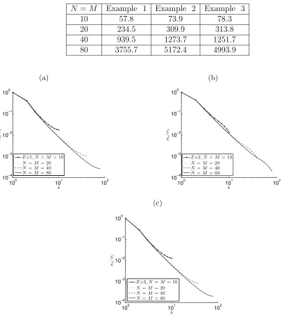
For the examples that will be considered in the next section, the condition numbers of the matrix A in (36) (calculated using the command cond(A) in MATLAB) given in Table 1 are of O(102_{) to O(10}4_{) for M =N ∈ {10,20,40,80}, respectively. These large condition}

numbers indicate that the system of equations (36) is ill-conditioned. The ill-conditioning nature of the matrixA can also be revealed by plotting its normalised singular valuesσk/σ1

Table 1: Condition number of the matrixA.

N =M Example 1 Example 2 Example 3

10 57.8 73.9 78.3

20 234.5 309.9 313.8

40 939.5 1273.7 1251.7 80 3755.7 5172.4 4993.9

(a)

100 101 102

10−4 10−3 10−2 10−1 100

k

σk

/

σ

1

E x1, N=M= 10 N=_M= 20 N=M= 40 N=M= 80

(b)

100 101 102

10−4 10−3 10−2 10−1 100

k

σk

/

σ

1

E x2, N=M= 10 N=M= 20 N=_M= 40 N=M= 80

(c)

100 101 102

10−4 10−3 10−2 10−1 100

k

σk

/

σ

1

E x3, N=M= 10

N=M= 20

N=M= 40

N=_M= 80

Figure 1: Normalised singular values σk/σ1 for k= 1, M, for Examples 1-3.

5

Numerical Results and Discussion

In all examples we take, for simplicity, c=L=T = 1.

5.1

Example 1

As a typical test example, consider first the direct problem (22)-(24) with the input data

u(x,0) =u0(x) =x(x−1), ut(x,0) =v0(x) = 0, x∈[0,1], (37)

u(0, t) = 0, u(1, t) = 0, t ∈[0,1], (38)

The exact solution of this direct problem is given by

u(x, t) = x(x−1)(t3+ 1), (x, t)∈[0,1]×[0,1]. (40)

For the weight function

ω(x) = x(x−1), x∈(0,1), (41)

the desired output (6) is given by

ψ(t) =

Z 1

0

ω(x)u(x, t)dx= 1

30(t

3_{+ 1), t∈[0,1]. (42)}

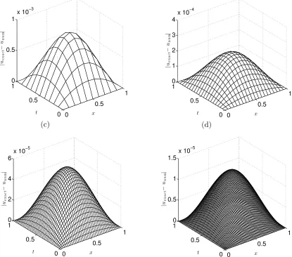
The absolute errors between the numerical and exact solutions for u(x, t) at interior points are shown in Figure 2 and one can observe that an excellent agreement is obtained. From this figure it can also be observed that the errors are reduced by a factor of 4(= 22_),

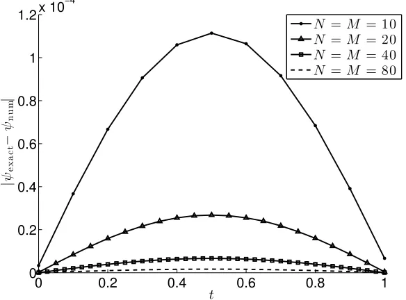
when N is doubled, which confirms that the numerical results are correct, and accurate up to second-order, due to the second-order FDM used. Figure 3 also gives the corresponding absolute errors for ψ(t). From this figure it can be seen that the numerical results are in very good agreement with the exact solution (42), and that convergence is rapidly achieved as N =M increases.

The inverse problem given by equations (31) with f1(x, t) = 6x(x−1) and f2(x, t) =

−2(t3 _{+ 1), (37), (38) and (42) is considered next. One can easily check that conditions}

(a) 0 0.5 1 0 0.5 1 0 0.5 1

x 10−3

x t | u e x a c t − un u m | (b) 0 0.5 1 0 0.5 1 0 1 2 3 4

x 10−4

x t | ue x a c t − u n u m | (c) 0 0.5 1 0 0.5 1 0 2 4 6

x 10−5

x t | u e x a c t − un u m | (d) 0 0.5 1 0 0.5 1 0 0.5 1 1.5

x 10−5

x t | u e x a c t − un u m |

Figure 2: The absolute errors between the exact (40) and numerical displacement u(x, t)

0 0.2 0.4 0.6 0.8 1 0

0.2 0.4 0.6 0.8 1 1.2x 10

−4

t

|

ψ

e

x

a

c

t

−

ψn

u

m

|

N =M = 10

N =M = 20

N =M = 40

N =M = 80

Figure 3: The absolute error between the exact (42) and numerical ψ(t)obtained by solving the direct problem with N =M ∈ {10,20,40,80}, for Example 1.

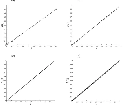
5.1.1 Exact Data

(a)

0 0.1 0.2 0.3 0.4 0.5 0.6 0.7 0.8 0.9 0

0.1 0.2 0.3 0.4 0.5 0.6 0.7 0.8 0.9 1

t

h

(

t

)

(b)

0 0.1 0.2 0.3 0.4 0.5 0.6 0.7 0.8 0.9 1 0

0.1 0.2 0.3 0.4 0.5 0.6 0.7 0.8 0.9 1

t

h

(

t

)

(c)

0 0.1 0.2 0.3 0.4 0.5 0.6 0.7 0.8 0.9 1 0

0.1 0.2 0.3 0.4 0.5 0.6 0.7 0.8 0.9 1

t

h

(

t

)

(d)

0 0.1 0.2 0.3 0.4 0.5 0.6 0.7 0.8 0.9 1 0

0.1 0.2 0.3 0.4 0.5 0.6 0.7 0.8 0.9 1

t

h

(

t

)

(a) 0 0.5 1 0 0.5 1 0 2 4 6

x 10−5

x t | u e x a c t − un u m | (b) 0 0.5 1 0 0.5 1 0 1 2 3 4

x 10−6

x t | u e x a c t − un u m | (c) 0 0.5 1 0 0.5 1 0 1 2 3

x 10−7

x t | ue x a c t − u n u m | (d) 0 0.2 0.4 0.6 0.8 1 0 0.2 0.4 0.6 0.8 1 0 0.2 0.4 0.6 0.8 1 1.2 1.4

x 10−8

x t | ue x a c t − u n u m |

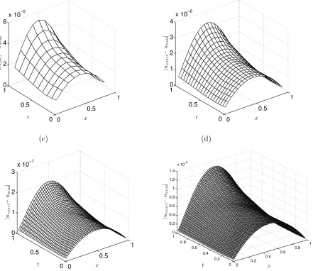
Figure 5: The absolute errors between the exact (40) and numerical displacement u(x, t)

obtained with N =M =(a) 10, (b) 20, (c) 40, and (d) 80, and no regularization, for exact data, for the inverse problem of Example 1.

5.1.2 Noisy Data

In order to investigate the stability of the numerical solution we include some p∈ {1,3,5}%

noise into the input data (29), as given by equation (34). The numerical solution for h(t)

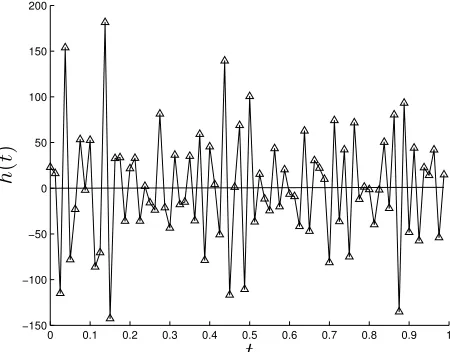
obtained with N = M = 80 and no regularization has been found highly oscillatory and unstable, as shown in Figure 6. In order to deal with this instability we employ the Tikhonov regularization which gives the regularized solution, [9],

h_λ = (ATA+λDT_kDk)−1ATbǫ, (43)

where Dk is the regularization derivative operator of order k ∈ {0,1,2} and λ ≥ 0 is the

regularization parameter. The regularization derivative operator Dk imposes continuity, i.e.

classC0 _{fork= 0, first-order smoothness, i.e. classC}1_{fork= 1, or second-order smoothness,}

i.e. classC2 _{for k = 2, namely D}

0 0.1 0.2 0.3 0.4 0.5 0.6 0.7 0.8 0.9 1 −150

−100 −50 0 50 100 150 200

t

h

(

t

)

Figure 6: The exact (—) solution forh(t)in comparison with the numerical solution (—∆—) for N =M = 80, p= 1% noise, and no regularization, for the inverse problem of Example 1.

D1 =

   

1 −1 0 0 ... 0 0 1 −1 0 ... 0

... ... ... ... ... ...

0 0 ... 0 1 −1    

, D2 =

   

1 −2 1 0 0 ... 0 0 1 −2 1 0 ... 0

... ... ... ... ... ... ...

0 0 ... 0 1 −2 1    

.

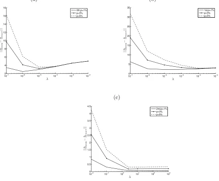
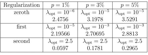
Including regularization we obtain the solution (43) whose accuracy error, as a function of λ, is plotted in Figure 7. The minimum points λopt and the minimal errors are listed in

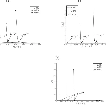
Table 2. From Figure 7 and Table 2 it can be seen that the errors decrease as the amount of noisepdecrease and that the 2nd-order regularization produces much smaller errors than the zeroth and 1st-order regularisations. However, these arguments and conclusions cannot be used for choosing the regularization parameter λ in the absence of an analytical (exact) solution being available. Then, one possible criterion for choosing λ is given by the L-curve method, [10], which plots the residual norm||Ah_λ−bǫ||versus the solution norm||Dkhλ||for

various values of λ. This is shown in Figure 8 for various values of λ ∈ {10−8_,10−7_{, ...,10}3_}

and for p ∈ {1,3,5}% noisy data. The portion to the right of the curve corresponds to large values of λ which make the solution oversmooth, whilst the portion to the left of the curve corresponds to small values of λ which make the solution undersmooth. The compromise is then achieved around the corner region of the L-curve where the aforemen-tioned portions meet. Figure 8 shows that this corner region includes the values around

{λ0th = 10−6, λ1st = 10−5, λ2nd = 2.5} for p = 1%, {λ0th = 10−5, λ1st = 10−3, λ2nd = 2.5}

for p = 3%, and {λ0th = 10−5, λ1st = 10−3, λ2nd = 2.5} for p = 5%, which were previously

obtained from Figure 7.

Figure 9 shows the regularized numerical solution for h(t) obtained with λopt given in

(a)

10−7 10−6 10−5 10−4 10−3 10−2 2

4 6 8 10 12 14 16 18

λ

||

hn

u

m

−

he

x

a

c

t

||

0th,p=1% p=3% p=5%

(b)

10−7 10−6 10−5 10−4 10−3 10−2 0

5 10 15 20 25 30 35

λ

||

hn

u

m

−

he

x

a

c

t

||

1st,p=1% p=3% p=5%

(c)

10−2 10−1 100 101 102 103 0

0.5 1 1.5 2 2.5 3 3.5 4 4.5

λ

||

hn

u

m

−

he

x

a

c

t

||

2nd,p=1% p=3% p=5%

(a)

0 0.01 0.02 0.03 0.04 0.05 0.06 0

10 20 30 40 50 60 70 80 90

||Ahλ−b

ǫ

||

||

hλ

||

p=1% p=3% p=5%

λ=10−5 λ=10−5

λ=10−6

(b)

0.0050 0.01 0.015 0.02 0.025 0.03 0.035 0.04 0.045

2 4 6 8 10 12 14 16 18

||Ah_λ−bǫ

||

||

h

′||λ

p=1%

p=3%

p=5%

λ=10−5 λ=10−3 λ=10

−3

(c)

0 0.01 0.02 0.03 0.04 0.05 0.06 0.07 0.08 0.09 0

0.01 0.02 0.03 0.04 0.05 0.06

||Ah_λ

−b

ǫ

||

||

h

′′||λ

p=1% p=3% p=5%

λ_=2.5

(a)

0 0.2 0.4 0.6 0.8 1

−0.2 0 0.2 0.4 0.6 0.8 1

t

h

(

t

)

exact

p= 1%,λ_{0 th= 10}−6

p= 3%,λ_{0 th= 10}−5

p=5%,λ_{0 th= 10}−5

(b)

0 0.2 0.4 0.6 0.8 1

−0.2 0 0.2 0.4 0.6 0.8 1

t

h

(

t

)

exact

p= 1%,λ_{1 st= 10}−5

p= 3%,λ_{1 st}= 10−3

p= 5%,λ_{1 st= 10}−3

(c)

0 0.2 0.4 0.6 0.8 1

0 0.2 0.4 0.6 0.8 1

t

h

(

t

)

exact

p= 1%,λ_{2 n d}= 2.5

p= 3%,λ_{2 n d= 2}.5

p= 5%,λ_{2 n d= 2}.5

Figure 9: The exact (—) solution for h(t) in comparison with the regularized numerical solution (43), for N =M = 80,p∈ {1,3,5}% noise, for the inverse problem of Example 1.

Table 2: The error norms ||h_num − h_exact|| for various order regularization methods and percentages of noise p, for the inverse problem of Example 1.

Regularization p= 1% p= 3% p= 5%

zeroth λopt = 10−6 λopt = 10−5 λopt = 10−5

2.4756 3.1978 3.5291

first λopt = 10−5 λopt = 10−3 λopt = 10−3

2.19566 2.70695 2.8813

second λopt = 2.5 λopt = 2.5 λopt = 2.5

0.0597 0.1781 0.2965

5.2

Example 2

As another example, consider first the direct problem (23), (24) and (31) with the input data (38),

u(x,0) = u0(x) = 0, ut(x,0) =v0(x) = 0, x∈[0,1], (44)

and

h(t) =

(

t if 0≤t≤ 1₂,

1−t if 1₂ < t≤1. (46)

Remark that in this example, the expression (46) has a triangular shape, being continuous but non-differentiable at the peak t = 1/2. Furthermore, an explicit analytical solution for the displacement u(x, t) does not seem readily available.

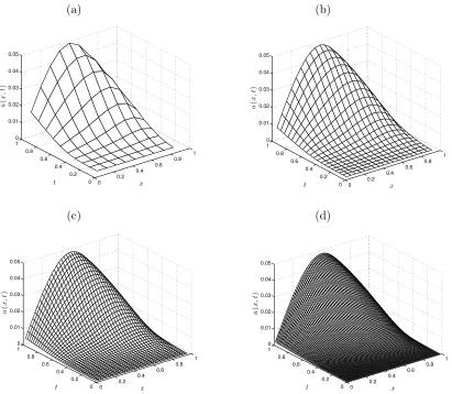
The numerical FDM solutions for the displacement u(x, t) at interior points are shown in Figure 10, whilst the desired output (6) forω given by (41) is presented in Figure 11.

(a) 0 0.2 0.4 0.6 0.8 1 0 0.2 0.4 0.6 0.8 1 0 0.01 0.02 0.03 0.04 0.05 x t u ( x , t ) (b) 0 0.2 0.4 0.6 0.8 1 0 0.2 0.4 0.6 0.8 1 0 0.01 0.02 0.03 0.04 0.05 x t u ( x , t ) (c) 0 0.2 0.4 0.6 0.8 1 0 0.2 0.4 0.6 0.8 1 0 0.01 0.02 0.03 0.04 0.05 x t u ( x , t ) (d) 0 0.2 0.4 0.6 0.8 1 0 0.2 0.4 0.6 0.8 1 0 0.01 0.02 0.03 0.04 0.05 x t u ( x , t )

0 0.1 0.2 0.3 0.4 0.5 0.6 0.7 0.8 0.9 1 −7

−6 −5 −4 −3 −2 −1

0x 10 −3

t

ψ

(

t

)

N₌M_{= 5}

N=M= 10

N=M= 20

N=M= 40

N₌M_{= 80}

Figure 11: Numerical solution for the integral (6), obtained by solving the direct problem with various N =M ∈ {5,10,20,40,80}, for Example 2.

The inverse problem given by equations (31), (38), (44), (45) and (6) with ψ numerically simulated by solving the direct problem using the FDM with N = M = 160 is considered next. Remark that from (41) and (45) it follows that the identifiability condition (10) is satisfied. The solution of the inverse problem is given exactly for h(t) by equation (46) and numerically foru(x, t) illustrated for sufficiently large N =M such as 80, in Figure10(d).

5.2.1 Exact Data

(a)

0 0.1 0.2 0.3 0.4 0.5 0.6 0.7 0.8 0.9 0

0.05 0.1 0.15 0.2 0.25 0.3 0.35 0.4 0.45 0.5

t

h

(

t

)

(b)

0 0.1 0.2 0.3 0.4 0.5 0.6 0.7 0.8 0.9 1 0

0.05 0.1 0.15 0.2 0.25 0.3 0.35 0.4 0.45 0.5

t

h

(

t

)

(c)

0 0.1 0.2 0.3 0.4 0.5 0.6 0.7 0.8 0.9 1 0

0.05 0.1 0.15 0.2 0.25 0.3 0.35 0.4 0.45 0.5

t

h

(

t

)

(d)

0 0.1 0.2 0.3 0.4 0.5 0.6 0.7 0.8 0.9 1 0

0.05 0.1 0.15 0.2 0.25 0.3 0.35 0.4 0.45 0.5

t

h

(

t

)

Figure 12: The exact (—) solution (46) for h(t) in comparison with the numerical solution (—∆—) for various N =M = (a) 10, (b) 20, (c)40, and (d) 80, and no regularization, for exact data, for the inverse problem of Example 2.

5.2.2 Noisy Data

In order to investigate the stability of the numerical solution we include some p∈ {1,3,5}%

noise into the input data (29), as given by equation (34). The numerical solution for h(t)

obtained with N = M = 80 and no regularization has been found highly oscillatory and unstable similar to that obtained in Figure 6 and therefore is not presented. In order to deal with this instability we employ the Tikhonov regularization which gives the stable solution (43) provided that an appropriate regularization parameter λ is chosen. The accuracy error of this regularized solution, as a function of λ, is plotted in Figure 13. The minimum points

λopt and the minimal errors are listed in Table 3. The L-curve criterion for choosing λ

produces an L-corner, as it also happened in Example 1. This is shown in Figure 14 for various values of λ∈ {10−9_,10−8_{, ...,10} and for p∈ {1,3,5}%noisy data. Figure 14 shows}

that this corner region includes the values around {λ0th = 10−6, λ1st = 10−6, λ2nd = 10−5}

for p = 1%, λ0th,1st,2nd = 10−4 for p = 3%, and λ0th,1st,2nd = 10−2 for p = 5%, which were

previously obtained from Figure 13.

Figure 15 shows the regularized numerical solution forh(t)obtainedλopt given in Table 3

(a)

10−9 10−8 10−7 10−6 10−5 10−4 10−3

0 5 10 15 20 25 30

λ

||

hn

u

m

−

he

x

a

c

t

||

0th,p=1% p=3% p=5%

(b)

100−7 10−6 10−5 10−4 10−3 10−2 10−1

0.5 1 1.5 2 2.5 3 3.5 4

λ

||

hn

u

m

−

he

x

a

c

t

||

1st,p=1% p=3% p=5%

(c)

10−5 10−4 10−3 10−2 10−1 100 101 0

0.5 1 1.5 2 2.5 3

λ

||

hn

u

m

−

he

x

a

c

t

||

2nd,p=1% p=3% p=5%

Figure 13: The accuracy error ||h_num − h_exact||, as a function of λ, for M = N = 80,

(a)

0 0.005 0.01 0.015 0.02 0.025

0 5 10 15 20 25 30

||Ahλ−b

ǫ

||

||

hλ

||

p=1% p=3% p=5%

λ₌₁₀−6

λ₌₁₀−5

(b)

0 0.001 0.002 0.003 0.004 0.005 0.006 0.007 0.008 0.009 0.01 0

0.2 0.4 0.6 0.8 1 1.2 1.4

||Ahλ−b

ǫ

||

||

h

′||λ

p=1% p=3% p=5%

λ=10−4

(c)

0.5 1 1.5 2 2.5 3 3.5 4

x 10−3 0

0.01 0.02 0.03 0.04 0.05 0.06 0.07 0.08 0.09

||Ah_λ

−b

ǫ

||

||

h

′′||λ

p=1% p=3% p=5%

λ₌₁₀−2

λ=10−2

(a)

0 0.1 0.2 0.3 0.4 0.5 0.6 0.7 0.8 0.9 1 −0.1

0 0.1 0.2 0.3 0.4 0.5

t

h

(

t

)

exact

p= 1%,λ_{0 th}= 10−6

p= 3%,λ_{0 th}= 10−6

p= 5%,λ_{0 th= 10}−5

(b)

0 0.1 0.2 0.3 0.4 0.5 0.6 0.7 0.8 0.9 1 −0.1

0 0.1 0.2 0.3 0.4 0.5

t

h

(

t

)

exact

p= 1%,λ_{1 st= 10}−4

p= 3%,λ_{1 st}= 10−4

p= 5%,λ_{1 st= 10}−4

(c)

0 0.1 0.2 0.3 0.4 0.5 0.6 0.7 0.8 0.9 1 −0.2

−0.1 0 0.1 0.2 0.3 0.4 0.5

t

h

(

t

)

exact

p= 1%,λ2 n d= 10−2

p= 3%,λ_{2 n d= 10}−2

p= 5%,λ2 n d= 10−2

Figure 15: The exact solution (46) for h(t) in comparison with the regularized numerical solution (43), for N =M = 80,p∈ {1,3,5}% noise, for the inverse problem of Example 2.

Table 3: The error norms ||h_num − h_exact|| for various order regularization methods and percentages of noise p, for the inverse problem of Example 2.

Regularization p= 1% p= 3% p= 5%

zeroth λopt = 10−6 λopt = 10−6 λopt = 10−5

0.2008 0.3388 0.3925

first λopt = 10−4 λopt = 10−4 λopt = 10−4

0.1909 0.2365 0.3125

second λopt = 10−2 λopt = 10−2 λopt = 10−2

0.2475 0.3641 0.4980

5.3

Example 3

We finally consider the Robin boundary condition (5). Let the initial conditions (23) be given by

u(x,0) = u0(x) = sin

3π

4 x+

π

8

and the Robin boundary conditions (5) be given by

−∂u

∂x(0, t) +

3π

4 cot π

8

u(0, t) = 0, ∂u

∂x(1, t)−

3π

4 cot

7π

8

u(1, t) = 0, t ∈[0,1]. (48)

We also take in (31),

f1(x, t) = sin

3π

4 x+

π

8

, f2(x, t) =

9π2

16 sin

3π

4 x+

π

8

, x∈(0,1), (49)

h(t) = 6t+9π

2

16 t

3_{, t ∈[0,1]. (50)}

Then, the exact solution of the direct problem (31), (47) and (48) is given by

u(x, t) = (t3+ 1) sin

3π

4 x+

π

8

, (x, t)∈[0,1]×[0,1]. (51)

For the weight function (41), the desired output (6) is given by

ψ(t) =

Z 1

0

ω(x)u(x, t)dx= 32

27π3

3πsinπ 8

−8 cosπ 8

(t3+ 1), t ∈[0,1]. (52)

The FDM requires slight modifications from the Dirichlet boundary condition (38) when implementing the Robin boundary conditions (48), but this poses no difficulty, [11]. We simply approximate the x-derivatives at x = 0 and 1 using central finite differences by introducing fictitious points outside the space domain [0,1] and apply the general FDM scheme (25) for j = 0 and N, as well.

(a) 0 0.5 1 0 0.5 1 0 0.005 0.01 0.015 0.02 x t | ue x a c t − u n u m | (b) 0 0.5 1 0 0.5 1 0 1 2 3 4 5

x 10−3

x t | u e x a c t − un u m | (c) 0 0.5 1 0 0.5 1 0 0.5 1 1.5

x 10−3

x t | ue x a c t − u n u m | (d) 0 0.5 1 0 0.5 1 0 1 2 3 4

x 10−4

x t | u e x a c t − un u m |

Figure 16: The absolute errors between the exact (51) and numerical displacement u(x, t)

0 0.2 0.4 0.6 0.8 1 0

0.2 0.4 0.6 0.8 1 1.2 1.4 1.6x 10

−3

t

|

ψe

x

a

c

t

−

ψn

u

m

|

N =M = 10

N =M = 20

N =M = 40

N =M = 80

Figure 17: The absolute error between the exact (52) and numericalψ(t)obtained by solving the direct problem with N =M ∈ {10,20,40,80}, for Example 3.

The inverse problem given by equations (31), (47), (48) and (52) is considered next. One can easily check that conditions (9), (10) and (14) are satisfied and hence Theorem 2 ensures the existence of a unique solution in the class of functions (12). In fact, the exact solution is given by equations (50) and (51).

The discretised inverse problem reduces to solving a global linear, but ill-conditioned system of (M+ 1)×N+N equations with (M + 1)×N +N unknowns. Since this system is linear we can eliminate the unknowns ui,j fori= 0, M, j = 1, N, as in (36), to reduce the

problem to solving an ill-conditioned system of N equations with N unknowns.

5.3.1 Exact Data

(a)

0 0.1 0.2 0.3 0.4 0.5 0.6 0.7 0.8 0.9

0 1 2 3 4 5 6 7 8 9 10

t

h

(

t

)

(b)

0 0.1 0.2 0.3 0.4 0.5 0.6 0.7 0.8 0.9 1 −2

0 2 4 6 8 10 12

t

h

(

t

)

(c)

0 0.1 0.2 0.3 0.4 0.5 0.6 0.7 0.8 0.9 1 −2

0 2 4 6 8 10 12

t

h

(

t

)

(d)

0 0.1 0.2 0.3 0.4 0.5 0.6 0.7 0.8 0.9 1 −2

0 2 4 6 8 10 12

t

h

(

t

)

(a) 0 0.5 1 0 0.5 1 0 0.005 0.01 x t | ue x a c t − u n u m | (b) 0 0.5 1 0 0.5 1 0 1 2 3

x 10−3

x t | ue x a c t − u n u m | (c) 0 0.5 1 0 0.5 1 0 2 4 6

x 10−4

x t | u e x a c t − un u m | (d) 0 0.5 1 0 0.5 1 0 0.5 1 1.5

x 10−4

x t | u e x a c t − un u m |

Figure 19: The absolute errors between the exact (51) and numerical displacement u(x, t)

obtained with N =M =(a) 10, (b) 20, (c) 40, and (d) 80, and no regularization, for exact data, for the inverse problem of Example 3.

5.3.2 Noisy Data

In order to investigate the stability of the numerical solution we include some p∈ {1,3,5}%

noise into the input data (29), as given by equation (34). The numerical solution for h(t)

obtained with N = M = 80 and no regularization has been found highly oscillatory and unstable similar to that obtained in Figure 6 and therefore is not presented. In order to deal with this instability we employ the zeroth order, first-order and second-order Tikhonov regularization, similar to Section 5.1.2 for Example 1. The accuracy error of the regularized solution (43), as a function of λ, is plotted in Figure 20. The minimum points λopt and

the minimal errors are listed in Table 4. The L-curve criterion for choosing λ produces an L-corner, as it also happened in Example 1. This is shown in Figure 21 for various values of

λ ∈ {10−8_,10−7_{, ...,10} and for p ∈ {1,3,5}% noisy data. Figure 21 shows that this corner}

region includes the values around{λ0th = 10−7, λ1st = 5×10−5, λ2nd = 5×10−2}forp= 1%,

{λ0th = 10−6, λ1st = 10−4, λ2nd = 10−1} for p = 3%, and {λ0th = 10−5, λ1st = 10−4, λ2nd =

10−1_{}for p= 5%, as previously predicted from Figure 20.}

Figure 22 shows the regularized numerical solution for h(t) obtained with λopt given

regularization. As in Example 1, one can see that the second-order regularization method produces the most stable and accurate numerical results.

(a)

10−8 10−7 10−6 10−5 10−4 10−3 10−2 10−1 0

50 100 150 200 250 300 350

λ

||

hn

u

m

−

he

x

a

c

t

||

0th,p=1% p=3% p=5%

(b)

10−6 10−5 10−4 10−3 10−2 10−1

20 25 30 35 40 45 50 55 60 65

λ

||

hn

u

m

−

he

x

a

c

t

||

1st,p=1% p=3% p=5%

(c)

10−3 10−2 10−1 100 101

0 5 10 15 20 25 30 35

λ

||

hn

u

m

−

he

x

a

c

t

||

2nd,p=1% p=3% p=5%

(a)

0 0.1 0.2 0.3 0.4 0.5 0.6 0.7

0 50 100 150 200 250 300 350

||Ahλ−b

ǫ

||

||

hλ

||

p=1% p=3% p=5%

λ=10−7

λ=10−6

λ=10−5

(b)

0 0.05 0.1 0.15 0.2 0.25

0 2 4 6 8 10 12 14 16

||Ahλ−b

ǫ

||

||

h

′||λ

p=1% p=3% p=5%

λ=5×10−5

(c)

0 0.1 0.2 0.3 0.4 0.5 0.6 0.7

0 0.1 0.2 0.3 0.4 0.5 0.6 0.7

||Ahλ−b

ǫ

||

||

h

′′||λ

p=1% p=3% p=5%

λ=10−1

(a)

0 0.1 0.2 0.3 0.4 0.5 0.6 0.7 0.8 0.9 1 −6

−4 −2 0 2 4 6 8 10 12

t

h

(

t

)

exact

p= 1%,λ_{0th= 10}−7

p= 3%,λ_0th= 10−6

p= 5%,λ_0th= 10−5

(b)

0 0.1 0.2 0.3 0.4 0.5 0.6 0.7 0.8 0.9 1 −4

−2 0 2 4 6 8 10 12

t

h

(

t

)

exact

p= 1%,λ_1st= 5×10−5

p= 3%,λ_1st= 10−4

p= 5%,λ_1st= 10−4

(c)

0 0.1 0.2 0.3 0.4 0.5 0.6 0.7 0.8 0.9 1 −2

0 2 4 6 8 10 12

t

h

(

t

)

exact

p= 1%,λ_{2nd= 5×10}−2

p= 3%,λ_2nd= 10−1

p= 5%,λ_2nd= 10−1

Figure 22: The exact solution (50) for h(t) in comparison with the numerical regularized solution (43), for N =M = 80,p∈ {1,3,5}% noise, for the inverse problem of Example 3.

Table 4: The error norms ||h_num − h_exact|| for various order regularization methods and percentages of noise p, for the inverse problem of Example 3.

Regularization p= 1% p= 3% p= 5%

zeroth λopt = 10−7 λopt = 10−6 λopt = 10−5

24.4962 29.5028 33.5244

first λopt = 5×10−5 λopt = 10−4 λopt = 10−4

23.0137 24.4016 26.1625

second λopt = 5×10−2 λopt = 10−1 λopt = 10−1

1.5648 2.1300 3.3874

6

Conclusions

Numerical simulations for a wide range of external forces have been performed in order to test the validity of the present investigation. The obtained results indicate that the method can accurately and stably recover the unknown force. Although the numerical method and results have been presented for the one-dimensional time-dependent wave equation a similar FDM can easily be extended to higher dimensions. Future work will consist in investigating the nonlinear inverse problem in which the unknown forcef(u)depends on the displacement

u.

Acknowledgments

S.O. Hussein would like to thank the Human Capacity Development Programme (HCDP) in Kurdistan for their financial support in this research. The comments and suggestions made by the referees are gratefully acknowledged.

References

[1] Colton, D. and Kress, R. Inverse Acoustic and Electromagnetic Scattering Theory, 3rd edn., Springer Verlag, New York, 2013.

[2] Huang, C.-H. An inverse non-linear force vibration problem of estimating the external forces in a damped system with time-dependent system parameters, Journal of Sound and Vibration, 242, 749-765, 2001.

[3] Cannon, J.R. and Dunninger, D.R. Determination of an unknown forcing function in a hyperbolic equation from overspecified data, Annali di Matematica Pura ed Applicata, 1, 49-62, 1970.

[4] Engl, H.W., Scherzer, O. and Yamamoto, M. Uniqueness and stable determination of forcing terms in linear partial differential equations with overspecified boundary data, Inverse Problems, 10, 1253-1276, 1994.

[5] Hussein, S.O. and Lesnic, D. Determination of a space-dependent source function in the one-dimensional wave equation, Electronic Journal of Boundary Elements,12, 1-26, 2014.

[6] Yamamoto, M.Stability, reconstruction formula and regularization for an inverse source hyperbolic problem by a control method, Inverse Problems,11, 481-496, 1995.

[7] Prilepko, A. I., Orlovsky, D. G. and Vasin, I. A. Methods for Solving Inverse Problems

in Mathematical Physics, Marcel Dekker, Inc., New York, 2000.

[8] Hussein, S.O. and Lesnic, D. Determination of forcing functions in the wave equation. Part I: the space-dependent case, Journal of Engineering Mathematics, (accepted). http://arxiv.org/abs/1410.6475

[9] Philips, D.L. A technique for the numerical solution of certain integral equations of the first kind, Journal of the Association for Computer Machinery, 9, 84-97, 1962.

[10] Hansen, P.C. The L-curve and its use in the numerical treatment of inverse problems, in Computational Inverse Problems in Electrocardiology, (ed. P. Johnston), WIT Press, Southampton, 119-142, 2001.