A MUSIC-based method for SSVEP signal processing

(1)

This is a repository copy of

A MUSIC-based method for SSVEP signal processing

.

White Rose Research Online URL for this paper:

http://eprints.whiterose.ac.uk/125857/

Version: Accepted Version

Article:

Chen, K, Liu, Q, Ai, Q et al. (3 more authors) (2016) A MUSIC-based method for SSVEP

signal processing. Australasian Physical and Engineering Sciences in Medicine, 39 (1). pp.

71-84. ISSN 0158-9938

https://doi.org/10.1007/s13246-015-0398-6

© Australasian College of Physical Scientists and Engineers in Medicine 2016. This is an

author produced version of a paper published in Australasian Physical and Engineering

Sciences in Medicine. The final publication is available at Springer via

https://doi.org/10.1007/s13246-015-0398-6. Uploaded in accordance with the publisher's

self-archiving policy.

eprints@whiterose.ac.uk https://eprints.whiterose.ac.uk/

Reuse

Unless indicated otherwise, fulltext items are protected by copyright with all rights reserved. The copyright exception in section 29 of the Copyright, Designs and Patents Act 1988 allows the making of a single copy solely for the purpose of non-commercial research or private study within the limits of fair dealing. The publisher or other rights-holder may allow further reproduction and re-use of this version - refer to the White Rose Research Online record for this item. Where records identify the publisher as the copyright holder, users can verify any specific terms of use on the publisher’s website.

Takedown

If you consider content in White Rose Research Online to be in breach of UK law, please notify us by

(2)

A MUSIC-based Method for SSVEP Signal Processing

Kun Chen1,3_{, Quan Liu}2,3,*_{, Qingsong Ai}2,3_{, Zude Zhou}1,3_{, Sheng Quan Xie}4_{, Wei Meng}2,3 1_{School of Mechanical and Electronic Engineering, Wuhan University of Technology, Wuhan 430070, China}

2_{School of Information Engineering, Wuhan University of Technology, Wuhan 430070, China} 3_{Key Laboratory of Fiber Optic Sensing Technology and Information Processing, Ministry of Education,}

Wuhan 430070, China

4_{Department of Mechanical Engineering, The University of Auckland, Auckland 1010, New Zealand} *_{Corresponding author: email: quanliu@whut.edu.cn; Tel: +862787655520; Fax: +862787655520}

Abstract 1

The research on brain computer interfaces (BCIs) has 2

become a hotspot in recent years because it offers benefit to 3

disabled people to communicate with the outside world. 4

Steady state visual evoked potential (SSVEP)-based BCIs 5

are more widely used because of higher signal to noise ratio 6

(SNR) and greater information transfer rate (ITR) compared 7

with other BCI techniques. In this paper, a multiple signal 8

classification (MUSIC)-based method was proposed for 9

multi-dimensional SSVEP feature extraction. 2-second data 10

epochs from four electrodes achieved excellent accuracy 11

rates including idle state detection. In some asynchronous 12

mode experiments, the recognition accuracy reached up to 13

100%. The experimental results showed that the proposed 14

method attained good frequency resolution. In most 15

situations, the recognition accuracy was higher than 16

canonical correlation analysis (CCA), which is a typical 17

method for multi-channel SSVEP signal processing. Also, a 18

virtual keyboard was successfully controlled by different 19

subjects in an unshielded environment, which proved the 20

feasibility of the proposed method for multi-dimensional 21

SSVEP signal processing in practical applications. 22

23

Keywords 24

brain computer interface (BCI), steady state visual evoked 25

potential (SSVEP), multiple signal classification (MUSIC), 26

feature extraction. 27

1 INTRODUCTION 28

A brain computer interface (BCI) is a communication 29

system that does not depend on the brain’s normal output

30

pathways of peripheral nerves and muscles[1] . The ultimate 31

goal of a BCI is to create a specialized interface that allows 32

an individual with severe motor disabilities to have effective 33

control of devices such as computers, speech synthesizers, 34

assistive appliances and prostheses[2]. 35

Electroencephalography (EEG) is most commonly used 36

for BCIs because it has advantages of portability and ease of 37

use. A steady state visual evoked potential (SSVEP) is a 38

periodic response to a visual stimulus modulated at a 39

frequency higher than 6 Hz[3] (or 4Hz[4] ). It can be 40

recorded from the scalp as a nearly sinusoidal oscillatory 41

waveform with the same fundamental frequency as the 42

stimulus, and often includes some higher harmonics. The 43

amplitude and phase characteristics of SSVEPs depend upon 44

the stimulus intensity and frequency. SSVEP-based BCIs are 45

becoming a research hotspot because it has many advantages 46

over other BCI systems including a higher signal to noise 47

ratio (SNR), and faster information transfer rate (ITR). It 48

also does not require intensive training [5]. 49

A variety of methods have been developed and used for 50

feature extraction for SSVEP-based BCIs[6]. Fourier-based 51

transform methods are mostly used for power spectrum 52

density analysis (PSDA). Most research used them to 53

compute the accumulative power at the stimulus frequencies 54

and their harmonics for frequency-coded SSVEPs. Or the 55

average power centered on the stimulus frequency was 56

calculated[7] . An important advantage of Fourier-based 57

transforms is their simplicity and small computation time. 58

However, the time window length of SSVEP signals needs to 59

be long enough to enhance the frequency resolution of FFT 60

when the sampling frequency is confirmed. This might limit 61

practical applications because it has a lower information 62

transfer rate (ITR) [8]. Additionally, a larger window length 63

could lead to classification errors during the changing of 64

stimuli. The studies [8-10] all used wavelet analysis to 65

estimate power at relevant frequency points. A key problem 66

with applying wavelet analysis is how to choose an 67

appropriate mother wavelet to attain good performance. 68

Although the wavelet analysis is better for non-stationary 69

signal processing compared with Fourier transform, it is 70

developed based on Fourier transform, which is fit for 71

processing linear signals. New methods suitable for 72

non-linear and non-stationary signal processing are needed. 73

In this case, Hilbert Huang transform (HHT) is adopted in 74

previous studies [11,12]. HHT has more stability than FFT, 75

which means the recognition accuracy will not change 76

greatly when the data length varies. Although HHT can be 77

well used for non-linear and non-stationary SSVEPs, its 78

computation time is higher compared with Fourier transform. 79

All the methods discussed above were commonly employed 80

to process single channel SSVEPs. Signals from 81

multi-channel EEG are less affected by noise than signals 82

from a unipolar or bipolar system. The combination of 83

signals collected from different channels (electrodes) is also 84

referred to as spatial filtering. Typical methods like 85

minimum energy combination (MEC) and maximum 86

contrast combination (MCC) are the most commonly utilized 87

[13-16]. Another method named canonical correlation 88

analysis (CCA) can be employed to extract features from a 89

different viewpoint. It computes the correlation of two 90

multi-variable datasets [17]. Paper [18] used CCA to 91

recognize SSVEP for the first time. A further comparison 92

between the CCA and PSDA method was done by Hakvoort 93

(3)

2 et al. [19], which showed that CCA had better performance. 94

Spatial filtering methods have the advantage of combining 95

signal pre-processing and feature extraction together. 96

In this paper, a new method based on multiple signal 97

classification (MUSIC) was proposed for feature extraction 98

of multi-dimensional SSVEPs. One of the typical 99

applications of MUSIC is to solve the problem of harmonic 100

retrieval for one-dimensional signals. The principle of using 101

MUSIC for target frequency recognition of 102

multi-dimensional SSVEPs was explained in detail. Also, a 103

criterion used to determine the number of eigenvectors 104

constructing the signal subspace for power spectrum 105

estimation was proposed. The method was verified with both 106

simulated and real SSVEP data. Experiments in synchronous 107

and asynchronous modes were conducted. The results show 108

that MUSIC achieved a good frequency resolution. 109

Meanwhile, it is capable of suppressing noise because it 110

decomposes the original data into signal subspace and noise 111

subspace. Compared with CCA, MUSIC is more flexible, as 112

the number of eigenvectors constructing the signal subspace 113

is adjustable. The recognition accuracy was better than CCA 114

in most situations. Finally, the proposed method was 115

successfully utilized for users to control a virtual keyboard in 116

an unshielded environment. 117

This paper is organized as follows: methods including the 118

principle of MUSIC, the procedure of SSVEP signal 119

processing and the setup of experiments are explained in 120

Section 2. The experimental results are illustrated in Section 121

3. Discussion and conclusions are presented in Section 4 and 122

Section 5. 123

2 MATERIALS AND METHODS 124

2.1 Multiple Signal Classification for SSVEP Signal 125

Processing 126

MUSIC was first proposed by R. O. Schmidt in 1979[20]. 127

It is often used to solve the problem of harmonic retrieval 128

and direction of arrival. The data model [21] can be 129

expressed as follows. 130 ) ( ) 2 exp( ) ( 1 n w j nf j a n x k p

k k k

  







(1)

131

Here, ( )w n is additive noise. a_k, f_k and k represent the 132

amplitude, frequency and phase respectively.pdenotes the 133

number of harmonics. 134

The SSVEP signal is a periodic response to the stimulus 135

frequency and its harmonics, which can be modeled using 136

the above formula. Actually, many other methods like MEC, 137

MCC or CCA employ similar data models to represent 138

SSVEPs. The model includes sum of stimulus frequencies 139

and noise. They are typically used for multi-channel signals. 140

In this situation, the data model should be defined as: 141

)]

(

),...,

(

),

(

[

)

(

n

x

1

n

x

2

n

x

n

XX



num (2) 142

Here, numis the number of channels. It is assumed that the 143

data includes both signals and noises, which are independent 144

of each other[22] . Thus, the covariance matrix can be 145

decomposed into signal and noise components. 146

As mentioned before, the typical use of MUSIC method is 147

to solve the problem of harmonic retrieval for 148

one-dimensional signals. The principle of using MUSIC for 149

multi-dimensional SSVEP signal processing is illustrated as 150

follows. 151

A simulated signal according to Formula (1) is generated 152 as: 153 ) 512 , 1 ( * 5 . 15 ) / * 871 . 5 * 2 sin( * 10 ) / * 384 . 5 * 2 sin( * 20 * 5 . 0 ) ( randn f n f n n x S S   



(3) 154

Where, the value of f_S is 256, and n ranges from 1 to 155

512. It can be seen that there are two harmonic components 156

with frequencies of 5.384 Hz and 5.871 Hz for the simulated 157

signal. The spatial smoothing method which reconstructs 158

one-dimensional signals to multi-dimensional signals, is 159

usually employed to analyze the signal as Formula (3). The 160

reconstructed signal is an N M dimension matrix. As for 161

the MUSIC method, N means the number of snapshots, and 162

M means the number of arrays. The reconstructed 163

multi-dimensional signal can be represented by a matrix X. 164                  ) 1 ( ... ) 1 ( ) ( ... ... ... ... ) 1 ( ... ) 3 ( ) 2 ( ) ( ... ) 2 ( ) 1 ( N M x N x N x M x x x M x x x

X

(4)

165

The first row of the new matrix includes 166 ) ( ), 1 ( ),..., 2 ( ), 1

( x xM xM

x  ; the second row of the new 167

matrix includes x(2),x(3),...,x(M),x(M1), and so on. 168

The last row includes

169 ) 1 ( ), 2 ( ),..., 1 ( ),

(N xN xMN xMN

x . Because the

170

total number of sampling points for the original signal x(n) 171

is 512, the maximum sum of M and N is 513. 172

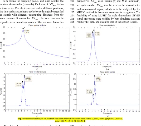
The values of M and N were adjusted to reconstruct the 173

signal. The result of power spectral analysis for the new 174

multi-dimensional signal with various values of M and

N

175

is illustrated as Fig. 1. 176

It is seen in Fig. 1(a) only one harmonic component of 177

5.632 Hz is recognized. While in Fig. 1(b), Fig. 1(c) and Fig. 178

1(d) , two harmonic components of 5.376 Hz and 5.888 Hz 179

can be recognized, which are quite close to the harmonic 180

components of the original signal represented by Formula 181

(3). For real SSVEP signals, the recognition accuracy of 182

target frequencies doesn’t normally need to be 0.001 Hz. The 183

harmonic recognition effect became better with the value of 184

M increasing in experiments. However, the result would 185

not improve any more if Mincreased to some extent. 186

For the matrix X, each row can be seen as a time series. 187

Compared the next row with the last low, the next one can be 188

regarded as a unit-time delay time series of the last one. The 189

real SSVEP signal as in Formula (2) can be also represented 190

by a matrix XX_new. 191              ) ( ... ) 2 ( ) 1 ( ... ... ... ... ) ( ... ) 2 ( ) 1 ( ) ( ... ) 2 ( ) 1 ( 2 2 2 1 1 1 sam x x x sam x x x sam x x x XX num num num

new

(5)

(4)

sa m means the sampling points, and num denotes the 193

number of electrodes (channels). Each row of XX_new is also 194

a time series. For electrodes are laid at different positions, 195

the time series according to each electrode might be regarded 196

as signals with different transmitting distances from the 197

same sources. It means for XX_new, the next row can be 198

regarded as a time-delay series of the last one. From this 199

perspective, XX_new as in Formula (5) and X in Formula (4) 200

are quite similar. XX_new can be seen as the reconstructed 201

multi-dimensional signal, which is to be analyzed by the 202

MUSIC method for harmonic components recognition. The 203

feasibility of using MUSIC for multi-dimensional SSVEP 204

signal processing were verified by both simulated data and 205

real SSVEP data, and it can be seen in the section Results. 206

207

(a)

(b) 208

209

(c) (d) 210

Fig. 1 Power spectral analysis for reconstructed signal with various values of M and N. (a)M=5, N=507; (b)M=200, N=312;

211

(c)M=500, N=12; (d) M=508, N=4. 212

213

The detailed computation procedure is described as 214

follows: 215

(1)Assume that the original SSVEP signal is a samnum 216

dimension matrix. sa m and num represent the number of 217

sampling points and the number of channels. 218

(2)As explained above, sa m can be seen as M in 219

Formula (4), and num can be seen as N.The covariance 220

matrix R_XX of the new matrix XX_newis a samsam 221

dimensional matrix. Compute the eigenvalues d₁

,

d2

, ...,

222

sam

d and eigenvectors V₁

,

V2

,...,

Vsamof the covariance 223

matrix. 224

(3)The eigenvectors corresponding to the k largest 225

eigenvalues constitute the signal subspace, while the 226

remaining eigenvectors constitute the noise subspace. How 227

to confirm the value of

k

is also discussed in this paper. 228

(4)Use the signal subspace or the noise subspace for power 229

spectrum estimation as follows. 230

) ) (

/( 1 )

( FT

T i i F I SS a a

f

P  

(6)

231

) ) ( /( 1 )

( F

T o o T

F N N a a

f

P 

(7)

232

I is a samsam dimensional unit matrix. S_i and 233

o

N represent the signal and the noise subspace with 234

dimensions of samk and sam(samk)

.

aF is a 235

sam



1 dimensional matrix. The value of each element is: 236

) ,..., 2 , 1 ( , )

, 1

( i e *( 1)* i sam

a j i order

F  



 

(8) 237

1 ) /

(  

round f f

order

(9) 238

s order 2**f*order/f



(10)

239

Here, fsis the sampling frequency, f is the frequency 240

interval, and f is the target frequency.. 241

The value of kcan be defined as a constant which is 242

[image:4.612.40.575.53.529.2]

(5)

4 a threshold. It needs time to adjust the value to maximize the 244

recognition results. Inspired by the principle of minimum 245

energy combination [14], which is another important 246

technique for spatial filtering, the number of eigenvalues is 247

chosen corresponding to the following equation. 248

k

i

d

i

/

1



0 .

01 ,



1 ,

2 ,

3 ,...,

(11) 249

Here, d₁is the largest eigenvalue of the covariance matrix 250

and d₁

,

d₂ till d_k are sorted in descending order. Only 251

these eigenvectors whose corresponding eigenvalues are no 252

less than 1% of the largest eigenvalue are classified as the 253

signal subspace for spectrum estimation. 254

The SSVEP signal processing usually includes data 255

pre-processing, feature extraction and feature classification. 256

In our research, a low-pass filter with a cut-off frequency of 257

30 Hz and a 50 Hz notch filter were used for pre-processing. 258

The original data were segmented into epochs for feature 259

extraction via the MUSIC method. The basic idea is to 260

compute the power values at stimulus frequencies. As for 261

feature classification, the frequency corresponding to the 262

maximum power value was recognized as the target one. If 263

there are n stimulus frequencies which are f₁, f₂ till f_n. 264

The power value P( f) corresponding to each frequency is 265

computed as shown in Formula (6). And then the target 266

frequency is confirmed as the following formulas. 267

)) ( max( arg

arg P f

f_t _et (12) 268



n



et

t

arg



1 ,

2 ,...,

(13) 269

From the above two formulas, it can be seen that we should 270

focus on the magnitude relation of power values 271

corresponding to different stimulus frequencies, not the 272

absolute magnitude of a specific power value. Therefore, the 273

units of power values are not labeled in all figures in this 274

paper. 275

A dwell time, which means the state of one target kept for 276

a period of time, was employed to reduce the false positives. 277

The detailed explanations about this are given in the Results 278

and Discussion sections. 279

The recognition results were compared with the CCA 280

method in experiments. Here, the principle of CCA[23] is 281

briefly introduced. If there are two variables X and Y with 282

dimensions of p and q respectively. X and Y are 283

represented as X(X1,X2,...,Xp) and Y(Y1,Y2,...,Yq). 284

To find out the relation between X and Y, a linear 285

combination is applied to both X and Y. Two new 286

variables are generated which are 287 p pX a X a X a

U  1 1 2 2... and

288 q qY b Y b Y b

V 1 1 2 2... . Then the correlation coefficient 289

) , (U V corr



 between U and V is computed. 290

) ,..., ,

(a1 a2 ap

a and b(b1,b2,...,bq) are named 291

canonical variables when p has the largest value, and



is 292

the canonical correlation coefficient between X and Y . 293

If there are four stimulus frequencies used in practical 294

applications which are f₁, f₂, f₃ and f₄, four reference 295

signals should be constructed as follows: 296 ] ) * * 2 cos( ) * * 2 sin( [ 1 1 21 t f t f

X  _

(14) 297 ] ) * * 2 cos( ) * * 2 sin( [ 2 2 22 t f t f X  



(15)

298 ] ) * * 2 cos( ) * * 2 sin( [ 3 3 23 t f t f X  



(16)

299 ] ) * * 2 cos( ) * * 2 sin( [ 4 4 24 t f t f X  



(17)

300

If the original SSVEP data are denoted by X₁ , the 301

aforementioned CCA method is used to compute the 302

correlation coefficients ₁, ₂, ₃, ₄between X₁ and 303

21

X , X₂₂ , X₂₃ , X₂₄ . Then the target frequency is 304

dertermined according to the following formula. 305

}

4 ,

3 ,

2 ,

1 {

arg

)),

(

max(

arg



f

t

et



f

t et



(18)

306

It is noted that the reference signals only use the 307

fundamental harmonic components corresponding to 308

stimulus frequencies. The second or other harmonics can be 309

also used to calculate the correlation coefficients if 310

necessary. 311

2.2 Experimental Setup 312

As the signal and noise components of simulated data are 313

deterministic, the simulated data are suitable for method 314

verification. But the real SSVEP data are more persuasive to 315

prove that the proposed method can be used in practical 316

applications. So both simulated and real SSVEP data were 317

used in our experiments. 318

1) Simulated data 319

In experiments, four-channel data were generated. Each 320

channel includes two sine waves to simulate the harmonic 321

components of SSVEP and random noise. The frequencies of 322

two sine components are 5.384 and 5.871 Hz, respectively, 323

just like the harmonic components used in Formula (19). The 324

data are expressed as follows. 325                                             ) , 1 ( * 5 . 16 ) / * 871 . 5 * 2 sin( * 10 ) / * 384 . 5 * 2 sin( * 20 * 1 . 0 ); , 1 ( * 8 . 15 ) / * 871 . 5 * 2 sin( * 10 ) / * 384 . 5 * 2 sin( * 20 * 2 . 0 ); , 1 ( * 5 . 15 ) / * 871 . 5 * 2 sin( * 10 * 8 . 0 ) / * 384 . 5 * 2 sin( * 20 * 1 . 0 ); , 1 ( * 5 . 15 ) / * 871 . 5 * 2 sin( * 10 ) / * 384 . 5 * 2 sin( * 20 * 5 . 0 ] 4 ; 3 ; 2 ; 1 [ N ra ndn s f n s f n N ra ndn s f n s f n N ra ndn s f n s f n N ra ndn s f n s f n S S S S S         326 (19) 327

Here, f_s is the sampling frequency equal to 256 Hz. Nis 328

the total number of sampling points with a value of 512. n 329

represents each single sampling point ranging from 1 to 512. 330

(6)

frequency interval of two components is 0.487 Hz. It doesn’t

332

strictly meet the frequency resolution requirement for 333

traditional FFT method to estimate the spectrum, because the 334

resolution is computed as 0.5 Hz (fs/N256/512). Also, 335

both of the frequency points 5.384 and 5.871 are not located 336

on the FFT spectral lines. However, MUSIC can better 337

estimate the power values at these two points. It is shown in 338

the Results section. 339

2) Real SSVEP data 340

The stimulus panel contains four LED blocks each 341

measured as 2*2 cm. The distance between LED blocks and 342

the flickering frequencies are adjustable. The effects of these 343

parameters on experimental results are discussed in the 344

following section. 345

A Symtop UE-16B EEG amplifier was used in our 346

experiments as shown in Fig. 2. It has 16 channels and a USB 347

interface. The maximum sampling frequency can be adjusted 348

to 1000 Hz. A low-pass filter and a notch filter are 349

developed in the amplifier. 350

[image:6.612.305.574.47.441.2]

351

Fig. 2 UE-16B EEG amplifier and the experimental setup

352 353

In reality, the sampling frequency was set to 200 Hz, 354

because the frequency of EEG signals is usually lower than 355

100 Hz. Also, the stimuli frequencies used in experiments 356

are lower than 30 Hz. The choice of 200 Hz is reasonable. 357

Besides, an appropriate sampling frequency rather than a 358

higher frequency saves the computation time. The cut off 359

frequency of the low-pass filter was set to 30 Hz and the 50 360

Hz power line interference was removed by a notch filter. 361

All 16 channels (Fp1, Fp2, F3, F4, C3, C4, P3, P4, O1, O2, 362

F7, F8, T3, T4, T5, and T6) were utilized to acquire the 363

original EEG data in early stages. The number of channels 364

was reduced to 4 (P3, P4, O1, O2) in later experiments. Five 365

subjects (one female, four male) participated in the 366

experiments for performance analysis of related methods. 367

All of them have good eye vision. The average age is 25.4 368

years old. More subjects were asked to conduct the 369

experiment for real time control of a virtual keyboard. All 370

experiments were done in an unshielded environment. 371

Two different kinds of experiments were designed for the 372

five subjects, namely synchronous paradigm and 373

asynchronous paradigm. Regarding the synchronous one, 374

three sessions were conducted: (i) Only one of the four 375

stimuli was flickering. Subjects looked at the flickering one 376

for 40 seconds from the 20th second; (ii) Only one of the four 377

stimuli was flickering. Subjects looked at each area 378

corresponding to stimuli not flickering for 20 seconds 379

consecutively from the 20th second; (iii) Four stimuli were 380

flickering at the same time. Subjects looked at each one for 381

20 seconds consecutively from the 20th second. Labels were 382

used to indicate different experiment sessions as illustrated 383

in Fig. 3. As for the asynchronous paradigm, two following 384

sessions were carried out: (i) Subjects looked at different 385

stimuli according to a predefined number sequence. Once a 386

target was recognized, subjects turned to look at the next 387

stimulus. In our experiments, three number sequences were 388

defined as ‘1-2-3-4’, ‘1-3-2-4’ and ‘1-4-2-3’; (ii) Subjects 389

looked at stimuli randomly, and no sequence was defined 390

before the experiment. 391

392

Fig. 3 Explanation of SSVEP dataset labels in the synchronous mode

393 394

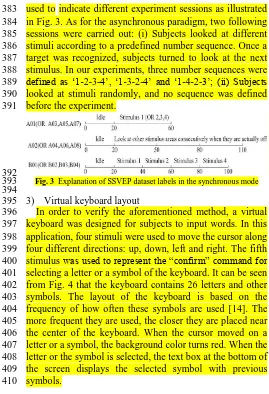
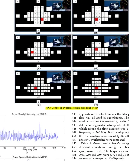
3) Virtual keyboard layout 395

In order to verify the aforementioned method, a virtual 396

keyboard was designed for subjects to input words. In this 397

application, four stimuli were used to move the cursor along 398

four different directions: up, down, left and right. The fifth 399

stimulus was used to represent the “confirm” command for 400

selecting a letter or a symbol of the keyboard. It can be seen 401

from Fig. 4 that the keyboard contains 26 letters and other 402

symbols. The layout of the keyboard is based on the 403

frequency of how often these symbols are used [14]. The 404

more frequent they are used, the closer they are placed near 405

the center of the keyboard. When the cursor moved on a 406

letter or a symbol, the background color turns red. When the 407

letter or the symbol is selected, the text box at the bottom of 408

the screen displays the selected symbol with previous 409

symbols. 410

3 RESULTS 411

3.1 Simulated Data Analysis 412

Fig. 5(a) illustrates the power spectrum obtained by 413

MUSIC method. The spectrum area around 6 Hz was 414

zoomed in as shown in Fig. 5(b). 415

It is obvious in Fig. 5(b) that two peaks appear at around 416

5.3 and 5.8 Hz, which are almost equal to the harmonic 417

components of the simulated data. Also, the spectral curve is 418

smooth in Fig. 5(b), which means a high frequency 419

resolution can be acquired. 420

3.2 Real SSVEP Data Analysis 421

For real SSVEP signals, MUSIC was utilized to calculate 422

the power at those stimulus frequency points. The stimulus 423

frequency corresponding to the maximum power value was 424

recognized as the target one. Taking the processing results of 425

dataset A03 as an example, as shown in Fig. 6, four curves 426

with different colors represent the power values of the four 427

stimulus frequencies (6, 7, 8, 9 Hz).The values 428

corresponding to the second stimulus are higher than the 429

other three after the 22nd seconds. The 2-second delay is 430

mainly caused by the response time when subjects changed 431

[image:6.612.43.281.279.360.2]

(7)

6 433

Fig. 4 Control of a virtual keyboard based on SSVEP

434

435

436

(a) 437

438

(b) 439

Fig. 5 Spectrum of the simulated data computed by MUSIC

440 441

which means SSVEP signals responding to one stimulus 442

have to keep for a period of time, was employed in real 443

applications in order to reduce the false positives. The dwell 444

time was adjusted in experiments. The CCA method was 445

used to compare the processing results. The original SSVEP 446

data were segmented into epochs of 400 sampling points, 447

which means the time duration was 2 seconds (sampling 448

frequency is 200 Hz). Data overlapping was used to make 449

the time window move smoothly. Results of no overlapping 450

and 50% overlapping were compared. 451

Table 1 shows one subject’s recognition rates under 452

different conditions during the first session in the 453

synchronous mode. The frequencies corresponding to A01, 454

A03, A05 and A07 were 6, 7, 8 and 9 Hz. Original data were 455

segmented into epochs of 400 points. 456

The recognition rates of one subject during the second 457

session are shown in Table 2. In this session, only one 458

stimulus was flickering. The subjects looked at other areas of 459

stimuli not flickering in order, which means the subjects 460

were in idle states all the time. So, the aforementioned dwell 461

time was utilized. Several consecutive decisions made one 462

final target choice. The parameter of consecutive numbers 463

was tested in experiments. Overlapping was also employed 464

[image:7.612.72.494.57.583.2]

(8)

466

Fig. 6 Frequency power estimation corresponding to dataset A03

467 468

In the third session, the use of covers on stimuli, the 469

distance of neighboring stimuli were changed to compare the 470

different recognition results. The four stimulus frequencies 471

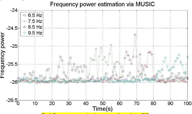
used in Table 3 were 6.5, 7.5, 8.5 and 9.5 Hz, respectively. 472

[image:8.612.111.518.53.281.2]

473

Table 1 Recognition rates under different conditions during the first session

474

in the synchronous mode[24] 475

Conditions * 1 2 3

A01 MUSIC 0.8571 0.9024 0.7073 CCA 0.7619 0.8293 0.6829

A03 MUSIC 0.8571 0.878 0.9268 CCA 0.7619 0.8293 0.9268

A05 MUSIC 0.8571 0.878 0.9268 CCA 0.7143 0.878 0.8537

A07 MUSIC 0.8571 0.8537 0.9268 CCA 0.8095 0.8293 0.9024

* Condition 1: data length=400, overlapping=0; number of channels=16; 476

Condition 2: data length=400, overlapping =50%; number of 477

channels=16; 478

channels=4. 480

481

In the first session of the asynchronous mode, subjects 482

looked at stimuli following predefined number sequences 483

‘1-2-3-4’, ‘1-3-2-4’ and ‘1-4-2-3’. Once a target was 484

recognized, subjects turned to look at another one 485

immediately. It is different from the experiments in the 486

synchronous mode, in which subjects looked at each 487

stimulus for a fixed period of time. 488

Table 2 Recognition rates under different conditions during the second

489

session in the synchronous mode[24] 490

Conditions* 1 2 3 4

A02 MUSIC 0.6607 0.5495 0.7928 0.8908 CCA 0.5 0.5135 0.6937 0.8829

A04

MUSIC 0.6429 0.5315 0.7838 0.8288

CCA 0.6429 0.6126 0.8108 0.8198

A06 MUSIC 0.7679 0.5856 0.8378 0.8829 CCA 0.6429 0.6667 0.8559 0.9099

A08 MUSIC 0.75 0.6937 0.9279 0.8649 CCA 0.75 0.5676 0.8288 0.8198 * Condition 1: data length=400, overlapping =0; number of 491

channels=16; 2 consecutive decisions (overlapping: 1) made one final target 492

choice; 493

choice; 496

choice; 499

choice. 502 503

Table 3 Recognition rates during the third session in the synchronous

504

mode[24] 505

Conditions MUSIC CCA

Far distance (8 cm), no use of covers 0.8025 0.8148

Far distance (8 cm), use of covers 0.8148 0.8025

Near distance (4 cm), no use of covers 0.7901 0.7531

[image:8.612.112.553.63.465.2] [image:8.612.67.254.359.492.2]

(9)

[image:9.612.110.504.59.250.2]

8 506

Fig. 7 Frequency power estimation in the asynchronous mode

507 508

Taking one number sequence ‘1-2-3-4’as an example, the 509

frequency power at four stimulus frequencies was illustrated 510

in Fig. 7. Subjects repeated looking at stimuli orderly three 511

times. The frequencies used were 6.5, 7, 7.5 and 8 Hz, 512

respectively. It means the frequency resolution was reduced 513

to 0.5 Hz, while the above experimental results were 514

obtained with frequency resolution of 1 Hz. As seen in Fig. 7, 515

frequencies with an interval of 0.5 Hz can be clearly 516

distinguished using the MUSIC method just like the 517

simulated data. 518

Five subjects participated in experiments. Each of them 519

finished looking at all stimuli corresponding to three number 520

sequences for three times. The experimental time 521

consumption for all subjects to complete different tasks is 522

listed in the following Table 4. 523

[image:9.612.36.279.461.692.2]

524

Table 4 Time consumption (seconds) during the first session in the

525

asynchronous experimental mode 526

Subjects Number sequences (repeating three times for each)

‘1-2-3-4’ ‘1-3-2-4’ ‘1-4-2-3’

Subject 1 57 57 57

Subject 2 58 59 63

Subject 3 57 51 55

Subject 4 57 58 61

Subject 5 60 62 59

527

Table 5 Recognition accuracy when subjects looked at stimuli randomly

528

Subjects Accuracy Total time (seconds)

Subject 1 1.0000 100

Subject 2 1.0000 103

Subject 3 0.9523 100

Subject 4 1.0000 101

Subject 5 0.9048 102

529

In the second session of the asynchronous mode, subjects 530

looked at whichever stimulus as they would like to for about 531

100 seconds. This situation is more like the real world 532

applications without external interference. The first session 533

was to estimate the time consumption time of target 534

recognition, while this one was to estimate the recognition 535

accuracy in the asynchronous mode as seen in Table 5. 536

3.3 SSVEP-based Virtual Keyboard 537

Fig. 4 illustrates the whole procedure of spelling the word 538

“BRAIN”. For five different subjects, the time consumption 539

of spelling “BRAIN” or “BCI TEST” was recorded as shown 540

in Table 6. 541

Table 6 shows the spelling speed for different subjects 542

were not the same even for the same word. As for “BRAIN”, 543

it takes 11.6 to 17 seconds to output a letter or a symbol. In 544

terms of “BCI TEST”, the average time is 15 to 15.88 545

seconds. Taking the word “BRAIN” as an example, the steps 546

of choosing these five letters starting from the keyboard 547

center are 2, 1, 2, 1 and 1, respectively. The total step is 7. 548

Considering the five “confirm” commands, 12 steps are 549

needed to spell the word “BRAIN”. It means each step takes 550

about 4.83 to 7.08 seconds. This time is longer than that of 551

the asynchronous mode experiments without device control. 552

It is partly because subjects need time to choose which the 553

next target is when spelling a specific word. 554

555

Table 6 Time consumption for different subjects of spelling different words

556

Subjects Words Time (Seconds)

Subject 1 BRAIN 58

Subject 2 BRAIN 68

Subject 3 BCI TEST 120

Subject 4 BCI TEST 127

Subject 5 BRAIN 85

4 DISCUSSION 557

4.1 Enhancement of Frequency Resolution 558

For stimulated data, the MUSIC method was used to 559

estimate the power at two nearby frequencies. As for FFT, 560

power values can be computed only at points where the 561

(10)

such as, 0, 0.5, 1, 1.5 Hz and so on. In Fig. 5(b), it is obvious 563

that two maxima appear at around 5.3 and 5.8 Hz, which are 564

the real harmonic components of the stimulated data. That 565

means the MUSIC method can achieve high frequency 566

resolution. In addition, MUSIC decomposes data into signal 567

subspace and noise subspace. The noise can be removed to 568

some extent when estimating the power spectrum. 569

4.2 One-target Recognition 570

For the real SSVEP signals, we compared the 571

experimental results of MUSIC and another typically used 572

method CCA. As shown in Tables 1-3, the MUSIC method 573

achieved higher recognition accuracy in most cases. 574

Exceptions existed, as the numbers in red color in these 575

tables illustrated that CCA performed better than MUSIC 576

sometimes. 577

In Table 1, one subject looked at only one stimulus for 40 578

seconds. All segmented data length was 2 seconds. The 579

accuracy was better when 50% data overlapping was used 580

for 16-channel SSVEP signals. Also, the results showed that 581

4-channel (P3, P4, O1 and O2) signals could be utilized for 582

detecting the target stimulus except dataset A1. This is 583

because not all frequencies evoke strong SSVEPs when 584

applied to different individuals. It is proved that more 585

channels do not definitely produce better results, because 586

SSVEP signals are not evenly distributed on the brain 587

surface. Some channels might contain more noise rather 588

than SSVEP related signals. In addition, reducing the 589

number of channels shortens the preparation time before 590

experiments, which is important for implementing a real BCI 591

system. 592

4.3 Idle State Detection 593

[image:10.612.47.286.444.524.2]

594

Fig. 8 A dwell time used for final decisions

595 596

The frequency with the maximum power value was 597

recognized as the target one in Table 1. However, in the idle 598

state, when subjects didn’t focus on any stimulus, this

599

method could cause false positives. Idle state detection 600

becomes another key issue. There are two common ways to 601

solve this problem. A dwell time or a threshold can be 602

employed for idle state detection. The accuracy in Table 2 603

was calculated by using a dwell time. A same target was 604

recognized for several consecutive times, and then a final 605

decision was made as seen in Fig. 8. Fig. 8 shows that three 606

consecutive decisions make a final decision, which means if 607

three consecutive one-time decisions are identical, and then a 608

final decision is made to confirm a target. The overlapping 609

percentage is 2/3 in this example. That means there is a 610

‘decision window’ moving along the time axis. It can be seen

611

in Table 2 that under condition 4, where the data length was 612

400 points with 50% overlapping and the number of 613

channels was 4, better performance was achieved than other 614

conditions. 615

For comparison, the threshold method was also employed. 616

The threshold was obtained from training data. For each 617

stimulus frequency, a period time of data in the work state 618

and the idle state was acquired. The threshold was adjusted 619

to maximize the total recognition rate, which was defined as 620

value of the sum of true positives and true negatives divided 621

by the total training number. 622

As seen in Table 7, the idle state could be better detected 623

by using a threshold. If the threshold and the dwell time were 624

used together, the recognition accuracy can be even up to 625

100%, such as dataset A06. It is noticed that using a 626

threshold can achieve better results, but it is more time 627

consuming compared with using a dwell time. Preparation 628

time is needed to acquire training data for all stimulus 629

frequencies. Recognition accuracy was higher than 83% 630

when using a dwell time in experiments. And there is no 631

extra time needed in advance. That is an advantage of using a 632

dwell time. However, a longer dwell time leads to delay of 633

recognition. In real applications, the choice of the dwell time 634

should be considered based on requirements of the detection 635

speed and the detection accuracy. 636

637

Table 7 Recognition rates with a threshold during the second session

638

in the synchronous mode 639

Conditions* A02 A04 A06 A08

1 0.8468 0.8468 0.8378 0.8739

2 0.8559 0.7658 0.8739 0.8739

3 0.9640 0.9820 1.0000 0.9820 *Condition 1: data length=400, overlapping =50%; number of 640

choice; 642

channels=4; a threshold made one final target choice; 644

channels=4; a threshold and 2 consecutive decisions (overlapping: 1) made 646

one final target choice. 647

4.4 Multi-target Recognition 648

649

Table 8 Recognition rates under different conditions during all sessions in

650

the synchronous mode[24] 651

A01 MUSIC 0.7869 A06 MUSIC 0.8378

CCA 0.7705 CCA 0.7748

A02 MUSIC 0.8468 A07 MUSIC 0.9180

CCA 0.8649 CCA 0.8852

A03 MUSIC 0.7705 A08 MUSIC 0.8739

CCA 0.7377 CCA 0.8198

A04 MUSIC 0.8468 B01 MUSIC 0.716

CCA 0.8649 CCA 0.7284

A05

MUSIC 0.7869

B02

MUSIC 0.6914

CCA 0.6885 CCA 0.6914

652

Table 3 reflects the recognition accuracy when subjects 653

[image:10.612.316.569.551.701.2]

(11)

10 flickering. The influence of stimulation design on 655

recognition results was tested in experiments. If two 656

neighboring stimuli were too close, it was not easy for 657

subjects to focus on one stimulus. This explained the poor 658

results. Through experiments, a distance of 4 cm seemed 659

reasonable. The distance made the stimulation panel not too 660

big, and the mutual influence of nearby stimuli could be 661

reduced. Also, a layer of thin paper was covered on the 662

stimuli, which made the light more centralized. Recognition 663

rates shown in Table 3 proved that it did improve the 664

recognition results. 665

The idle state data and the work state data were analyzed 666

alone with or without the use of a dwell time as discussed 667

above. In real applications, all data should be processed 668

under the same condition. Table 8 shows the recognition 669

results of one subject during all three sessions. Three 670

consecutive decisions with 2/3 overlapping made a final 671

target choice. It is shown in Table 8 that the recognition rates 672

in the work state were reduced compared with the situation 673

when no dwell time was used. Subjects might have difficulty 674

in keeping focusing on one stimulus for 40 seconds. This 675

affected the overall recognition accuracy. For the third 676

session, the results became even worse. This is mainly 677

caused by the transition from looking at one stimulus to 678

looking at another, as seen in Fig. 9 showing the stimulus 679

frequency power values of data B02 in Table 8. It took time 680

for subjects to get used to another stimulus. The response 681

time made the results worse. In addition, 80 seconds was 682

quite a long time for subjects to keep focused during this 683

session. The results could be affected if subjects’ attention 684

was distracted. 685

[image:11.612.120.496.242.465.2]

686

Fig. 9 Frequency power estimation corresponding to dataset B02

687 688

4.5 Asynchronous Mode Target Recognition 689

In the asynchronous mode, from both Fig. 7 and Table 4, it 690

can be estimated that it took about 5 seconds to finish 691

one-target recognition. But the consumption time is different 692

for different subjects or sequences. Actually the original data 693

were processed every one second, but subjects couldn’t 694

move eyes from one stimulus to another instantly. The 695

response time existed inevitably when subjects were 696

informed to look at the next stimulus. At most times, one 697

response potential was evoked following a former potential 698

quickly. However, for each potential, it lasted for a period of 699

time. Also, a dwell time caused the delay of one final 700

decision, which made the whole procedure longer. 701

In the second session, the accuracy when subjects looked 702

at stimuli as they wanted for about 100 seconds was tested. 703

The performance was quite good as seen in Table 5. Three of 704

them achieved accuracy of 100%. For this experiment, not 705

only the target stimulus should be recognized, but also the 706

idle state had to be detected. For all experiments in the 707

asynchronous mode, a dwell time was used to reduce false 708

positives. In addition, the idle state detection was conducted 709

in this asynchronous mode. All stimuli were flickering and 710

the subject looked other places rather than the stimulation 711

panel for 100 seconds. However, in the previous 712

synchronous mode, only one of the stimuli was on and the 713

subject looked at other stimuli areas even they were not 714

flickering. This test in the asynchronous mode means 715

subjects are completely in an idle state without any external 716

interference. The recognition accuracy for this experiment is 717

shown in the following Table 9. 718

[image:11.612.346.561.612.710.2]

719

Table 9 Idle state detection in the asynchronous mode

720

Subjects Accuracy Total time (seconds)

Subject 1 0.9303 100

Subject 2 0.9055 100

Subject 3 0.9950 100

Subject 4 0.8905 100

Subject 5 0.9876 100

721

(12)

this experiment than that in the synchronous mode for idle 723

state detection. The subjects kept in an idle state for a period 724

of 100 seconds, and the detection accuracy for Subject 3 was 725

even up to 99.50%, which is a satisfactory result. For in this 726

experiment, although all stimuli were flickering, the subject 727

looked at other areas rather than the stimuli. While for the 728

previous one, the flickering stimulus had influence when 729

subjects looked at other stimuli areas. Also, no predefined 730

time duration was set in the asynchronous mode. All these 731

contributed to good results. 732

4.6 Number of Eigenvectors Constituting the Signal 733

Subspace 734

735

Table 10 Recognition rates when p is a constant or adjustable

736

Data p: constant p: adjustable

A01 0.5372 0.5372

A02 0.9095 0.9457

A03 0.6529 0.7438

A04 0.9231 0.9819

A05 0.6033 0.6529

A06 0.9548 0.9593

A07 0.8430 0.8512

A08 0.9186 0.9276

737

It was mentioned that a segmentation ratio was proposed 738

to confirm the number of eigenvectors to be used for 739

constituting the signal subspace of the MUSIC method in our 740

research. This value can be set to a constant, too. Let

p

741

represent this value. We did experiments to compare the 742

recognition results as shown in Table 10 by using the 743

constant method and the proposed method. 744

Table 10 reflects that the proposed method produced 745

better results. It is more flexible than the constant method. 746

However, the segmentation ratio is set to be 0.01 in our 747

research. This ratio was obtained after conducting some 748

previous data analysis, too. 749

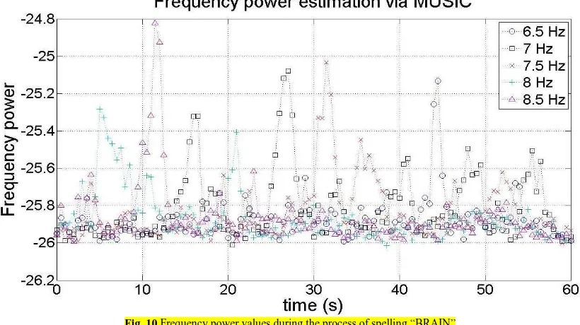
4.7 Control of a Virtual Keyboard 750

Fig. 10 illustrates the power values corresponding to five 751

stimuli. The five frequencies are 6.5, 7, 7.5, 8 and 8.5 Hz, 752

which are mapped to five numbers 1, 2, 3, 4 and 5. The 753

numbers are used to represent five commands: up, confirm, 754

left, down and right. 755

As seen in Fig. 10, the frequency corresponding to the 756

maximum power value is different during the spelling 757

process. The number sequence is “4-5-2-4-2-3-3-2-1-2-3-2” 758

when mapping the frequencies to numbers. This sequence is 759

translated to commands

760

“up-right-confirm-down-confirm-left-left-confirm-up-confir 761

m-left-confirm”. According to these commands, five letters 762

B, R, A, I and N are selected. It takes about 60 seconds to 763

finish the whole procedure, which means each step 764

consumes about 5 seconds. It is noticed that a control 765

strategy was used during the spelling procedure. Only if one 766

recognition number (corresponding to one frequency target) 767

lasts for a certain period of time, is a control command 768

confirmed. This explains the recognition time is longer than 769

that of the asynchronous mode experiments without device 770

control, too. If the commands change too quickly, the cursor 771

moves quickly. It is hard for subjects to focus on one letter or 772

symbol. Also, the subjects need time to decide the move path 773

of the cursor. This is why the control strategy is necessary. 774

775

[image:12.612.75.244.220.360.2]

776

Fig. 10 Frequency power values during the process of spelling “BRAIN” 777

778

5 CONCLUSIONS 779

SSVEP-based BCI systems have great potential in real 780

world applications, and the signal processing algorithm is of 781

great importance. In this paper, a MUSIC-based method was 782

[image:12.612.101.511.453.683.2]

(13)

12 segmentation ratio for determining the number of 784

eigenvectors constituting the signal subspace was suggested. 785

The experimental results with simulated data proved that 786

this method could provide high frequency resolution. Also, 787

the multi-channel(dimensional) signals have the anti-noise 788

ability, so the power spectrum estimation is more accurate. 789

The method was verified with real SSVEP signals 790

acquired in an unshielded environment. The original data 791

were segmented into 2-second epochs with a sampling 792

frequency of 200 Hz. Four channels were enough for feature 793

extraction. The basic idea was to compute the frequency 794

power at stimulus frequencies. Then the frequency with the 795

maximum power value was recognized as the target one. The 796

results showed targets could be well recognized either one 797

stimulus was on or all stimuli were on, compared with a 798

typical multi-channel signal processing method CCA. It was 799

feasible to detect the idle state using a dwell time in our 800

experiments. A disadvantage of this method is that it caused 801

time delay for each decision. An alternative way is to use a 802

threshold, which was obtained with training data. In our 803

research, the threshold was gradually adjusted to maximize 804

the overall recognition accuracy of the training data. Though 805

it didn’t cause recognition delay, the preliminary time was 806

longer. 807

Finally, the proposed method was implemented in a real 808

time application of keyboard control. Different subjects 809

could use the virtual keyboard successfully. 810

Future work includes improving the algorithm to 811

recognize the target within less time and with higher 812

accuracy. Other factors like design of the stimuli, the 813

subjects comfort, all should be taken into account to develop 814

practical applications for disabled people. 815

ACKNOWLEDGEMENTS 816

This work was supported by the National Science 817

Foundation (Grant No. 51475342). The authors would like to 818

thank all subjects for their participating in the experiments. 819

REFERENCES 820

1. Wolpaw JR, Birbaumer N, Heetderks WJ, McFarland DJ, 821

Peckham PH, Schalk G, Donchin E, Quatrano LA, 822

Robinson CJ, Vaughan TM (2000) Brain-computer 823

interface technology: A review of the first international 824

meeting. IEEE Trans. Rehabil. Eng. 8 (2):164-173 825

2. Mason SG, Birch GE (2003) A general framework for 826

brain-computer interface design. IEEE Trans. Neural 827

Syst. Rehabil. Eng. 11 (1):70-85 828

3. Wang Y WR, Gao X (2006) A practical VEP-based 829

brain-computer interface. IEEE Trans. Neural Syst. 830

Rehabil. Eng. 14 (2):234-240 831

4. Picton T (1990) Human brain electrophysiology: evoked 832

potentials and evoked magnetic fields in science and 833

medicine. J. Clin. Neurophysiol. 7:450-451 834

5. Bin GY, Gao XR, Yan Z, Hong B, Gao SK (2009) An 835

online multi-channel SSVEP-based brain-computer 836

interface using a canonical correlation analysis method. 837

J. Neural Eng. 6 (4):1-6(046002) 838

6. Liu Q, Chen K, Ai Q, Xie SQ (2014) Review: Recent 839

Development of Signal Processing Algorithms for 840

SSVEP-based Brain Computer Interfaces. J. Med. Biol. 841

Eng. 34 (4):299-309 842

7. Muller-Putz GR, Pfurtscheller G (2008) Control of an 843

electrical prosthesis with an SSVEP-based BCI. IEEE 844

Trans. Biomed. Eng. 55 (1):361-364 845

8. Bian Y, Li HW, Zhao L, Yang GH, Geng LQ (2011) 846

Research on steady state visual evoked potentials based 847

on wavelet packet technology for brain-computer 848

interface. Proc. Eng. 15:2629-2633 849

9. Zhang Z, Li X, Deng Z (2010) A CWT-based SSVEP 850

classification method for brain-computer interface 851

system. In: Internation Conference on Intelligent Control 852

and Information Processing, pp 43-48 853

10.Yan B, Li Z, Li H, Yang G, Shen H (2010) Research on 854

brain-computer interface technology based on steady 855

state visual evoked potentials. In: 4th_{International} 856

Conference on Bioinformatics and Biomedical 857

Engineering, pp 1-4 858

11.Wu CH, Chang HC, Lee PL, Li KS, Sie JJ, Sun CW, 859

Yang CY, Li PH, Deng HT, Shyu KK (2011) Frequency 860

recognition in an SSVEP-based brain computer interface 861

using empirical mode decomposition and refined 862

generalized zero-crossing. J. Neurosci. Methods 196 863

(1):170-181 864

12.Wu CH, Chang HC, Lee PL (2009) Instantaneous 865

gaze-target detection by empirical mode decomposition: 866

application to brain computer interface. In: World 867

Congress on Medical Physics and Biomedical 868

13. Friman O, Luth T, Volosyak I, Graser A (2007) Spelling 870

with steady-state visual evoked potentials. In: 3rd 871

International IEEE/EMBS Conference on Neural 872

14. Volosyak I (2011) SSVEP-based Bremen-BCI interface - 874

boosting information transfer rates. J. Neural Eng. 8 875

(3):1-11(036020) 876

15. Volosyak I, Malechka T, Valbuena D, Graser A (2010) A 877

novel calibration method for SSVEP based 878

brain-computer interfaces. In: 18th_{European Signal Proc.} 879

Conf., pp 939-943 880

16.Cecotti H (2010) A self-paced and calibration-less 881

SSVEP-based brain-computer interface speller. IEEE 882

Trans. Neural Syst. Rehabil. Eng. 18 (2):127-133 883

17.Zhang ZM, Deng ZD (2012) A kernel canonical 884

correlation analysis based idle-state detection method for 885

SSVEP-based brain-computer interfaces. In: 2nd 886

International Conference on Material and Manufacturing 887

Technology, pp 634-640 888

18. Lin ZL, Zhang CS, Wu W, Gao XR (2006) Frequency 889

recognition based on canonical correlation analysis for 890

SSVEP-based BCIs. IEEE Trans. Biomed. Eng. 53 891

(12):2610-2614 892

19. Hakvoort G, Reuderink B, Obbink M (2011) Comparison 893

of PSDA and CCA detection methods in a SSVEP-based 894

BCI-system. Centre for Telematics and Information 895

Technology, University of Twente. 896

http://eprints.eemcs.utwente.nl/19680/01/Comparison_o 897

(14)

ased_BCI-system.pdf 899

20. Schmidt RO (1986) Multiple emitter location and signal 900

parameter estimation. IEEE Trans. Antennas Propag. 34 901

(3):276-280 902

21. Swami A, Mendel JM, Nikias CL (1998) Higher-order 903

Spectral Analysis Toolbox: for Use with MATLAB: 904

User's Guide. Mathworks, Incorporated 905

22. Wang Yongliang CH, Peng Yingning, Wan Qun (2004) 906

Theories and algorithms of spatial spectrum estimation. 907

Press of Tsinghua University 908

23.Hardoon D R SS, Shawe-Taylor (2004) Canonical 909

correlation analysis: An overview with application to 910

learning methods. Neural Comput. 16 (12):2639-2664 911

24. Chen K, Liu Q, Ai QS (2014) Multi-channel SSVEP 912

pattern recognition based on MUSIC. In: 4th 913

International Conference on Intelligent Structure and 914

Vibration Control, pp 84-88 915