Online Detection of Particle Agglomeration during Solution Crystallization by Microscopic Double-View Image Analysis

White Rose Research Online URL for this paper: http://eprints.whiterose.ac.uk/122286/

Version: Accepted Version

Article:

Huo, Y, Liu, T, Wang, XZ et al. (2 more authors) (2017) Online Detection of Particle

Agglomeration during Solution Crystallization by Microscopic Double-View Image Analysis. Industrial & Engineering Chemistry Research, 56 (39). pp. 11257-11269. ISSN 0888-5885 https://doi.org/10.1021/acs.iecr.7b02439

© 2017 American Chemical Society. This document is the Accepted Manuscript version of a Published Work that appeared in final form in Industrial and Engineering Chemistry Research, copyright © American Chemical Society after peer review and technical editing by the publisher. To access the final edited and published work see

https://doi.org/10.1021/acs.iecr.7b02439

[email protected] https://eprints.whiterose.ac.uk/

Reuse

Items deposited in White Rose Research Online are protected by copyright, with all rights reserved unless indicated otherwise. They may be downloaded and/or printed for private study, or other acts as permitted by national copyright laws. The publisher or other rights holders may allow further reproduction and re-use of the full text version. This is indicated by the licence information on the White Rose Research Online record for the item.

Takedown

If you consider content in White Rose Research Online to be in breach of UK law, please notify us by

On-line detection of particle agglomeration during solution crystallization

by microscopic double-view image analysis

Yan Huo a, Tao Liu a,*, Xue Z. Wang b, c, Cai Y. Ma b, Xiongwei Ni d

a

Institute of Advanced Control Technology, Dalian University of Technology, Dalian, China

b _{School of Chemical and Process Engineering, University of Leeds, Leeds, LS2 9JT, UK} c

School of Chemistry and Chemical Engineering, South China University of Technology, Guangzhou, China

d _{School of Engineering and Physical Science, Heriot-Watt University, Edinburgh, UK}

* Corresponding author. Tel: + 86-411-84706465; Fax: + 86-411-84706706; E-mail: [email protected]

Abstract: To detect the particle agglomeration degree for assessing crystal growth quality during a

crystallization process, an in-situ image analysis method is proposed based on a microscopic

double-view imaging system. Firstly, a fast image preprocessing approach is adopted for segmenting raw

images taken simultaneously from two cameras installed at different angles, to reduce the influence

from uneven illumination background and solution turbulence. By defining an index of the inner

distance based curvature for different particle shapes, a preliminary sieving algorithm is then used to

identify candidate agglomerates. By introducing two texture descriptors for pattern recognition, a

feature matching algorithm is subsequently developed to recognize pseudo agglomerates in each pair

of the double-view images. Finally, a fast algorithm is proposed to count the number of recognized

particles in these agglomerates, besides the unagglomerated particles. Experimental results from the

potassium dihydrogen phosphate (KDP) crystallization process demonstrate good accuracy for

recognizing pseudo agglomeration and counting the primary particles in these agglomerates by using

the proposed method.

Keywords: particle agglomeration; pseudo agglomerate; double-view image analysis; feature

1. Introduction

On-line imaging systems have been increasingly applied to monitor industrial crystallization

processes at the micro-scale in the last two decades 1-5, offering on-line observation of the crystal

shapes related to crystal morphology and growth rate. By using high-speed microscopic camera sensors,

e.g., the particle vision and measurement (PVM) instrument 6, 7 and the non-invasive imaging system8,

a small number of image analysis methods were explored in the recent references 9-13 _{for on-line}

measurement of crystal size distribution (CSD) during a crystallization process. However, the influence

from uneven illumination background and solution turbulence on in-situ imaging in a continuously

stirred crystallizer was not fully considered in literature. Such influence may provoke significant

misestimate of crystal morphology or CSD by using the existing image processing methods, as studied

in the recent paper 14. Development of advanced in-situ image analysis methods has been eagerly

appealed for on-line monitoring, control and optimization of various crystallization processes 3, 15_.

Particle agglomeration is commonly associated with crystallization processes due to particle

collisions in the stirred crystal suspension, which has a considerable impact on the crystal properties

such as the dissolution rate, precipitation, filtration, drying, milling and grinding. It is one of the main

tasks to control the agglomeration degree for industrial crystallization processes 16_{. Image-based}

detection of particle agglomeration has therefore been increasingly studied for on-line control and

optimization. In the early study 17_{, detecting agglomerates from crystal images was performed off-line}

by using a statistical principal component analysis (PCA) approach. Ferreira et al. 18 presented an

automatic classification tree to distinguish different classes of sucrose crystals and the agglomeration

degree. Terdenge et al. 19 developed an image processing method based on a discriminant factorial

analysis to evaluate the agglomeration degree of crystalline products. Ochsenbein et al. 20 _{presented a}

machine learning method to identify the agglomeration of needle-like crystals together with the

primary particles involved in these agglomerates. Borchert et al. 21 _{developed an image-based}

identification method for monitoring the growth rate of crystals such as the potassium dihydrogen

phosphate (KDP) that is a typical case of morphology evolution for multi-dimensional CSD

measurement and verification.

crystallization process, due to overlapped particles which have different distances to the camera lens.

These pseudo agglomerates inevitably affect image-based measurement accuracy of CSD and the true

agglomeration degree. To solve the problem, it was suggested to adopt double-view images for

recognizing pseudo agglomerates 20, but how to realize exact feature matching for overlapped particles

in each pair of view images remains open. Regarding feature matching between the

double-view images taken for the same object, a widely recognized matching algorithm is the scale invariant

feature transform (SIFT) 22, where a 128-dimensional descriptor was established from a

three-dimensional (3D) histogram of gradient locations and orientations, while using a weighting function

of the gradient magnitude for each location bin to ensure efficient matching. An alternative interest

point descriptor was proposed to construct another matching algorithm named ASIFT 23 _{which may}

procure improved matching effect in some cases, but at the cost of larger computation effort. To

alleviate the computation load of SIFT, Bay et al. 24 _{developed a fast algorithm so called speeded up}

robust features (SURF), which computed the Haar wavelet responses via the integral images instead

of the gradient information. By comparison, Rublee et al. 25 _{proposed a faster matching algorithm}

called ORB by using the binary descriptors, which demonstrated good robustness to

rotational variation and measurement noise.

Note that particles in microscopic double-view images taken from a crystallization process

typically have high similarity in the feature properties, thus bringing difficulty to feature distinction by

using the aforementioned matching methods. To efficiently address the problem of feature similarity

among these images, texture statistical analysis was adopted as an alternative descriptor for image

matching in literature. By defining the local binary pattern (LBP) 26, both the statistical and structural

characteristics of image texture were used for double-view image matching. A few modified LBP

descriptors have been developed in the reference 27 for better texture classification and image

recognition. To enhance the performance of LBP, a completed LBP modeling was developed for texture

classification 28, which extracted the local gray levels and magnitude features among these images,

respectively. The approach was further extended by defining the LBP variance (LBPV) to characterize

the local contrast information in a one-dimensional LBP histogram for matching 29. By comparison,

distributions to represent consistent patterns. However, it remains open for implementing the above

methods for on-line recognition of particle agglomeration in engineering applications, in particular for

poor imaging conditions during a crystallization process.

In this paper, an in-situ double-view image analysis method is proposed for recognizing pseudo

particle agglomeration during a crystallization process, by establishing a double-view image matching

algorithm based on feature analysis. Firstly, an image preprocessing strategy is used to reduce the

influence from uneven illumination background, solution turbulence, and measurement noise. Then a

preliminary sieving algorithm is given to screen out candidate agglomerates for mitigating the

subsequent computation load, by defining an index to distinguish candidate agglomerates from all

particles. By introducing two new texture descriptors for pattern recognition, a feature matching

algorithm is proposed to recognize pseudo agglomeration. The number of primary particles involved

in these agglomerates is counted by establishing a fast algorithm. The rock-like crystals of KDP as

studied in the references 21, 31 for image analysis are used for experimental tests to demonstrate the

effectiveness of the proposed method for on-line detection.

For clarity, the paper is organized as follows. Section 2 briefly states the problem of detecting

particle agglomeration. In Section 3, an image preprocessing method is presented to alleviate the

influence from in-situ imaging conditions during the process operation. In Section 4, a preliminary

sieving algorithm is given to screen out candidate agglomerates. A feature matching algorithm is

proposed to recognize pseudo agglomerates in Section 5, along with an illustration on the advantage

of the proposed texture descriptors compared to the existing image feature matching algorithms.

Section 6 presents a fast algorithm to count the primary particles involved in the agglomerates.

Experimental results are shown in Section 7 to demonstrate the effectiveness and advantage of the

proposed method. Some conclusions are drawn in the last Section 8.

2. Problem of detecting particle agglomerates during crystallization

2.1 Double-view imaging system for monitoring a crystallizer

A non-invasive microscopic imaging system for monitoring industrial crystallization processes

high-speed cameras made by Hainan Six Sigma Intelligent Systems Ltd was used to capture crystal

images synchronously during the cooling crystallization process. The two cameras (UI-2280SE-C-HQ)

with USB Video Class standard were made by IDS Imaging Development Systems GmbH, including

two micro telescope lenses. The angle between these camera optic axes was set about 18 degrees to

capture double-view images with two LED lights.

As shown in Figure 1, the crystallizer was composed of a 4-liter glass vessel, a 4-paddle agitator

(PTFE), a thermostatic circulator (Julabo-CF41), and a temperature probe (PT100). Chemical

compound used for the experiments was KDP (KH2PO4) with distilled water (H2O) as solvent. The

crystal suspension was monitored by the non-invasive microscopic double-view imaging system

installed outside the vessel.

2.2 In-situ detection of particle agglomeration

In-situ image monitoring of particles in the suspension brings much more complexity compared

to off-line image analysis of particles by using an optic microscopy. The major challenge lies in the

fact that particle motion and solution turbulence in a stirred crystallizer provoke image blurring and

additional noise. Secondly, the uneven light effect and time-varying hydrodynamics in the crystallizer

interferes with the uniformity and intensity of the image background. In addition, there may be

different gray scales between double-view images captured for the same particles, due to unequal

distances from two camera lenses to the same particles. A typical scenario of double-view images is

shown in Figure 2 by using the above imaging system.

It can be seen from the left view of Figure 2 that there possibly exists particle agglomeration. In

fact, it can be verified from the right view of Figure 2 that the visual agglomerates were caused by

particles overlapping in the left view. The phenomenon has been recognized as pseudo agglomeration

in the literature. Herein the overlapped particles are defined by pseudo agglomerate for analysis. It is

obvious that a single-view image, subject to lots of pseudo agglomerates, could mislead counting the

crystal number and size, and thus affects on-line control and optimization of the crystal growth and

product quality. Therefore, the recognition of pseudo agglomeration should be envisaged for on-line

literature, since the emergence of in-situ microscopic imaging technology for monitoring

crystallization processes in the recent years 3, 8_.

To cope with the above problems, an in-situ image analysis method is proposed in this paper for

detecting particle agglomeration during a crystallization process. The key idea is to recognize pseudo

agglomerates by particle sieving and feature matching between double-view images. Correspondingly,

the number of agglomerated particles can be efficiently counted. The agglomeration degree is

evaluated by using the following specification 32,

A Ap p

100% N

P N

  (1)

where NAp is the number of primary particles involved in the agglomerates, Np is the total number

of valid particles counted in the image. Note that the primary particles means the recognized particles

in these agglomerates, which originate from unagglomerated particles during the crystallization

process. Correspondingly, the valid particles include these primary particles and unagglomerated

particles detected in the captured image.

A flowchart of the proposed double-view image analysis method is shown in Figure 3.It can be

seen that there are four steps for on-line implementation, including image preprocessing, preliminary

sieving, feature matching, and particle counting, as detailed in the following sections, respectively.

3. Image preprocessing

3.1 Image reduction

For using a microscopic imaging system, the size of an image depends on the system resolution

and the magnification of camera lens. A larger image size corresponds to a longer time delay for

on-line analysis. An efficient image reduction method is therefore adopted to shrink the size of a captured

image while maintaining fundamental image features to facilitate on-line analysis. Considering that

the method has the advantage of high reduction ratio and good denoising ability, a two-dimensional

discrete wavelet transform algorithm with the bi-orthogonal wavelet function 33 _{is constructed for a}

captured image denoted by I x y with a size of M N( , )  . Denoting by m the row, by n the

wavelet transform for I x y is defined as ( , ) , , 1 1 1 ( , , ) ( , ) ( , ) M N

j m n

x y

A j m n I x y x y

MN   





where

/2

, , ( , ) 2 (2 , 2 )

j j j

j m n x y x m y m

     ₍₃₎

Then the low frequency component A j m n( , , ) is used to approximate the original image I x y( , ).

As a result, a reduction image f x y( , ) is constructed from the low frequency component.

3.2 Image segmentation

To alleviate the influence from uneven image background, morphology processing is considered

as an efficient approach based on the crystal shape characteristics. The uneven background is extracted

by using an opening operation algorithm with the structuring element 34.

To properly parameterize the structuring element, a watershed transform algorithm 33 is used for

computation. The watershed transform algorithm classifies catchment basins and watershed ridge lines

in an image by treating it as a surface where light and dark pixels correspond to high and low values,

respectively. The averaged distance between the watershed ridge lines is taken as a parameter of the

structuring element. Then the uneven background is extracted by using the above algorithm.

Subsequently, the raw image is subtracted by the above uneven background. The segmentation

threshold t* _{is computed by using the Otsu thresholding function} 33 as





* 2

arg max ( )

t

t   t ₍₄₎

where 2( )t is the variance between two gray level classes with a threshold value of t[1, ]L and

L is the maximum gray level.

Finally, the segmented image is obtained by

* *

0, ( , )

( , )

1, ( , )

f x y t

q x y

f x y t

 

  



 (5)

After the segmentation, morphological region filling is performed to fill up all the holes inside

the segmented image q x y( , ), such that the resulting image only remains all the particle regions while

4. Preliminary sieving

This step is to screen out candidate agglomerates by using the particle shape features from the

segmented double-view images, in order to save computation time for specifically recognizing pseudo

agglomerates among these candidate agglomerates, while counting the number of valid particles in

these images.

In fact, it remains open to describe the shape feature of particle agglomeration, though a few

features describing particle shapes were explored in the literature 8, 20_{. In this work, the inner distance}

descriptor recently proposed in the reference 14 _{is further extended to describe the agglomeration}

feature so as to sieve out the candidate agglomerates efficiently. The coordinates of particle boundary

are denoted by ( ,x y , _{n n}) n1, 2, ,N, and the centroid coordinate ( ,x y is denoted by c c)

1 c 0 1 c 0 1 1 N n n N n n x x N y y N      _     





The distances from the particle centroid to its boundary points are defined as

2 2

c c

( ) ( )

n n n

d  x x  y y (7)

A deviation distance is defined by

n dn d

   (8)

where d is the mean value of d . n

The curvature of _n is computed by

2 3/2 ''

(1 ' )

n n n c     (9)

An index of the inner distance based curvature (IDC) is therefore proposed as

1 IDC N n n c N 





For illustration, Figure 4shows a few simplified round-like shapes of an unagglomerated particle

and three agglomerates involved with two, three, and four particles, respectively. It is found that the

candidate agglomerates. Note that for rod-like and needle-like particle shapes, the corresponding IDC

indices may be similar to those of the involved agglomerates, due to a relatively large length-width

ratio of such a particle or agglomerate. Additional shape features, e.g., the specific elongation ratios

and perimeters of different crystals, Fourier descriptors, and geometric moments as studied in the

reference 14_{, may be adopted to further recognize candidate agglomerates.}

Based on collecting typical shapes of individual particles and agglomerates in a crystallization

process, the corresponding IDC indices are constructed as a training set for preliminary sieving. By

classifying all the IDC indices into two groups, one for candidate agglomerates and the other for

unagglomerated particles, a linear classification algorithm is established below.

Denote by a and ₁ a for the IDC index groups of candidate agglomerates and unagglomerated ₂

particles, respectively. The central value u of _{i a (i} i1, 2) is computed by

2

arg min || || , 1, 2

i

i i i

u

u 



The threshold t for classification is determined by ₀

1 2

0 2

u u

t   (12)

To determine whether a segmented image region with an IDC index of b belongs to an

agglomerate, a classification rule is proposed as follows:

0 0

CA1, ;

CA2, .

if b t b

if b t

 

 _

 (13)

where CA1 denotes the candidate agglomerate set and CA2 indicates the unagglomerated particle

set.

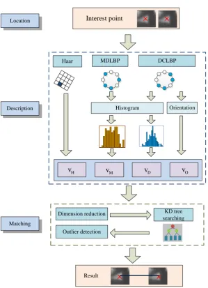
5. Feature matching

To further recognize the pseudo agglomerates from the candidate agglomerates, an enhanced

feature matching algorithm is proposed to procure accurate recognition, by establishing the image

interest point location and its feature descriptors as developed in the references 22-25. For clarity, Figure

5 shows the flowchart of the feature matching process. Note that the raw surfaces of particles in the

segmented double-view images are wholly stuffed within their contours before proceeding with the

5.1 Interest point location

The Hessian matrix studied in SURF 24 _{is used for detecting the interest point location. Given an}

image point Q x y( , ), the Hessian matrix H Q( , ) _{in X is defined as}

( , ) ( , )

( , )

( , ) ( , )

xx xy

xy yy

L Q L Q

H Q

L Q L Q

           

  (14)

where L Qxx( , ) is the convolution of the Gaussian second order derivative

2

2 g( )

x 



 with respect

to the image point Q, and so is for L Qxy( , ) and Lyy( , )Q  ,  is a parameter of the Gaussian

function g( ) , which denotes the image scale 22.

To simplify the above computation, box filters are used instead of the Gaussian second order

derivatives. Denoting D , xx Dyy and Dxy as the approximations of the Gaussian second order

derivatives for each image by using the box filters, respectively, an approximation determinant of the

Hessian matrix can be written as

2

Det( )H D D_{xx yy}(0.9D_xy) (15)

The scale space is described as an image pyramid, which is divided into 4 octaves, and each octave

includes 4 levels together with box filters of different window sizes denoted by L . By using the

integral image, the local maxima as a candidate interest point may be selected in a 3 3 3 

neighborhood in the scale space, such that the convolution computation could be accelerated 24.

For using the box filters, the parameters cannot be chosen arbitrarily. Following the guideline in

the reference 35, it is preferred to take

2 1 1.2 = 3 o L i L         (16)

where o{1, 2, 3, 4} is the octave index and i{1, 2, 3, 4} is the level index.

Moreover, a distance constraint is additionally imposed in the same scale  to avoid the interest

points over dense in a local area, because the density affects the matching efficiency. For example,

denoting  as the interest point set, a distance-constrained rule is defined for two interest points

1 1

( , )

X x y and X x y as ( ,2 2)

1 1 1 1 2 2

2 2 1 1 2 2

1 1 2 2

( , ) , < and ( , ) ( , ) 0

( , ) , < and ( , ) ( , ) 0

( , ) and ( , ) ,

X x y if Dis R x y R x y

X x y if Dis R x y R x y

X x y X x y if Dis

where Dis(x₁x₂)2(y₁y₂)2 , R x y( ,1 1) and R x y( ,2 2) denote gray levels, and  is a

distance threshold similar to the parameter of the structuring element in Section 3.2.

5.2 Feature descriptor

The Haar wavelet responses in SURF 24_{, which can be quickly computed via integral images, are}

used to construct a feature descriptor. Firstly, the dominant orientation of the Haar descriptor for the

interest point is computed by detecting the longest vector of the summed Gaussian weighted Haar

wavelet responses under a sliding sector window of  / 3.

To determine the descriptor, a square region is chosen around the interest point. The region is split

into smaller 4 4 square sub-regions. For each sub-region, the Haar wavelet response dx

perpendicular to the dominant orientation and the Haar wavelet response dy in the dominant

orientation are computed. Hence, a four-dimensional (4D) Haar descriptor,

(

 

 

each interest point, a Haar descriptor of 64 dimensions denoted by v is subsequently constructed H

after normalization.

To compensate for the deficiency of the above descriptor in dealing with image noise and uneven

illumination background, two texture descriptors are supplemented to enhance the matching accuracy

for double-view images with high feature similarity. Inspired by the LBP approach developed in the

references 27-30_{, a deviation compensated LBP (DCLBP) descriptor and a magnitude difference based}

LBP (MDLBP) descriptor are proposed to improve the accuracy of describing the interest region in the

presence of uneven illumination while mitigating the computation effort.

Denoting g as the gray value of the center pixel c ( , )i j in a local region, and gp

(p0,...,P1_{) as the gray values of equally spaced P pixels in a circle of radius R with respect}

to the center pixel ( , )i j , the location parameter g is defined as a

c , c c

1 a

c , c c

1

, 1 / (P 1) ( );

, 1 / (P 1) ( ).

P

P R p

p P

P R p

p

g std if g g g

g

g std if g g g





 _{   }

   

    







Thus, the DCLBP for G i j( , ) is obtained as

, a 1

( , ) ( )2

P

p

P R p

p

DCLBP i j s g g







where a a a 1, ; ( ) 0, . p p p

if g g T

s g g

if g g T

 



 _{ }

 

 (20)

where T is a practically specified difference threshold, e.g., -3 e .

Considering that the magnitude information is also important for local texture structure

description 28_{, we define the magnitude difference by}

c

| |

p p

m  g g . Note that the vector

0 1 1

[m m, ,...,m_P ] is less sensitive to uneven illumination, which is therefore transformed into the

binary pattern for analysis. Correspondingly, the MDLBP is obtained as

,

1

( , ) ( ) 2

P

p

P R p p

p

M D L B P i j s m m







where m is the averaged value for _p [m m0, 1,...,mP1], and

1, ( ) 0, p p p p p p

if m m T

s m m

if m m T

  



 _{ }

 

 (22)

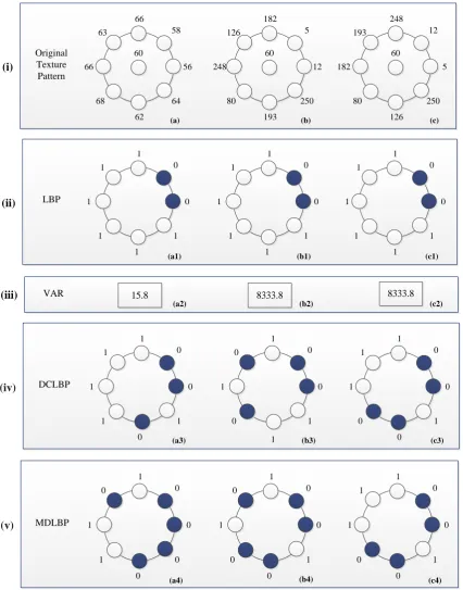
For illustration, a numerical example studied in the reference 30 _{is performed here to demonstrate}

the proposed texture recognition of image micro-structure. Figure 6 shows three texture patterns with

different features to classify and each of the patterns has the same center pixel with 8 neighbors. It is

obvious that LBP and the proposed DCLBP have different thresholds in terms of the same P 8. The

three patterns(a, b, c) are classified into the same pattern by using LBP, due to the oversimplified local

structure recognized by LBP. By introducing a complementary feature, called VAR, which could reflect

the local contrast of each pattern, The reference 26 _{proposed the combination of VAR and LBP for}

recognition, as shown in Figure 6 (ii) and (iii). It can be seen that the patterns (a) and (b) can be

distinguished but the patterns (b) and (c) are still regarded as the same texture, due to neglecting the

differences between the center and each neighbor. In contrast, both of the proposed DCLBP and

MDLBP have effectively recognized different binary patterns for these three texture patterns, as shown

in Figure 6 (iv) and (v), owing to further detailed description of local texture feature in the interest

Moreover, taking into account the rotation invariance of LBP 26_{, we denote} Ri

, ( , ) P R

DCLBP i j and

Ri , ( , ) P R

MDLBP i j as the rotation invariants of DCLBP and MDLBP, respectively. Distribution

histograms of the DCLBP and MDLBP values are taken as two dimensions in the feature descriptor.

The property of the histogram may facilitate analyzing the statistical region characteristics and

reducing the pattern dimension 29_{. Take the DCLBP as an example, in the interest region N N} _for

the interest point, the DCLBP value of each pixel point G i j( , ) is computed to generate the DCLBP

spectrogram composed of DCLBP_{P R}Ri_, ( , )i j , i j, 1, 2, ,N . Therefore, the interest region is

represented by a one-dimensional pattern histogram 29 _as

Ri ,

1 1

( ) ( ( , ), ), [0, ]

N N

P R

i j

h k f DCLBP i j k k K

 





where K is the maximal DCLBP pattern value, and

Ri , Ri

, _Ri

,

1, ( , ) ;

( ( , ), )

0, ( , ) .

P R P R

P R

if DCLBP i j k

f DCLBP i j k

if DCLBP i j k

 

  



 (24)

Then, the texture feature vector v is determined by normalizing D h k( ), k[0,K]. Note that

the dimension of v is determined by the interest region size, which is suggested to be D 2N based

on numerical computation. Similar to v , the MDLBP feature vector denoted by D v can be M

determined.

Besides, the feature of dominant orientation 25 is also considered in the DCLBP spectrogram,

which is denoted by L i j . Define the main orientation being from the interest point to the centroid ( , )

(i









main orientation, L m n (( , ) m n, mo) is decomposed by the discrete Fourier transform. A weighted

amplitude vaw( , )m n is defined by

aw( , ) ( , ) a( , )

v m n  m n v m n (25)

where vam( , )m n is the amplitude of L m n in the Fourier transform, and ( , )

2 2 2 2

1

( , ) e

2

r

m n 



 

 (26)

where r is the distance between the pixel DCLBPP RRi, ( , )m n and the interest point, and  is the

image scale of the interest point.

Correspondingly, the feature of dominant orientation v is taken as the mean of O v after am

To sum up, the interest point descriptor is composed of v[v v vH D M vO].

5.3 Descriptor matching

The above interest point descriptor generally has high dimension, which may be inefficient and

computationally intensive for matching. Hence, dimension reduction is adopted to improve

computation efficiency. The idea of linear graph embedding (LGE) with locality preserving projection

(LPP) 36 is adopted herein to extract the geometric features and local region characteristics. For a pair

of double-view images, the interest point descriptor set is defined by V{ ,..., },v₁ v_n v_iRm, where

m is the dimension of the interest point descriptor and n is the number of the interest point. The

interest point descriptor is depicted by an undirected graph G with n vertices, while each vertex

indicates an interest point denoted by v . To evaluate the similar degree of different interest points, a i

symmetric matrix W is defined with the elements denoted by wi j which is the weight of the edge

from the vertex v to the vertex i vj.

2 2 || || /

e , ( ) or ( );

0, ( ) and ( ).

i j v v

i k j j k i

ij

i k j j k i

if v N v v N v

w

if v N v v N v

    _{ }       (27)

where N v denotes the set of the k-nearest neighbors of _k( )_i v with a choice of i k5 herein for

computation, and  is the averaged Euclidean distance among these points.

Let [ ,...,1 ]

T n

b b

  be a map from the graph to a real line. The optimal  is determined by

2 ,

min ( _{i j}) _ij

i j

b b w



It can be derived from (28) that

2 , 1 ( ) 2 T

i j ij

i j

b b w B LB



where L D W is the graph Laplacian, D a diagonal matrix whose entries are column (or row)

sums of W, dii 



A minimization programming is established for solving (29) by

arg min B LB s t B DBT . . T 1 (30)

The LGE is used to establish a linear approximation for the nonlinear relationship, biT v UiT ,

where U is a projection matrix. After simplification, the optimal U is given by the minimum eigenvalue of the generalized eigenvector for the following equation,

T T

Note that if the number of descriptor samples is small for dimension reduction, the matrix T

V LV

may be singular. It is therefore proposed to project the sample set into the PCA space 36 _{in advance.}

However, the computation load could become very heavy if using the global nearest neighbor

searching method 24 to reduce the descriptor dimension for the interest points between the double-view

images. It is therefore proposed to use the approximately nearest neighbor searching algorithm via the

K-dimension (KD) tree 37 to save the computation effort.

Meanwhile, considering that the interest point descriptors could be mismatched if the scale

difference is large, it is proposed to limit the scale difference for feature matching, that is, the scale

difference S of interest point pairs should satisfy di

S_di  S W_s (32)

where _S is the averaged scale value for all the interest points, and W is the scale standard deviation. s

To ensure the matching accuracy and stability, an outlier detection algorithm is proposed to

remove outliers in the matching points. By denoting ( ,x y and 1 1) ( ,x y as two matching points, 2 2)

the angle a between them is defined as

2 1

2 1

arctan y y

a

x x

 

 (33)

Denoting A{ ( ) |a i i1, 2, , }m as the angle set, where m is the number of matching points,

( )

N j as the number in the cluster j , and ( )j , j1, ,k as the cluster centroids computed from

A , where j is the cluster index number, the k-means clustering algorithm 38 _{is performed by}

iterating the following two steps until ( )j converges to the optimum, with an initially random

choice of ( )j within A.

Firstly, assign ( )a i into the nearest cluster of ( )c i defined by

2 ( ) arg min || ( ) ( ) ||

j

c i  a i  j ₍₃₄₎

Secondly, update the cluster centroids ( ) j ( j1, ,k) of A by

1

1

1{ ( ) } ( )

( ) 1, ,

1{ ( ) }

m

i m

i

c i j a i

j j k

c i j

      





After clustering, the minimum number of j is obtained as

= arg min ( ), 1, ,

j

Then all the matching points within the corresponding angle cluster of j are classified as

candidate outliers. Let u be the mean value of the original angle set and o u the mean value of the r

angle set excluding j. If |uruo| / 60, the optimized matching is selected by deleting the

candidate outliers. Otherwise, these candidate outliers should be remained.

After outlier detection, a label processing is proposed to recognize pseudo agglomerates. Firstly,

all particles in the segmented images are labeled. If there is one-to-one relationship between two

matching labels respectively in the double-view images, they should be recognized as agglomerated

particles. Otherwise, the candidate agglomerates should be viewed as pseudo agglomerates.

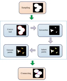
6. Particle counting

For pseudo agglomerates, the corresponding particles can be easily counted by using the

one-to-many relationship of label processing. However, for true agglomerates, it remains difficult to count the

number of primary particles involved in these agglomerates. By virtue of the analysis on IDC as shown

in Figure 4, it is proposed to use the concave points of the agglomerate contours to count the primary

round-like particles in these agglomerates. A fast algorithm is therefore given as illustrated in Figure

7, based on the morphology mask as follows.

Step 1. A toolbox algorithm 33 is used to figure out the convex hull (S ) for a true agglomerate, _ch

while the contour of S is entirely stuffed. _ch

Step 2. The concavities (S ) are computed as the difference between the convex hull (co S ) and ch

the agglomerate (S_ag), i.e., S_co S_chS_ag.

Step 3. The value of saliency Sal b is calculated for the boundary point ( ) b in the contour

image by

ci

( ) Mb

Sal b M

 ₍₃₇₎

where M is the pixel number of the circle mask centered on the boundary _ci b, and M is the _b

number of pixels in the maximum background block in the circle mask M . The mask center b scans

over the boundary of the contour by using a circle mask M with radius Rp. Salience points are

located in terms of Sal b( )0.7. If several continuous points comply with the condition, the point

Step 4. A concave point on the agglomerate boundary is determined if all the connecting lines

between the concave point and its adjacent salience points are inside the agglomerate.

Step 5. By drawing the nearest connecting lines between the determined concave points in

different concavities while avoiding any closed loop possibly constructed by the connecting lines, the

number of primary particles involved in these agglomerates is counted as the number of these

connecting lines plus one.

7. Experimental results

A seeded KDP cooling crystallization experiment was performed to verify the effectiveness of the

proposed image analysis method for recognizing pseudo agglomerates. The KDP solution was firstly

heated up to 40 °C and maintained at the temperature for an hour to ensure complete dissolution of the

solute. Then the solution was cooled down with a cooling rate of 0.3°C/min. The crystal seeds were

added shortly after the solution went into the supersaturated zone. The agitator was operated at a speed

of 150 rpm to keep all particles in suspension during the cooling crystallization process for image

monitoring. The aforementioned non-invasive microscopic imaging system was applied for in-situ

imaging, by using two LED lights with an illumination level of 400lux. In the double-view imaging

system, each image was taken at the pixel resolution of 2448×2048 per second. Note that 30 particles

were chosen from the previously captured images as the IDC training set to establish the classification

rule of preliminary sieving in advance.

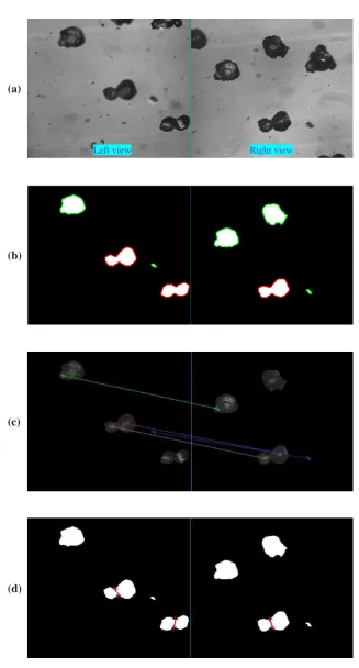
Considering the in-situ captured double-view images shown in Figure 2, the image analysis

method is illustrated in Figure 8. Firstly, the preprocessed images are shown in Figure 8 (a) by using

the reduction approach presented in Section 3. Then Figure 8 (b) shows the result by removing the

image background. Figure 8 (c) shows the segmented double-view image where the particle intensity

and the background are denoted by 1 and 0, respectively. Note that each pairs of double-view images

were simultaneously processed throughout the proposed analysis procedure. Figure 8 (d) shows the

candidate agglomerate recognized by the preliminary sieving using the IDC indices as listed in the

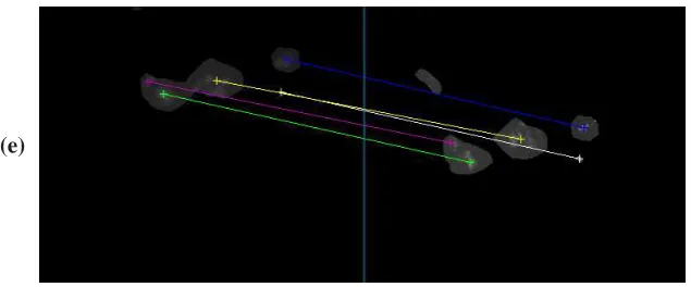
figure. Subsequently, Figure 8 (e) shows the pseudo agglomerate recognized by using the proposed

2

R . Note that all the valid particles and interest points were rightly matched between the

double-view images.

To compare the matching performance for the in-situ double-view images captured during the

crystallization process, the developed algorithms, SIFT 22, ASIFT 23, SURF 24 and ORB 25, were also

performed for Figure 2 based on the above image preprocessing and preliminary sieving. The

parameter of Gaussian function in SIFT and ASIFT was taken as 1.6, the parameters of SURF were

computed in terms of (16) in Section 5, and the parameters of ORB were chosen with the radius of

neighborhood being 3 and the edge threshold being 31, according to the guidelines given therein. Note

that the proposed outlier detection algorithm was performed beforehand to perform these algorithms

for fair comparison. The matching results are shown in Figure 9. It is seen that none of these algorithms

could give perfect matching for all the particles including the agglomerate. Figure 9 (a) shows that

SIFT gives correct matching for most of the interest points as shown in Figure 8 (e), but a prominent

interest point was overlooked as indicated by the yellow circle. In Figure 9 (b), it is obvious that a valid

particle was not matched in the double-view images by using ASIFT. Figure 9 (c) shows that there is

a mismatch of an interest point by using SURF, as indicated by the red line. Figure 9 (d) shows that a

valid particle is not matched while there exists a mismatch of an interest point (indicated by the purple

line) by using ORB.

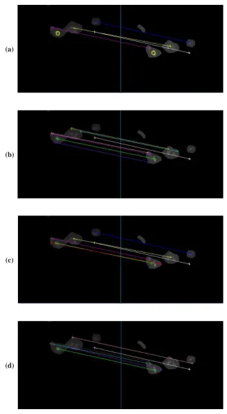
To further demonstrate the effectiveness of the proposed algorithm for recognizing particle

agglomeration and counting the number of primary particles, Figure 10 shows the imaging analysis

results for another pair of double-view images captured from the crystallization process, which

includes true agglomeration. It is seen from Figure 10 (b) that the candidate agglomerates were

recognized by using the preliminary sieving step, as indicated by the red contours. Then it is verified

in Figure 10 (c) by using the proposed feature matching algorithm that there are two agglomerates in

the left view. From Figure 10 (d) it is seen that the number of the primary particles involved in the

agglomerates is properly counted by the proposed algorithm.

Table 1 lists the recognition results for two different cases shown in Figure 8 and Figure 10,

respectively, for pseudo and true agglomerates. It can be seen that the proposed image analysis method

number of unagglomerated particles and the number of primary particles involved in the agglomerates

are rightly counted, respectively.

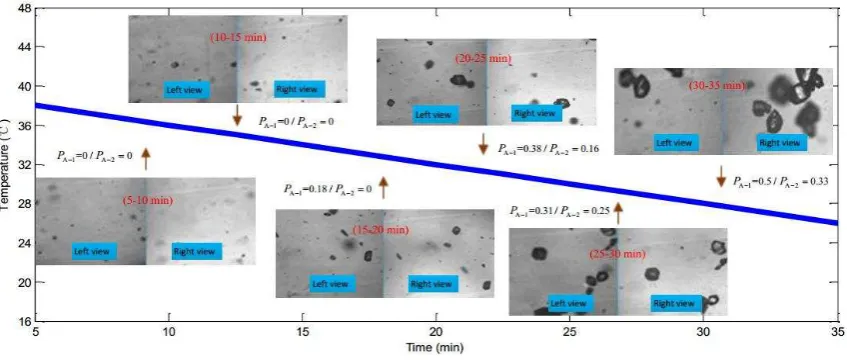
In addition, to demonstrate the effectiveness of the proposed method for on-line monitoring the

crystallization process, thirty pairs of double-view images including more than 200 particles captured

from the crystallization experiment, as illustrated in Figure 11 (including 6 representative pairs of

double-view images taken at different time instants), were taken to verify the proposed feature

matching algorithm in comparison with the above algorithms. For 6 representative pairs of these

images, the agglomeration degree defined in (1) is evaluated by using the proposed double-view

analysis, which is denoted by P_{A 2} in Figure 11. For comparison, the corresponding result given by

using the single-view analysis method 18, 20 _{is denoted by}

A 1

P _ in Figure 11. It is seen that the proposed

double-view analysis gives proper assessment of the agglomeration degree in real time (made per 5

minutes during the crystallization process), compared to the single-view analysis that gives obvious

misestimate such as the result for the image taken at the moment denoted by (15-20min). In other

words, the real-time estimation error arising from particle overlapping is significantly reduced by using

the proposed double-view analysis.

To evaluate the matching effect, the particle recall ratio P_pr is defined by

pa pr

pa pm

N P

N N



 (38)

where N_pa is the number of matched particles and N_pm is the number of unmatched particles.

The matching accuracy of interest points is defined by

a pm

t N P

N

 ₍₃₉₎

where N is the number of correct point matches and _a N is the total number of point matches. Note _t

that a valid particle is recognized if the point matching for two double-view images of the particle is

over 80%.

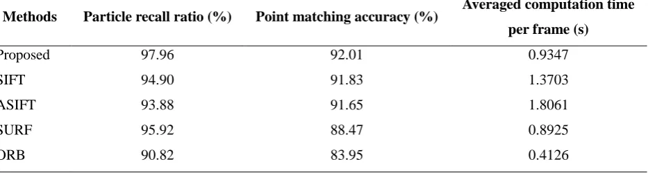
Three indices including point matching accuracy, particle recall ratio and averaged computation

time per frame were computed for comparison as listed in Table 2. Note that all of the above algorithms

used the same global nearest neighbor searching method 24 for computation. It is seen in Table 2 that

using a moderate computation time for each frame of double-view images. In contrast, SIFT and

ASIFT gave similar point matching accuracy close to that of the proposed algorithm. However, they

required an evidently longer computation time compared to the proposed algorithm, due to the use of

high-dimensional feature descriptors. Although ORB spent the shortest computation time in these

algorithms, the resulting point matching accuracy and particle recall ratio were the lowest compared

to the other algorithms, due to insufficient description of local features. By using a computation time

similar to the proposed algorithm, SURF gave inferior point matching accuracy, by using less local

texture features compared to the proposed algorithm. Note that for monitoring the crystallization

process, the particle recall ratio reflecting particle matching is more important than the other two

indices for agglomerate recognition. The result in Table 2 well demonstrates that the proposed

algorithm can give good matching and recognition for on-line monitoring particle agglomeration.

8. Conclusions

Based on an in-situ installed double-view imaging system, a synthetic image analysis method has

been proposed in this paper for monitoring particle agglomeration during a crystallization process. A

fast image segmentation approach based on image reduction is firstly adopted to perform image

preprocessing so as to reduce the influence from uneven illumination background and solution

turbulence. By defining an IDC index to detect possible agglomeration, a preliminary sieving

algorithm is given to screen out candidate agglomerates from preprocessed images, effectively

mitigating the on-line computation load. Then by introducing two texture descriptors, DCLBP and

MDLBP, for pattern recognition, a fast feature matching algorithm is developed to recognize pseudo

agglomerates with good accuracy. Subsequently, an efficient particle counting algorithm is established

to assess the agglomeration degree, by which both the unagglomerated particles and the primary

particles involved in agglomerates can be precisely counted, respectively. Experimental tests on

monitoring the KDP crystallization process well demonstrate that the proposed strategy can be more

effectively used for monitoring the crystal agglomeration degree in comparison with the existing

single-view analysis, along with obvious superiority for particle matching between double-view

Acknowledgment

This work was supported in part by the NSF China Grant 61633006 and the National Thousand

References

(1) Li, M.; Wilkinson, D.; Patchigolla, K., Determination of non-spherical particle size distribution from chord length measurements. Part 2: Experimental validation. Chemical Engineering Science 2005, 60, (18), 4992-5003.

(2) Yu, Z.; Chew, J.; Chow, P.; Tan, R., Recent advances in crystallization control: an industrial perspective. Chemical Engineering Research and Design 2007, 85, (7), 893-905.

(3) Nagy, Z. K.; Fevotte, G.; Kramer, H.; Simon, L. L., Recent advances in the monitoring, modelling and control of crystallization systems. Chemical Engineering Research and Design 2013, 91, (10), 1903-1922. (4) Zhang, B.; Willis, R.; Romagnoli, J. A.; Fois, C.; Tronci, S.; Baratti, R., Image-based multiresolution-ANN approach for online particle size characterization. Industrial & Engineering Chemistry Research 2014, 53, (17), 7008-7018.

(5) Schorsch, S.; Ochsenbein, D. R.; Vetter, T.; Morari, M.; Mazzotti, M., High accuracy online measurement of multidimensional particle size distributions during crystallization. Chemical Engineering Science 2014, 105, (2), 155-168.

(6) Zhou, Y.; Srinivasan, R.; Lakshminarayanan, S., Critical evaluation of image processing approaches for real-time crystal size measurements. Computers & Chemical Engineering 2009, 33, (5), 1022-1035.

(7) Li, P.; He, G.; Lu, D.; Xu, X.; Chen, S.; Jiang, X., Crystal size distribution and aspect ratio control for rodlike urea crystal via two-dimensional growth evaluation. Industrial & Engineering Chemistry Research 2017, 56, (9), 2573-2581.

(8) Wang, X. Z.; Roberts, K. J.; Ma, C., Crystal growth measurement using 2D and 3D imaging and the perspectives for shape control. Chemical Engineering Science 2008, 63, (5), 1173-1184.

(9) Zhou, Y.; Lakshminarayanan, S.; Srinivasan, R., Optimization of image processing parameters for large sets of in-process video microscopy images acquired from batch crystallization processes: Integration of uniform design and simplex search. Chemometrics & Intelligent Laboratory Systems 2011, 107, (2), 290-302.

(10) Schorsch, S.; Vetter, T.; Mazzotti, M., Measuring multidimensional particle size distributions during crystallization. Chemical Engineering Science 2012, 77, (1), 130-142.

(11) Chen, X.; Zhou, W.; Cai, X.; Su, M.; Liu, H., In-line imaging measurements of particle size, velocity and concentration in a particulate two-phase flow. Particuology 2014, 13, (2), 106-113.

(12) Zhang, R.; Ma, C. Y.; Liu, J. J.; Wang, X. Z., On-line measurement of the real size and shape of crystals in stirred tank crystalliser using non-invasive stereo vision imaging. Chemical Engineering Science 2015, 137, (10), 9-21.

(13) Larsen, P. A.; Rawlings, J. B., The potential of current high-resolution imaging-based particle size distribution measurements for crystallization monitoring. AIche Journal 2009, 55, (4), 896-905.

(14) Huo, Y.; Liu, T.; Liu, H.; Ma, C. Y.; Wang, X. Z., In-situ crystal morphology identification using imaging analysis with application to the L-glutamic acid crystallization. Chemical Engineering Science 2016, 148, (12), 126-139.

(15) Zhang, R.; Ma, C. Y.; Liu, J. J.; Zhang, Y.; Liu, Y. J.; Wang, X. Z., Stereo imaging camera model for 3D shape reconstruction of complex crystals and estimation of facet growth kinetics. Chemical Engineering Science

2017, 160, 171-182.

(16) Ulrich, J.; Frohberg, P., Problems, potentials and future of industrial crystallization. Frontiers of Chemical Science and Engineering 2013, 7, (1), 1-8.

(17) Ålander, E. M.; Uusi-Penttilä, M. S.; Rasmuson, Å. C., Characterization of paracetamol agglomerates by image analysis and strength measurement. Powder Technology 2003, 130, (1), 298-306.

(19) Terdenge, L. M.; Heisel, S.; Schembecker, G.; Wohlgemuth, K., Agglomeration degree distribution as quality criterion to evaluate crystalline products. Chemical Engineering Science 2015, 133, (8), 157-169. (20) Ochsenbein, D. R.; Vetter, T.; Schorsch, S.; Morari, M.; Mazzotti, M., Agglomeration of needle-like crystals in suspension: I. Measurements. Crystal Growth & Design 2015, 15, (4), 1923-1933.

(21) Borchert, C.; Temmel, E.; Eisenschmidt, H.; Lorenz, H.; Seidelmorgenstern, A.; Kai, S., Image-based in situ identification of face specific crystal growth rates from crystal populations. Crystal Growth & Design 2014, 14, (3), 952–971.

(22) Lowe, D. G., Distinctive image features from scale-invariant keypoints. International Journal of Computer Vision 2004, 60, (2), 91-110.

(23) Morel, J. M.; Yu, G., ASIFT: A new framework for fully affine invariant image comparison. Siam Journal on Imaging Sciences 2009, 2, (2), 438-469.

(24) Bay, H.; Ess, A.; Tuytelaars, T.; Gool, L. V., Speeded-up robust features (SURF). Computer Vision & Image Understanding 2008, 110, (3), 346-359.

(25) Rublee, E.; Rabaud, V.; Konolige, K.; Bradski, G. In ORB: An efficient alternative to SIFT or SURF, International Conference on Computer Vision, 2011; 2011; pp 2564-2571.

(26) Ojala, T.; Pietikäinen, M.; Mäenpää, T., Multiresolution gray-scale and rotation invariant texture classification with local binary patterns. IEEE Transactions on Pattern Analysis & Machine Intelligence 2002, 24, (7), 971-987.

(27) Liu, L.; Fieguth, P.; Guo, Y.; Wang, X.; Pietikäinen, M., Local binary features for texture classification: Taxonomy and experimental study. Pattern Recognition 2017, 62, 135-160.

(28) Guo, Z.; Zhang, L.; Zhang, D., A completed modeling of local binary pattern operator for texture classification. IEEE Transactions on Image Processing 2010, 19, (6), 1657-63.

(29) Guo, Z.; Zhang, L.; Zhang, D., Rotation invariant texture classification using LBP variance (LBPV) with global matching. Pattern Recognition 2010, 43, (3), 706-719.

(30) Liu, L.; Zhao, L.; Long, Y.; Kuang, G.; Fieguth, P., Extended local binary patterns for texture classification. Image & Vision Computing 2012, 30, (2), 86-99.

(31) Yang, G.; Kubota, N.; Sha, Z.; Louhi-kultanen, M.; Wang, J., Crystal shape control by manipulating supersaturation in batch cooling crystallization. Crystal Growth & Design 2006, 6, (12), 2799-2803.

(32) Nývlt, J.; Karel, M., Crystal agglomeration. Crystal Research and Technology 1985, 20, (2), 173-178. (33) Gonzales, R. C.; Woods, R. E.; Eddins, S. L., Digital image processing using MATLAB. Pearson Prentice Hall: Upper Saddle River, NJ, 2004.

(34) Chen, J.; Wang, X. Z., A wavelet method for analysis of droplet and particle images for monitoring heterogeneous processes. Chemical Engineering Communications 2005, 192, (4), 499-515.

(35) Oyallon, E.; Rabin, J., An analysis of the SURF method. Image Processing On Line 2015, 5, (337), 176-218.

(36) Cai, D.; He, X.; Han, J. In Spectral regression for efficient regularized subspace learning, International Conference on Computer Vision, 2007; 2007; pp 1-8.

(37) Arya, S.; Mount, D. M.; Netanyahu, N. S.; Silverman, R.; Wu, A. In An optimal algorithm for approximate nearest neighbor searching, Acm-Siam Symposium on Discrete Algorithms. 23-25 January 1994, Arlington, Virginia, 1994; 1994; pp 573-582.

List of Table and Figure Captions

Table 1. Recognition results for two different cases

Table 2. Comparison of matching results by using different algorithms

Figure 1. (a) Schematic of a microscopic image monitoring system for crystallization monitoring;

(b) Experimental set-up of a non-invasive microscopic double-view imaging system

Figure 2. In-situ double-view images captured by a microscopic imaging system

Figure 3. Flowchart of the proposed method for agglomeration detection

Figure 4. Illustration of IDC: (a) an unagglomerated particle; (b) agglomerate of two particles;

(c) agglomerate of three particles; (d) agglomerate of four particles

Figure 5. Flowchart of the proposed feature matching algorithm

Figure 6. Comparison of texture recognition: (i) three different texture patterns (a, b, c); (ii) LBP

(a1, b1, c1); (iii) VAR values (a2, b2, c2); (iv) DCLBP (a3, b3, c3); (v) MDLBP (a4, b4,

c4)

Figure 7. Schematic of the proposed counting algorithm for particle agglomeration

Figure 8. Double-view image processing for in-situ captured images: (a) preprocessed images; (b)

result after removing the background; (c) segmented result; (d) preliminary sieving with

IDC (a candidate agglomerate is labeled in red contour); (e) feature matching (the

candidate agglomerate in the left view corresponds to two particles in the right view)

Figure 9. Comparison of matching results: (a) SIFT; (b) ASIFT; (c) SURF; (d) ORB

Figure 10. Agglomerate recognition and particle counting results: (a) in-situ captured double-view

images; (b) preliminary sieving (candidate agglomerates are labeled with red contour);

(c) feature matching; (d) counting primary particles in the agglomerates (the connecting

lines indicating four primary particles in the two agglomerates in the left view)

Table 1. Recognition results for two different cases

Target parameters in the double-view images Case 1 Case 2

The number of pseudo agglomerates 1 0

The number of true agglomerates 0 2

The number of unagglomerated particles 5 3

The number of primary particles involved in the agglomerates 0 4

The total number of all the primary particles 5 7

The agglomeration degree 0% 57.14%

Table 2. Comparison of matching results by using different algorithms

Methods Particle recall ratio (%) Point matching accuracy (%) Averaged computation time per frame (s)

Proposed 97.96 92.01 0.9347

SIFT 94.90 91.83 1.3703

ASIFT 93.88 91.65 1.8061

SURF 95.92 88.47 0.8925

(a) (b)

Figure 1. (a) Schematic of a microscopic image monitoring system for crystallization monitoring; (b)

Experimental set-up of a non-invasive microscopic double-view imaging system

(a) Left view (b) Right view

Figure 2. In-situ double-view images captured by a microscopic imaging system

In-situ double-view imaging

Real-time assessment of agglomeration degree

Image preprocessing

Preliminary sieving

Feature matching

Particle counting Step 1

Step 2

Step 3

Step 4

Figure 3. Flowchart of the proposed method for agglomeration detection

IDC=0.3522 IDC=0.3061 IDC=0.3028 IDC=0.2901

(a) (b) (c) (d)

Figure 4. Illustration of IDC: (a) an unagglomerated particle; (b) agglomerate of two particles; (c) agglomerate of

Interest point

Haar MDLBP DCLBP

Location

Histogram Orientation Description

Matching

×

Dimension reduction KD tree

searching Outlier detection

Result _{× ×}

×

H

v v_M vD vO

(i) 66 58 56 64 62 68 66 63 60 182 5 12 250 193 80 248 126 60 248 12 5 250 126 80 182 193 60 Original Texture Pattern

(a) (b) (c)

(ii) 1 0 0 1 1 1 1 1 1 0 0 1 1 1 1 1 1 0 0 1 1 1 1 1 LBP

(a1) (b1) (c1)

(iii) VAR _{15.8 8333.8} 8333.8

(a2) (b2) (c2)

(iv) 1 0 0 1 0 1 1 1 1 0 0 1 1 0 1 0 1 0 0 1 0 0 1 1 DCLBP

(a3) (b3) (c3)

(v) 1

1 0 0 0 0 1 1 0 1 0 0 1 0 0 1 0 1 0 0 1 0 0 1 1 MDLBP

(a4) (b4) (c4)

Sampling

Convex

hull Concavities

Concavities

Salient points

Salient points

Concave points

Concave points

Connecting

(a)

(b)

(c)

(e)

Figure 8. Double-view image processing for in-situ captured images: (a) preprocessed images; (b) result after

removing the background; (c) segmented result; (d) preliminary sieving with IDC (a candidate agglomerate is labeled in red contour); (e) feature matching (the candidate agglomerate in the left view corresponds to two

(a)

(b)

(c)

(d)

(a)

(b)

(c)

(d)

Figure 10. Agglomerate recognition and particle counting results: (a) in-situ captured double-view images;

(b) preliminary sieving (candidate agglomerates are labeled with red contour); (c) feature matching; (d) counting primary particles in the agglomerates (the connecting lines indicating four primary particles in the two

agglomerates in the left view)