Numerical modelling of hydro-morphological processes dominated by fine suspended sediment in a stormwater pond

Research papers

Numerical modelling of hydro-morphological processes dominated by

fine suspended sediment in a stormwater pond

Mingfu Guan

a,⇑

, Sangaralingam Ahilan

b,e

, Dapeng Yu

a

, Yong Peng

c,1

, Nigel Wright

d a_{Department of Geography, Loughborough University, Loughborough, UK}

b

Centre for Water Systems, University of Exeter, Exeter, UK c

State Key Laboratory for Hydraulics and Mountain River Engineering, Sichuan University, China d

Faculty of Technology, De Montfort University, Leicester, UK e

Water@Leeds and School of Civil Engineering, University of Leeds, Leeds, UK

a r t i c l e i n f o

Article history: Received 23 May 2017

Received in revised form 7 September 2017 Accepted 3 November 2017

Available online 7 November 2017 This manuscript was handled by Dr Marco Borga, Editor-in-Chief, with the assistance of Jennifer Guohong Duan, Associate Editor

Keywords:

Shallow water equations Suspended load Morphological changes Stormwater pond

a b s t r a c t

Fine sediment plays crucial and multiple roles in the hydrological, ecological and geomorphological func-tioning of river systems. This study employs a two-dimensional (2D) numerical model to track the hydro-morphological processes dominated by fine suspended sediment, including the prediction of sediment concentration in flow bodies, and erosion and deposition caused by sediment transport. The model is gov-erned by 2D full shallow water equations with which an advection–diffusion equation for fine sediment is coupled. Bed erosion and sedimentation are updated by a bed deformation model based on local sed-iment entrainment and settling flux in flow bodies. The model is initially validated with the three laboratory-scale experimental events where suspended load plays a dominant role. Satisfactory simula-tion results confirm the model’s capability in capturing hydro-morphodynamic processes dominated by fine suspended sediment at laboratory-scale. Applications to sedimentation in a stormwater pond are conducted to develop the process-based understanding of fine sediment dynamics over a variety of flow conditions. Urban flows with 5-year, 30-year and 100-year return period and the extreme flood event in 2012 are simulated. The modelled results deliver a step change in understanding fine sediment dynamics in stormwater ponds. The model is capable of quantitatively simulating and qualitatively assessing the performance of a stormwater pond in managing urban water quantity and quality.

Ó2017 The Author(s). Published by Elsevier B.V. This is an open access article under the CC BY license (http://creativecommons.org/licenses/by/4.0/).

1. Introduction

In river systems, fine-grained sediment is a natural and essen-tial component and plays a crucial role in the hydrological, ecolog-ical and geomorphologecolog-ical functioning of the system. It has been recognised that fine-grained sediment management in urban rivers is environmentally significant (Birch et al., 2006). Sustainable sed-iment management requires a structure of supporting research on fine sediment dynamics and its interactions within hydrological catchments such as rivers, floodplains, reservoirs and Sustainable Urban Drainage Systems (SuDS) (Owens et al., 2005).

In general, fine-grained sediment has a controlling influence on the quality and quantity of receiving water. In an urban catchment, contaminants and pollutants including heavy metals and nutrients are generally absorbed by fine sediment which is then conveyed to

the receiving waters (Saeedi et al., 2004; Jartun et al., 2008; Jones et al., 2008). These urban pollutants attached to sediments have implications on both habitats of downstream receiving waters and human health (Wood and Armitage, 1997; Owens et al., 2005; Crosa et al., 2010). To mitigate these risks, more sustainable features, such as stormwater ponds, are increasingly used in urban catchments as an option to manage fine suspended sediments (Ahilan et al., 2016; Allen et al., 2017) by storing stormwater run-off, trapping fine sediments and improving urban runoff quality. The movement of sediment will be minimised by the interrupted flows in a storm water pond. The low energy environment in the pond enables the considerable proportion of fine suspended load is trapped which provides water quality benefits to receiving water bodies. However, from a longer-term viewpoint, this will diminish the storage capacity of stormwater ponds, thereby influencing their hydraulic performance and maintenance. Similarly, fine-grained sedimentation occurs in dam reservoirs where the release of deposited sediments often leads to cascading effects in down-stream reaches through sediment transport and re-deposition

https://doi.org/10.1016/j.jhydrol.2017.11.006

0022-1694/Ó2017 The Author(s). Published by Elsevier B.V.

This is an open access article under the CC BY license (http://creativecommons.org/licenses/by/4.0/).

⇑ Corresponding author.

E-mail addresses: [email protected](M. Guan),[email protected] (Y. Peng).

1 _{College of Water Resources and Hydropower, Sichuan University, China.}

Contents lists available atScienceDirect

Journal of Hydrology

(Liu et al., 2004). This has been considered to be a worldwide prob-lem (Vörömarty et al. (2003)). Additionally, excessive suspended sediment inputs to rivers due to catchment erosion and in-channel bank erosion can cause sedimentation in in-channels which may affect channel morphology, stream habitats and navigation (Eekhout et al., 2015). In view of the sediment effects, natural pro-cesses have been widely used for river and flood management in recent years (Dadson et al., 2017). In the aforementioned cases, fine suspended sediment has a controlling influence on the quality and quantity of receiving waters in hydro-systems through playing a variety of roles. Therefore, there is a need to develop an improved understanding of how fine-grained sediment is eroded, trans-ported and deposited by a variety of flow environments.

In recent years, numerical models have been increasingly used to understand complex flows, sediment transport and the corre-sponding morphological changes in rivers, floodplains and SuDS. In view of the multiple roles of fine-grained sediment in receiving waters, a robust fine sediment model is crucial to develop coupled models enabling the simulations and understanding of hydrologi-cal, ecological and geomorphological conditions of catchments. Recently numerical models have been used to simulate dam-break induced in-channel evolution (Cao et al., 2004; Simpson and Castelltort, 2006; Bohorquez and Fernandez-Feria, 2008, Zech et al., 2008; Guan et al., 2015a; Benkhaldoun et al., 2012; Li and Duffy, 2012; Guan et al., 2014), sediment routing in dam reservoirs (Liu et al., 2004; Guertault et al., 2016), turbidity currents over erodible bed (Hu and Cao, 2009; Hu et al., 2012; Janocko et al., 2013). This provides feasible mathematical modelling approaches to quantify the evolution of sediment-laden flows and correspond-ing geomorphological changes dominated by fine-grained sediment.

This research presents a 2D numerical tool to track the erosion, transport and deposition of fine-grained sediment and particularly investigate fine sediment dynamics in stormwater ponds. The model is a depth-averaged 2D numerical model that includes a robust shallow water based hydrodynamic model, a suspended load transport model and a bed evolution model. It provides more reliable information than a 1D model whilst being more cost-effective than a 3D model. The model is capable of simulating full sediment transport process where non-cohesive fine suspended load plays a dominant role, including both sediment concentration in flow bodies and bed changes. This is not only limited to a case with full suspended load transport, but also to a case which may have a small portion of bedload. Whatever, this should have a small rouse number lower than 2.5 during the main transport stage. The model is firstly validated against three laboratory-scale experiments prior to a real-world application in a stormwater pond located in Newcastle Great Park, UK. Based on the simulation results, this study aims to determine the erosion, transport and deposition characteristics of fine sediment in a stormwater pond with various flow conditions and to develop a greater understand-ing of fine-grained sediment dynamics in stormwater ponds.

2. Numerical model

2.1. Hydrodynamic model

Shallow water based numerical models have been widely used for hydraulic modelling due to their robustness in capturing flow hydraulics (Guan et al., 2013; Vacondio et al., 2014; Costabile and Macchione, 2015; Hou et al.,2015; Guan et al., 2015b). The 2D shallow water equations can be expressed by:

@

g

@tþ

@hu @x þ

@h

v

@y ¼0 ð1aÞ

@hu @t þ

@ @x hu

2_þ1 2gh

2

þ@hu

v

@y

¼@hTxx

@x þ @hTyx

@y gh @zb

@x ghSfxþ

D

qu

q

@zb

@t

D

qgh

2 2q

@C

@x ð1bÞ

@hu @t þ

@hu

v

@x þ

@ @y h

v

2_þ1 2gh

2

¼@hTxy

@x þ @hTyy

@y gh @zb

@yghSfyþ

D

q

v

q

@zb

@t

D

qgh

2 2q

@C

@y ð1cÞ

where h= flow depth, zb= bed elevation,

g

=h+zb denotes the water surface elevation which includes both changes of the water depth and bed elevation varying with the time t, u and v= the depth-averaged flow velocity components in the two Cartesian directions, g= acceleration due to gravity, p= sediment porosity, C= total volumetric sediment concentration,

q

sand

q

wdenote the densities of sediment and water respectively,D

q

=

q

s

q

w,

q

= den-sity of flow-sediment mixture,Sfx,Sfy= frictional slope inxandy components which are calculated based on Manning’s roughness

coefficient n bySfx¼n 2_upffiffiffiffiffiffiffiffiffiffi_u2_þv2

h4=3 ;Sfy¼n

2vpffiffiffiffiffiffiffiffiffiffi_u2_þv2

h4=3 , Txx, Txy, Tyx and Tyy

are the depth-averaged turbulent stresses which are determined by the Boussinesq approxi

v

mation which has been widely used in the literature (e.g. Wu, 2004; Abad et al., 2008; Begnudelli et al., 2010). This gives the Reynolds stresses as:

Txx¼ 2ðmtþ

mÞ

@

u

@x ð2aÞ

Txy¼Tyx¼ ðmtþ

mÞ

@

u @xþ

@

v

@x

ð2bÞ

Tyy¼ 2ðmtþ

mÞ

@

v

@x ð2cÞ

where

v

tis the turbulence eddy viscosity and is the molecular vis-cosity which can be ignored in environmental applications. Various approaches have been adopted to estimate the turbulence viscosity, e.g. assuming a constant eddy viscosity, an algebraic turbulence model (

m

thu

), as well as thek–

e

turbulence model. In this study, the eddy viscosity is estimated by

m

t¼bhuwithb= 0.5.

2.2. Fine suspended load model

The suspended load transport is governed by the advection–dif-fusion equation. For non-uniform graded sediment mixtures, it is necessary to divide the graded sediments into fractions due to the difference of grain-size related parameters (Guan et al., 2015b). For the suspended transport of each fraction, the governing equation is described by

@hCi

@t þ @huCi

@x þ @h

v

Ci

@y ¼ @ @x

e

sh

@Ci

@x

þ @ @y

e

sh

@Ci

@y

þ ðSE;i

SD;iÞ ð3Þ

where

es

is the diffusion coefficient of sediment particles;SE,iis the entrainment flux of sediment for the ith fraction;SD,iis the deposi-tion flux of sediment of the ith fracdeposi-tion. The diffusion coefficient of sediment particles is related to the diffusion of fluid momentum, and it is determined by using the below formula presented invan Rijn (1984).

e

s¼b/mt ð4Þ

of the fluid turbulence by the sediment particles and it is assumed to be dependent on the local sediment concentration. Both factors are calculated by using the formula derived by van Rijn (1984), which are widely used (e.g.Duan and Nanda, 2006).

b¼1þ2

x

f u

2

for 0:1<

x

f

u <1

/¼1þ Ca

Cae

0:8 2 Ca

Cae

0:4

where Ca is the near-bed concentration at the reference level a (average for non-uniform sediments);Caeis the near bed equilib-rium concentration (average for non-uniform sediments). Both are defined below. As there is no universal theoretical expression for the entrainment flux and deposition flux of sediments, both vari-ables are calculated by the following widely-used function.

SE;i¼Fi

x

f;iCae;i; SD;i¼Fi

x

f;iCa;i ð5Þ

where Fi, percentage of the ith grain fraction;

x

f,i,is the effective settling velocity for the ith grain fraction which is calculated by the function derived bySoulsby (1997)as below;

x

f;i¼

m

di

½ ffiffiffiffiffiffiffiffiffiffiffiffiffiffiffiffiffiffiffiffiffiffiffiffiffiffiffiffiffiffiffiffiffiffiffiffiffiffiffiffiffiffiffiffiffiffiffiffiffiffiffiffiffiffiffiffiffiffiffi10:362_{þ ð1C}

iÞ

4:7 1:049d3 q

10:36 ð6Þ

Ca,i=dCiis the near-bed concentration for the ith grain frac-tion at the reference level a; the definifrac-tion of the coefficient d byCao et al., (2004) is:d¼minf2:0;ð1pÞ=Cg; Cae,iis the near bed equilibrium concentration for the ith_{grain fraction at the} ref-erence level that is calculated by using the van Rijn formula (van Rijin, 1984). For each grain fraction, the function can be expressed as:

Cae;i¼0:015

d50 a

T1:5 d0:3

ð7Þ

T¼ðu; 2

u2;crÞ

u2

;cr

a¼min½maxðks;2d50;0:01hÞ;0:2h

whereksis the equivalent roughness height;d⁄=di[(

q

s/

q

w1)g/

m

2_]1/3_{is the dimensionless particle diameter;}

_m

_{is the viscosity of} water;u;

¼uð ffiffiffig p

=C0Þ is bed-shear velocity related to grain; C’is the Chézy-coefficient related to grain; u;cr¼

ffiffiffiffiffiffiffiffiffiffiffiffiffiffiffiffiffiffiffiffiffiffiffiffi

ðs1Þgdhc p

is the critical bed-shear velocity, wherehcis the Shields shear stress.

2.3. Morphological change model

Morphological evolution is determined by the difference of sed-iment entrainment and deposition that is calculated per grid cell at each time step. The equation used to calculate morphological change is written by

@zb

@t ¼ XN

i¼1 @zb

@t

i

¼ 1

1p XN

i¼1ðSD;iSE;iÞ ð8Þ

whereNis the number of grain size fractions.

2.4. Numerical method

Eqs.(1)and(3) and (8)constitute the model system which is a shallow water non-linear system. In compact form, the governing equations can be expressed by

@U @t þ

@E @xþ

@F @y¼

@E~ @xþ

@~F

@yþS ð9Þ

where U¼

g

hu h

v

hCi 2 66 66 66 4 3 77 77 77 5

; E¼ hu hu2þ1

2gh 2 hu

v

hCi 2 66 66 66 4 3 77 77 77 5

; F¼ hu hu

v

h

v

2þ1

2gh 2 hCi 2 66 66 66 4 3 77 77 77 5 ; ~ E¼ 0 hTxx hTxy

e

xh@_@C_xi

2 66 66 66 4 3 77 77 77 5

; ~F¼ 0 hTyx

hTyy

e

yh@_@C_yi

2 66 66 66 4 3 77 77 77 5 S¼ 0 gh@zb

@xghSfxþDq u

q @

zb

@tD

qgh2 2q @@Cx

gh@zb

@yghSfyþD

qv q @

zb

@t

Dqgh2 2q @

C

@y

ðSE;iSD;iÞ

0 B B B B B B B B @ 1 C C C C C C C C A

whereUis the vector of conserved variables;EandFare the flux vectors of the flow in the xandydirections respectively,E~and~F contain the turbulent terms in thexandydirections,Sis the source term vector.

The model is solved numerically by a well-balanced Godunov-type finite volume method (FVM) based on Cartesian coordinates. To update the variables in each cell, the following equation is used to update hydrodynamics:

Uni;þj1¼U n i;j

D

t

D

xðE

i;jE~i;jÞ

D

t

D

yðF

i;j~Fi;jÞ þ

D

tSi;j ð10Þ

where the vectorsEi;j¼E

iþ1=2;jE

i1=2;j,F

i;j¼F

i;jþ1=2F

i;j1=2are the difference of the fluxes at the left and right interfaces of the cell (i,j) in thexandydirection;~E_i;jand~F_i;jrepresents the flux difference of turbulent and dispersion stresses at the left and right interfaces of the cell (i,j) in thexandydirection;Dt,Dx,Dyare the time step, cell size in thexandydirection, respectively. To calculate the first three flux terms (e.g. E_lr1;2;3), the Harten, Lax and van Leer (HLL) scheme has been used in this study. More details are described in

Guan et al., (2014). Similar to updating the hydrodynamic variables, the sediment concentration is updated at the same cell and time step based on the sediment inter-cell fluxC⁄as follows,

ctþDt i;j ¼c

t i;j

a

D

t

D

x c

iþ1 2;jc

i1 2;j

þ

D

t

D

y c

i;jþ1 2c

i;j1 2

þ

D

tScði;jÞ ð11Þ

wheretrepresents the time;Scis the source term shown in the right hand side of Eq.(3). The sediment fluxC⁄is calculated using the fol-lowing equation,

C¼cð iþjÞ ¼

ðElrj1iþF

lrj1jÞclSP0 ðElrj1iþF

lrj1jÞcrS<0 8

> < >

: ð12Þ

3. Results and discussion

3.1. Model validation

Three laboratory cases were used to verify the model capability in simulating morphological changes dominant by fine suspended load, which includes (1) sediment transport in a trench, (2) partial dam-breach flow over a mobile channel, and (3) localised erosion and deposition in a pond with erodible bed. In all three experimen-tal cases, it has been observed that suspended load is the main transport mode, which ensures the applicability of the cases in the model verification. Here the model errors with the measured data were quantified using the Brier Skill Score (BSS) as:

BSS¼1 Xn

1 ðzo

izmiÞ

2

Xn

1 ðzo

i zoi;t¼0Þ 2

ð13Þ

where superscriptsmandorefer to modelled and observed point data, respectively, andnis the total number of point data.

3.1.1. Sediment transport in a trench

To verify the capability of the proposed model in predicting bed evolution under the conditions of unsteady flows a simulation was carried out to compare with experiments originally conducted at the Delft Hydraulics Laboratory to investigate the movable bed evolution caused by steady open channel flow (van Rijn, 1980). The trench is located in the middle of the 30 m long channel. Three tests with different side slopes of the trench (1:3, 1:7 and 1:10) were performed in the experiments. Following van Rijn (1980), the key information of the three tests is listed inTable 1. The mean inflow velocity was 0.51 m/s at the inlet and the water depth were kept constant as 0.39 m. The erodible bed consists of fine sand with d10= 0.115 mm,d50= 0.16 mm andd90= 0.2 mm. The sand density and porosity was 2650 kg/m3 _{and 0.4 respectively. According to} the experiment, the settling velocity of sediment particles was 0.013 m/s ± 25%. A hindering settling velocity

x

0= 0.015 m/s is used. Manning’s coefficient n is set to be 0.016. In addition, to maintain the sediment equilibrium conditions in the upstream, i.e. no scour or deposition occurring, sand with the same composi-tion was fed at a constant rate of 0.04 kg/s/m; thereby, the sus-pended load transport rate was estimated to be 0.03 ± 0.006 kg/s/ m and the bed load transport rate of about 0.01 kg/s/m. The contri-bution of the suspended load transport to the total load transport was in the range of 60% to 90%.

For simulation, the whole domain is discretised by 150 cells withDx= 0.2 m. To ensure steady flow, the model is run for 900 s. After 900 s, sand is fed and bed evolution occurs. Van Rijn (1984)suggested estimating the reference level by the following equation,a¼min½maxðks;2d50;0:01hÞ;0:2h. Based on this formu-lation,a= 0.01 m anda= 0.02 m was used in the model to

demon-strate the influence of the reference level.Fig. 1plots the simulated velocity and depth-averaged measurement at the five measured sections. It can be seen that the model produces the velocity rea-sonably well around the trench. Also, the water surface has been simulated to be close to the real constant value 0.39 m. Regarding the predictin of changes in bed profiles,Fig. 2indicates that the simulated bed profiles witha= 0.01 m anda= 0.02 m show similar shape with only a slight difference. With both reference levels, the simulated bed has a high Brier Skill Score which is over 0.9. When a= 0.01 m, the model gives a better results. Therefore, the model is also verified in Test 2 and Test 1 with the reference level a= 0.01 m. As shown in Fig. 3, the general bed profiles at both 7.5 h and 15 h are produced with a good BSS. This implies the capa-bility of the model in simulating bed changes due to sediment transport dominant by suspended load.

3.1.2. Partial dam-breach flow over a mobile channel

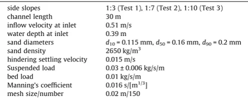
[image:4.595.327.527.69.186.2]

To verify and validate the performance of the suspended load model it was used to reproduce partial dam-breach flow experi-ments over a mobile bed, which were carried out at the Hydraulics Laboratory of Tsinghua University, China (Xia et al., 2010). A thin dam was located 2.0 m downstream of a 18.5 m1.6 m rectangu-lar flume, and a 0.2 m wide dam-breach centred at y = 0.8 m; the region of 4.5 m after dam site was covered by fine non-uniform coal ash with a median diameter of 0.135 mm, and its natural and dry density were measured approximately as 2248 kg/m3 and 720 kg/m3 _{respectively; the water depth was initially set to} be 0.4 m in the reservoir and 0.12 m downstream of the dam. In this experiment, the bed levels at two cross sections CS1 (x = 2.5 m) and CS2 (x = 3.5 m) after 20 s were measured. During the whole experiment, only suspended load transport occurs due to the particles being so fine.Table 2lists the key parameters used in the simulation. For the simulation, the domain is discretised by 37080 cells, and the time interval isDt= 0.005s. The Manning’s coefficient n= 0.02 s/[m1/3_{]; the sediment porosity is set as} 0.35. The suspended load model is run for 20 s.Fig. 4 shows a comparison between the observed and modelled cross-sectional profiles at 20 s. It is shown that the trend of the predicted bed pro-files is similar to that of the measured propro-files. Erosion occurs in the middle of the cross sections. The bed erosion quantity is less than the measurement at CS1 where the predicted bed is underes-timated, particularly in terms of the erosion width. However, a similar maximum scour depth and location are predicted here. At CS2, the simulated and measured bed profiles are in good agree-ment with each other. The simulated and measured scour depths are very close and the erosion areas agree very well with each other, but the measured range of bed profile is about 20 cm wider than the simulated range. For this reason, it can be seen that the BSS for CS2 is relatively smaller. The bed deposition is underesti-mated by the model here. This is possibly due to either the Table 1

Key parameters of the three tests.

side slopes 1:3 (Test 1), 1:7 (Test 2), 1:10 (Test 3)

channel length 30 m

inflow velocity at inlet 0.51 m/s water depth at inlet 0.39 m

sand diameters d10= 0.115 mm,d50= 0.16 mm,d90= 0.2 mm sand density 2650 kg/m3

hindering settling velocity 0.015 m/s Suspended load 0.03 ± 0.006 kg/s/m

bed load 0.01 kg/s/m

Manning’s coefficient 0.016 s/[m1/3 ] mesh size/number 0.02 m/150

-0,2 0 0,2 0,4 0,6

10 12,5 15 17,5 20

v

e

lo

cit

y

(m

/s

)

[image:4.595.34.282.650.751.2]

channel length (m) Initial bed measured simulated

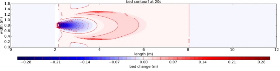
experimental errors or the neglected turbulence term, which means the model may not be able to generate the rapid formation of horizontal circulating flow at the downstream of the dam.Fig. 5

illustrates the contour plot of the simulated bed topography after 20 s. Severe erosion occurs at the outlet of the dam, and the eroded suspended load is flushed to deposit downstream due to the decrease of bed shear stress.

3.1.3. Erosion and deposition in a pond with erodible bed

The experiment was conducted to investigate the erosion pro-cess in a rectangular basin due to clear water inflow from a narrow channel byThuc (1991). In this test, the initial setup involves an inlet rectangular channel of 2.0 m long and 0.2 m wide, a rectangu-lar movable basin with 5.0 m long and 4.0 m wide, and a 1.0 m long and 1.2 m wide channel in the downstream. Therein, the movable basin consists of fine sand with median diameter of 0.6 mm, with a movable bed layer was 0.16 m thick. For the initial hydraulic con-ditions, initial water depth was specified as 0.15 m; the inflow velocity at the inflow boundary was kept constant at 0.6 m/s, and the water depth at the outlet was a constant value of 0.15 m. Only basin area is erodible during the experiment period.Table 3show the key parameters of the experimental case. This experiment is simulated in this study because the sediment particle diameter is small (0.6 mm), and the rouse number of the case is estimated to be in a range of 0–2.4 in the main movable area, which means sus-pended load is the dominant transport mode. This fits the capabil-ity of the present model.

The length of channel is discretised with a constant interval

Dx = 0.1 m, but in width direction, the grid spacing around the

-0,2 -0,1 0 0,1 0,2 0,3 0,4 0,5

11 14 17 20 23

elev

ation (m

)

channel length (m) Initial bed Water surface Measured at t=7.5h a=0.01m a=0.02m

-0,2 -0,1 0 0,1 0,2 0,3 0,4 0,5

11 14 17 20 23

elev

ation (m

)

channel length (m) Initial bed Water surface Measured at t=15h a=0.01m a=0.02m

(a) (b)

BSS=0.965

[image:5.595.107.495.71.184.2]

BSS=0.947 BSS=0.993BSS=0.983

Fig. 2.Simulation results for different reference levels at 7.5 h and 15 h.

-0,2 -0,1 0 0,1 0,2 0,3 0,4 0,5

11 14 17 20 23

elev

ation (m

)

channel length (m)

-0,2 -0,1 0 0,1 0,2 0,3 0,4 0,5

11 14 17 20 23

elev

ation (m

)

channel length (m) initial bed water surface 7.5hr:simulated 7.5hr:measured 15hr:simulated 15hr:measured

(a) (b)

7.5hrs: BSS=0.967 15hrs: BSS=0.894

BSS=0.932

[image:5.595.104.502.222.344.2]

BSS=0.953

Fig. 3.Simulated and measured bed profiles for (a) Test 2 and (b) Test 1.

Table 2

Key parameters of the case.

water depth 0.4 m (reservoir), 0.12 (downstream) sand diameters d50= 0.135 mm

sand density 2248 kg/m3

(natural), 720 kg/m3 (dry) hindering settling velocity 0.015 m/s

Suspended load 0.03 ± 0.006 kg/s/m

bed load 0.01 kg/s/m

Manning’s coefficient 0.02 s/[m1/3 ]

sediment porosity 0.35

mesh size Dx = 0.05 m,Dy = 0.02 m

mesh number 37080 cells

-0,15 -0,09 -0,03 0,03

0 0,4 0,8 1,2 1,6

bed el

ev

ati

o

n

(m

)

channel width (m)

-0,15 -0,09 -0,03 0,03

0 0,4 0,8 1,2 1,6

bed el

ev

ati

o

n

(m

)

channel width (m)

Simulated measured

(a) BSS=0.78

(b) BSS=0.45

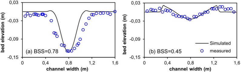
[image:5.595.45.293.399.492.2] [image:5.595.105.503.618.738.2]

centreline (±0.6 m) is set to be finer (Dy1= 0.02 m) than that in other parts (Dy2= 0.05 m). The computational mesh in the basin consists of 80116 cells. The time step for flow and sediment cal-culation is set the same at 0.009 s. The Manning’s roughness coef-ficient n in the basin is given a value of 0.03 s/[m1/3_{]. The model} was run for 2 h of experiment time. Eq.(4) is used to calculate the entrainment and deposition fluxes in this case.Fig. 6(a) shows the simulated bed change pattern around the inflow region at the

[image:6.595.59.528.68.188.2]

centre part of the basin after 4 h, andFig. 6(b) demonstrates the flow velocity field and bed shear stress. It can be seen that the inflow pipe has the biggest bed shear stress due to the high flow velocity, and the inflow pipe outfall area and the outlet area also have higher bed shear stress. Therefore, it can be seen that signif-icant erosion occurs at the outfall area due to the inflow of clear water, then the eroded sediment moves downstream and deposits forming a hill. Since only basin area is erodible, no bed changes are found at the outlet area.Fig. 7further shows the comparison of the measured and simulated bed changes along the longitudinal cen-treline at 1 h, 2 h and 4 h. All have a satisfying Brier Skill Score (BSS). Overall, the simulated morphological evolution tendency at 1 h and 2 h are in good agreement with the measured results. However, the maximum deposition heights are slightly under-predicted, with a 13.4% difference at 1 h and 30.6% at 2 h. Further-more, it can be seen that the model overestimates the erosion depth at the inlet of the basin. There the simulated erosion is much more severe than the measured erosion. This is most likely because secondary flow plays an important role here; however, these non-hydrostatic flows are neglected in the current model.

[image:6.595.50.535.447.579.2]

Fig. 5.Bed topography contour at 20 s.

Table 3

Key parameters of the case.

water depth at outlet 0.15 m inflow velocity at inlet 0.6 mm sand diameters d50= 0.6 mm

sand density 2650 kg/m3

settling velocity 0.013 m/s Manning’s coefficient 0.03 s/[m1/3

]

sediment porosity 0.35

mesh size Dx = 0.1 m,Dy1= 0.02 m,Dy2= 0.05 m

mesh number 80116 cells

(a)

(b)

Fig. 6.(a) Bed topography contour, and (b) bed shear stress and velocity field at 2h.

-0,2 -0,1 0,0 0,1 0,2

-1,00 1,00 3,00 5,00

elev

atio

n (m

)

distance downstream of dam (m) measured:1hr

simulated:1hr

-0,2 -0,1 0,0 0,1 0,2

-1,00 1,00 3,00 5,00

elev

atio

n (m

)

distance downstream of dam (m) measured:2hr

simulated:2hr

-0,2 -0,1 0,0 0,1 0,2

-1,00 1,00 3,00 5,00

elev

atio

n (m

)

distance downstream of dam (m) measured:4hr

simulated:4hr

(a) _BSS=0.79 (b) _BSS=0.89 (c) _BSS=0.90

[image:6.595.56.524.622.736.2]

3.2. Application in a stormwater pond

Stomwater ponds are characterised by urban runoff detention, runoff quality improvement and sediment trapping. The decrease in flow velocity and the low energy environment causes deposition of fine sediments delivered by urban flows as it enters the pond. Stormwater pond sedimentation leads to a decrease in pond stor-age capacity and triggers environmental and economic issues. The validated model is applied to a case study of a stormwater pond in Newcastle Great Park and based on the results, improved understanding of fine sediment dynamics is developed.

3.2.1. Study site

The study area is located in Ouseburn catchment (the black boundary in Fig. 8a) in Newcaslte upon Tyne in the UK. The stormwater pond connects the upstream newly built urban devel-opment and the Ouseburn River. Fig. 8c shows the simulated domain which is an area of 230 m by 140 m. It was observed that the pond is covered with dense vegetation which protects the local bed. For simulations, the flow discharge is input to the model via a pipe section as an upstream boundary. The other boundary is set to

be free open which means that the floodwater can freely flow out based on the local flow conditions.

3.2.2. Model scenarios

Three scenarios were considered: non-flood (5 year), sewer design (30 year) and flood (100 year) (Fig. 9a). Also, rainfall events in the extreme flow year 2012 with 15 min interval rainfall mea-surements at the Jesmond Dene gauging station (EA #19356) were used to conduct an annual sediment simulation, and the flow at the inlet for the identified rainfall events is quantified by using the physically-based conceptual rainfall-runoff model – the Revitalised Flood Hydrograph (ReFH) model (Fig. 9b).

Allen et al. (2015)measured the continuous flow records from January to May 2015 at the pond’s outfall. The ReFH rainfall runoff model is calibrated with the observed flow data sets by varying the drainage length parameter (DPLBAR) in the model. Based on the field survey, the fine sediment composes of three classes: d10 = 5mm (fine silt), d50 = 12mm (fine silt) and d90 = 50mm (silt) that were obtained from the manual sampling and equally distributed as an input in the upstream boundary. The fine sediment concen-tration is estimated based on the regression relationships between flow, turbidity and suspended sediment concentration from the analogue catchment (Ahilan et al., 2016). In order to assess the rel-ative impact of the pond on the hydrologic and morphologic responses during high flow events, two Digital Elevation Model (DEM) data sets were incorporated in the model setup. The current DEM represents existing topography (‘with’) pond condition and the DEM corresponding to the year 2000 represents the predevel-opment stage (‘without’) pond scenario in the hydro-morphodynamic model. Table 4 lists the key information about this case study.

3.3. Model validation with sampling data

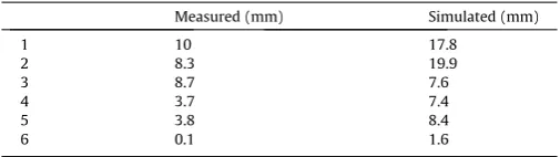
Allen et al. (2015)surveyed the cumulative sediment deposition at monthly intervals at six locations in the pond during the moni-toring period, which is used to validate the morphodynamic model in simulating sediment deposition in the pond. Flow events between 23/04/2015 and 26/05/2015 (as shown in Fig. 10) were modelled because there are a number of high flow events over the period apart from low base flows.Fig. 10shows the simulated sediment deposition in the pond and the location of the six moni-toring points. It indicates that the main deposition area is located at the outfall area. This is because the flow velocity sharply decreases after the water flows to the pond from upstream pipe, this leads to bed shear stress be so small that sediment particles settle down to the bed. Resuspension during high flows causes slight sedimentation in the far area from the outfall.Table 5shows the measured and simulated depths at the six monitoring points. It is indicated that the model predicts the sedimentation in the stormwater pond generally well despite the fact that there are

Pond coordinates: 55.024948, -1.650234

(a)

[image:7.595.52.286.319.574.2]

(b) (c)

Fig. 8.(a) Newcastle Great Park Development Site, (b) the built stormwater ponds along the river, (c) the simulated domain.

0 1 2 3 4 5

2,5

flow (m

3/s)

time (h)

5-year 30-year 100-year

0,00% 0,04% 0,08% 0,12% 0,16% 0,20%

0 0,3 0,6 0,9 1,2 1,5

0,0 0,5 1,0 1,5 2,0 23.04 28.04 04.05 09.05 15.05 20.05 26.05

SSC (

m

3/m 3)

Fl

ow

(m

3/s)

date

flow

sediment

(a)

(b)

[image:7.595.78.528.624.737.2]

clear discrepancies at some points. These differences are expected because of the uncertainty factors in reality. The main uncertainty factors include: (1) the stormwater pond is covered by a variety of soft vegetation which causes clear implication on flow dynamics and sediment transport, however, this is difficult to quantify and predict; (2) the inflow discharge and sediment concentration are quantified based on a conceptual rainfall-runoff model and regres-sion relationship between flow and turbidity, thus this brings about uncertainties in model inputs; (3) sediment particles are very fine, and the sedimentation depth is small, the field monitor-ing quantifies sediment weights rather depths which might cause some errors to quantify its real depth. Despite of the discrepancies, it can be seen that both simulated and measured shows a higher deposition near the outfall location and a smaller sedimentation at the far-point from the outfall. Therefore, considering the main objective of this study in developing better understanding of fine suspended load transport, the model results are deemed to be adequate.

3.4. Fine-grained sediment tracking during single events

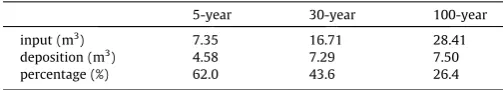
The validated model is used in the hydro-morphological simu-lations during single events (5-year flow, 30-year flow, and 100-year flow).Fig. 11shows the water depths, suspended load concen-tration, and bed shear stress and velocity field during the flow peak for each scenario, as well as the resultant sediment deposition in the stormwater pond after each event. In the viewpoint of hydro-dynamic effects, it is clear that the pond has the capability to store the 5-year flow, and the sediment particles in the flow bodies are mostly trapped in the stormwater pond (Fig. 11b) and gradually settle down in the stormwater pond because of the slow flow velocity and the low bed shear stress. However, during the 30-year and 100-30-year flow events (Fig. 11f and j), a considerable amount of water flows from the pond into the river, which trans-ports fine sediments downstream. As shown in Fig. 11f and j, although the waters in the pond still have relative higher sus-pended load, sediment particles are flushed out to the river with the increasing inflow. This leads to deposition not only inside the pond, but also in the river downstream (Fig. 11g and l).Table 6

quantifies the input sediments and the deposited sediments for the three scenarios. It shows that the increasing of inflow magni-tude results in a decrease in sediment trapping efficiency of the pond as expected.

Before building the stormwater pond, the urban flows were directly drained into the river. The simulated results inFig. 12

clearly shows that the direct drainage to the watercourse leads to much wider inundation and sedimentation during flooding in comparison with that with the ‘pond’ inFig. 12. Consequently, sed-iment particles are deposited in the inundated areas after flood recession, as demonstrated inFig. 12f and j. Even for the more fre-quent 5-year flow event, the direct drainage causes considerable amount of sedimentation in the river channel. If there is any, the contaminants attached with sediment particles will potentially influence the water quality in the receiving water. Therefore, the simulations imply that the stormwater pond has the benefits of retaining urban flows and trapping sediment particles generated from upstream urban catchment. The model is capable of quantita-tively simulating and qualitaquantita-tively assessing the performance of a stormwater pond in managing urban floods.

3.5. Fine sediment dynamics varying with flows

[image:8.595.39.541.85.244.2]

As indicated inTable 4, an extreme event in year, 2012, was simulated by the validated model in order to numerically investi-gate the fine sediment response to an extreme flood event. Table 4

The data and key parameters used in the study.

Data Description Purpose

DEMs developed bed with pond: 1 m1 m

predevelopment without pond: 1 m1 m

Model input

Sediment concentration it is estimated based on the regression relationships between flow, turbidity and suspended load concentration from the analogue catchment (Ahilan et al., 2016)

Recorded inflow 23/04/2015–26/05/2015 Model validation

Scenario-based hydrograph 5-year flow (non-flooding)30-year flow (designed flow)100-year flow (flooding)

Analysis of dynamics of flow and fine suspended sediment

2012 extreme inflow modelled hydrograph based on the measured rainfall with 15 min interval at the Jesmond Dene gauging station

Sediment composition d10 = 5mm (fine silt) d50 = 12mm (fine silt) d90 = 50mm (silt)

Model input

Sediment density 1800 kg/m3 Manning’s roughness coefficient n = 0.038 s/[m1/3

] Mesh size/number 1 m1 m/230140 cells

1

2

3

4

5

[image:8.595.59.259.275.423.2]

6

[image:8.595.32.285.474.545.2]

Fig. 10.Simulated sediment deposition in the stormwater pond.

Table 5

Measured and simulated deposition depth at the 6 monitoring points.

Measured (mm) Simulated (mm)

1 10 17.8

2 8.3 19.9

3 8.7 7.6

4 3.7 7.4

5 3.8 8.4

Fig. 13plots the inflow at the pond inlet and the cumulative sedi-ment deposition over the whole period in the study domain. Clearly, we can see a non-linear relationship between inflow charge and cumulative deposition which demonstrates two dis-tinctively different response modes: (1) steadily rising (e.g. zone 1 inFig. 13a), and (2) sharply dropping (zone 2 inFig. 13a). To look

at the trend of change in deposition volume and the inflow dis-charge inFig. 13b, we found that a high inflow leads to a sharp increase in deposition, and consistent low flows increase the sedi-mentation, but with a lower rate. However, the extreme flows in

Fig. 13b reduce the deposition volume sharply, and the higher the inflow, the more significant the reduction is.

Fig. 14further demonstrates the changes of pond sedimentation due to the three selected representative events in the year 2012 (Event 1, 2, and 3 inFig. 13). It is found that a considerable amount of sediment is trapped during Event 1, whilst the extreme Events 2 and 3 re-suspend the deposited sediment and transport them to the downstream, particularly in the area facing the pipe outlet. The behaviour is similar to the laboratory event reported in Sec-tion 3.1.3. At the pipe outlet bed shear stress is sufficiently high to cause re-suspension of sediments. The two different response

(a)

_(b)

(c)

_(d)

(f)

[image:9.595.55.552.69.550.2]

(e) (g) (h)

[image:9.595.41.293.620.665.2]

Fig. 11.Simulated water depths (a, e, i), suspended concentration (b, f, j), and bed shear stress and velocity field (c, g, k) during flow peak, as well as sedimentation in the stormwater pond (d, h, l) for the 5-year (a–c), 30-year (d–f), and 100-year (g–i) events.

Table 6

Sediment mass balance for different flood event.

5-year 30-year 100-year

input (m3

) 7.35 16.71 28.41

deposition (m3

) 4.58 7.29 7.50

modes observed during varying flow conditions raise a hypothesis, that is: sediment deposition in the pond increases with the inflow discharge, but after a critical value where there is a balance

between erosion and deposition, the bed will be eroded due to the high bed shear stress, and the erosion rate is proportional to the inflow magnitude.

(a)

(b)

(c)

(d)

(

e

)

(

f

)

[image:10.595.49.534.68.677.2]

(g)

(h)

(i)

To verify the hypothesis raised above, we picked out 24 differ-ent flow evdiffer-ents with a flow peak varying from 0.2 m3_{/s to 10 m}3_/s from the extreme year 2012, and quantified the deposition vol-ume before and after each event.Fig. 15plots the scatter points between the change in deposition volume and flow peak for each event, and the trendlines among the points. It can be seen that two trendlines are derived as postulated, and both have a good determination coefficient, R2_{, that is larger than 0.8. The} deposi-tion volume has a linear reladeposi-tion with a high determinadeposi-tion coef-ficient (0,8775) with the flow discharge. The linear relationship of erosion volume and flow discharge is also significant, but there is a clear large difference during extreme high flows (see Fig. 15). These two events with significant difference are event 2 and event 3 inFig. 14. With a similar high flow, event 2 has more sev-ere erosion than event 3. This is because thsev-ere is significant depo-sition in the pond before event 2 occurs, which allows more sediment to be re-suspended during the extreme flow of event 2. However event 3 occurs about 110 h after event 2, the depos-ited sediment available for re-suspension is clearly much less than the pre-event 2 volume. Therefore, this leads to a significant bias for the two events with similar high flow discharge. We found that there is a critical value defined as ‘balance point’ of the flow peak, and the value is approximately in a range of 1.79–1.96 m3_{/s for the studied stormwater pond. In other words,} sediment deposition in the stormwater pond increases with the inflow, and the rate is proportional to the flow peak when the flow peak is below the balance point; however, for the flow with a peak above the balance point, fine sediment particles will be re-suspended and transported downstream, and the re-suspension rate is proportional to the flow peak. Clearly, this balance point is a transition value causing bed deposition or erosion in the pond. This point provides a valuable indicator for stormwater ponds design and maintenance. Removing sediment from

stormwater ponds is needed periodically to maintain proper function and restore capacity to prevent localised flooding. Tradi-tionally machinery dredging is one option during dry conditions (United States Environmental Protection Agency, 2009)⁄⁄. How-ever, the understanding of ponds’ balance point can suggest a natural hydraulic regulation method, so saving maintenance cost, and sediments transporting to downstream can also improve the river habitat. Similar hydraulic regulation method has been used for sustainable sediment management in reservoirs (Kondolf, et al., 2014). It should be mentioned that the actual changes in sedimentation volume are also related to inflow volume in addi-tion to flow peak, because a larger flow volume means more fine sediments discharging into the pond. Nonetheless, the flow peak is the deterministic factor causing fine sediments either to be deposited in the pond or to be flushed out of the pond.

4. Conclusions

The study has developed a numerical model to track the hydro-morphological processes dominated by fine-grained suspended sediment, including the prediction of sediment concentration in flow bodies, and erosion and deposition caused by sediment trans-port. The model has been validated with three laboratory-scale test cases where suspended load plays a dominant role. The results show that the model is capable of reproducing the flow dynamics and the resultant morphological changes reasonably well. Applica-tions in real-world events are performed to further develop the process-based understanding of fine sediment activities in a stormwater pond during varying flow conditions. Findings drawn from this study include: (1) a stormwater pond can be used to attenuate flow peak and trap fine sediment particles, and the effect is more significant for flow events with a smaller flow peak; (2) a

0 2 4 6 8 10

0 20 40 60 80 100

fl

ow

rate

(m

3/s

)

deposition (m

3)

cumulative time (h) deposition

flow

0 0,5 1 1,5 2

0 10 20 30

fl

ow

rate

(m

3/s

)

deposition (m

3)

cumulative time (h)

0 2 4 6 8 10

5 15 25 35 45 55

0 200 400 600 800 1000

0 100 200 300 500 600 700 800

fl

ow

rate

(m

3/s

)

deposition (m

3)

cumulative time (h)

(a)

(b)

Event 1

Event 2

Event 3

(c)

zone 1

[image:11.595.89.517.68.349.2]

zone 2

balance point for the inflow peaks determines whether fine sedi-ments settled down or are re-suspended, and the value is deter-mined in a range of 1.79–1.96 m3/s for the studied pond; (3) the

[image:12.595.124.461.65.694.2]

above the value, the high flow event will flush away the sedimen-tation in the pond; and (4) the model is capable of quantitatively simulating and qualitatively assessing the performance of a stormwater pond in managing urban water quantity and quality.

Acknowledgements

The work is supported by the UK EPSRC Grant (No. EP/ K013661/1) and the open fund Grant (No. SKHL1607) from Sichuan University. The authors thank Environment Agency for providing rainfall, DTM and land-use data sets for the stormwater pond case study. The data associated with this paper are openly available from the University of Nottingham data repository: 10.17639/ nott.335.

References

Abad, J.D., Buscaglia, G.C., Garcia, M.H., 2008. 2D stream hydrodynamic, sediment transport and bed morphology model for engineering applications. Hydrol. Process. 22 (10), 1443–1459.

Ahilan, S., Guan, M., Sleigh, A., Wright, N., Chang, H., 2016. The influence of floodplain restoration on flow and sediment dynamics in an urban river. J. Flood Risk Manage.https://doi.org/10.1111/jfr3.12251.

Allen, D., Arthur, S., Haynes, H., Olive, V., 2017. Multiple rainfall event pollution transport by sustainable drainage systems: the fate of fine sediment pollution. Int. J. Environ. Sci. Technol. 14 (3), 639–652.

Allen, D., Olive, V., Arthur, S., Haynes, H., 2015. Urban sediment transport through an established vegetated swale: long term treatment efficiencies and deposition. Water 7 (3), 1046–1067.

Bohorquez, P., Fernandez-Feria, R., 2008. Transport of suspended sediment under the dam-break flow on an inclined plane bed of arbitrary slope. Hydrol. Process. 22 (14), 2615–2633.

Begnudelli, L., Valiani, A., Sanders, B.F., 2010. A balanced treatment of secondary currents, turbulence and dispersion in a depth-integrated hydrodynamic and bed deformation model for channel bends. Adv. Water Resour. 33 (1), 17–33. Birch, G.F., Matthai, C., Fazeli, M.S., 2006. Efficiency of a retention/detention basin to

remove contaminants from urban stromwater. Urban Water J. 3 (2), 69–77. Cao, Z., Pender, G., Wallis, S., Carling, P., 2004. Computational dam-break hydraulics

over erodible sediment bed. J. Hydraul. Eng. 130 (7), 689–703.

Costabile, P., Macchione, F., 2015. Enhancing river model set-up for 2-D dynamic flood modelling. Environ. Modell. Software 67, 89–107.

Crosa, G., Castelli, E., Gentili, G., Espa, P., 2010. Effects of suspended sediments from reservoir flushing on fish and macroinvertebrates in an alpine stream. Aquat. Sci. 72 (1), 85–95.

Dadson, S., Hall, J., Murgatroyd, A., Acreman, M., Bates, P., Beven, K., Heathwaite, L., Holden, J., Holman, I., Lane, S., O’Connell, E., Penning-Rowsell, E., Reynard, N., Sear, D., Thorne, C., Wilby, R., 2017. A restatement of the natural science

evidence concerning catchment-based ‘natural’ flood management in the United Kingdom. Proc. R. Soc. London, Ser A 473 (2199).

Duan, J.G., Nanda, S.K., 2006. Two-dimensional depth-averaged model simulation of suspended sediment concentration distribution in a groyne field. J. Hydrol. 327 (3), 426–437.

Eekhout, J.P., Hoitink, A.J., de Brouwer, J.H., Verdonschot, P.F., 2015. Morphological assessment of reconstructed lowland streams in the Netherlands. Adv. Water Resour. 81, 161–171.

United States Environmental Protection Agency, Stormwater wet pond and wetland management guidebook, February 2009, https://www3.epa.gov/npdes/pubs/ pondmgmtguide.pdf.

Guan, M., Wright, N., Sleigh, P., 2013. A robust 2D shallow water model for solving flow over complex topography using homogenous flux method. Int. J. Numer. Meth. Fluids 73 (3), 225–249.

Guan, M., Wright, N., Sleigh, P., 2014. 2D Process based morphodynamic model for flooding by non-cohesive dyke breach. J. Hydraul. Eng. 140 (7).

Guan, M., Wright, N., Sleigh, P., 2015a. Multimode morphodynamic model for sediment-laden flows and geomorphic impacts. J. Hydraul. Eng. 141 (6). Guan, M., Wright, N.G., Sleigh, P.A., Carrivick, J.L., 2015b. Assessment of

hydro-morphodynamic modelling and geomorphological impacts of a sediment-charged jökulhlaup, at Sólheimajökull, Iceland. J. Hydrol. 530, 336–349. Guertault, L., Camenen, B., Peteuil, C., Paquier, A., Faure, J.B., 2016. One-dimensional

modeling of suspended sediment dynamics in dam reservoirs. J. Hydraul. Eng. 142 (10).

Hou, J., Liang, Q., Zhang, H., Hinkelmann, R., 2015. An efficient unstructured MUSCL scheme for solving the 2D shallow water equations. Environ. Modell. Software 66, 131–152.

Hu, P., Cao, Z., 2009. Fully coupled mathematical modeling of turbidity currents over erodible bed. Adv. Water Resour. 32 (1), 1–15.

Hu, P., Cao, Z., Pender, G., Tan, G., 2012. Numerical modelling of turbidity currents in the Xiaolangdi reservoir, Yellow River, China. J. Hydrol. 464, 41–53. Jartun, M., Ottesen, R.T., Steinnes, E., Volden, T., 2008. Runoff of particle bound

pollutant from 2230 urban impervious surfaces studied by analysis of sediment from stormwater traps. Sci. Total Environ. 396 (2–3), 147–163.

Janocko, M., Cartigny, M.B.J., Nemec, W., Hansen, E.W.M., 2013. Turbidity current hydraulics and sediment deposition in erodible sinuous channels: laboratory experiments and numerical simulations. Mar. Pet. Geol. 41, 222–249. Jones, A., Stovin, V., Guymer, I., Gaskell, P., Maltby, L., 2008. Modelling temporal

variation sin the sediment concentrations in highway runoff. In: Proceedings from the 11th international conference on urban drainage, Edinburgh, UK. Kondolf, G.M., Gao, Y., Annandale, G.W., Morris, G.L., Jiang, E., Zhang, J., Cao, Y.,

Carling, P., Fu, K., Guo, Q., Hotchkiss, R., 2014. Sustainable sediment management in reservoirs and regulated rivers: experiences from five continents. Earth’s Future 2 (5), 256–280.

Liu, J., Minami, S., Otsuki, H., Liu, B., Ashida, K., 2004. Environ- mental impacts of coordinated sediment flushing. J. Hydraul. Res. 42 (5), 461–472.

Owens, P.N. et al., 2005. Fine-grained sediment in river systems: Environmental significance and management issues. River Res. Appl. 21 (7), 693–717. Saeedi, M., Daneshvar, S., Karbassi, A.R., 2004. Role of riverine sediment and

particulate matter in adsorption of heavy metals. Int. J. Environ. Sci. Technol. 1 (2), 135–140.

Simpson, G., Castelltort, S., 2006. Coupled model of surface water flow, sediment transport and morphological evolution”. Comput. Geosci. 32 (10), 1600–1614. Soulsby, R., 1997. Dynamics of Marine Sands: A Manual for Practical Applications.

Thomas Telford, London, UK.

Thuc, T., 1991. Two-dimensional morphological computations near hydraulic structures (Doctoral Dissertation). Asian Institute of Technology, Bangkok, Thailand.

Toro, E.F., 2001. Shock-Capturing Methods for Free-Surface Shallow Flows 326 pp., John Wiley &Sons, LTD.

Vacondio, R., Dal Palù, A., Mignosa, P., 2014. GPU-enhanced Finite Volume Shallow Water solver for fast flood simulations. Environ. Modell. Software 57, 60–75. van Rijn, L.C., 1980. Computation of siltation in dredged trench, Report No. 1267-V,

Delft Hydraulic Laboratory, Delft, The Netherlands.

Van Rijn, L.C., 1984. Sediment transport part II, suspended load transport. J. Hydraul. Eng.-ASCE 110 (11), 1613–1641.

Vörömarty, C.J., Meybeck, M., Fekete, B., Sharma, K., Green, P., Syvitski, J.P.M., 2003. Anthropogenic sediment retention: major global impacts from registered river impoundments. Global Planet. Change 39, 169–190.

Wood, P.J., Armitage, P.D., 1997. Biological effects of fine sediment in the lotic environment. Environ. Manage. 21 (2), 203–217.

Wu, W., 2004. Depth-averaged two-dimensional numerical modeling of unsteady flow and nonuniform sediment transport in open channels. J. Hydraul. Eng.-ASCE 130 (10), 1013–1024.

Xia, J., Lin, B., Falconer, R.A., Wang, G., 2010. Modelling dam-break flows over mobile beds using a 2D coupled approach. Adv. Water Resour. 33, 171–183. Zech, Y., Soares-Frazao, S., Spinewine, B., Grelle, N.L., 2008. Dam- break induced

sediment movement: Experimental approaches and numerical modelling. J. Hydraul. Res. 46 (2), 176–190.

R² = 0,8775

R² = 0,8332

-50 -40 -30 -20 -10 0 10

0 2 4 6 8 10

change in vol

u

m

e

(m

3

)

flow peak (m

3

_/s)

deposition

[image:13.595.71.263.67.232.2]

erosion