This is a repository copy of Vertex elimination orderings for hereditary graph classes.
White Rose Research Online URL for this paper:
http://eprints.whiterose.ac.uk/78858/
Version: Accepted Version
Article:
Aboulker, P, Charbit, P, Trotignon, N et al. (1 more author) (2015) Vertex elimination
orderings for hereditary graph classes. Discrete Mathematics, 338 (5). 825 - 834. ISSN
0012-365X
https://doi.org/10.1016/j.disc.2014.12.014
© 2015, Elsevier. Licensed under the Creative Commons
Attribution-NonCommercial-NoDerivatives 4.0 International
http://creativecommons.org/licenses/by-nc-nd/4.0/
Reuse
Unless indicated otherwise, fulltext items are protected by copyright with all rights reserved. The copyright exception in section 29 of the Copyright, Designs and Patents Act 1988 allows the making of a single copy solely for the purpose of non-commercial research or private study within the limits of fair dealing. The publisher or other rights-holder may allow further reproduction and re-use of this version - refer to the White Rose Research Online record for this item. Where records identify the publisher as the copyright holder, users can verify any specific terms of use on the publisher’s website.
Takedown
If you consider content in White Rose Research Online to be in breach of UK law, please notify us by
promoting access to White Rose research papers
White Rose Research Online
Universities of Leeds, Sheffield and York
http://eprints.whiterose.ac.uk/
This is an author produced version of a paper accepted for publication in
Discrete Mathematics
White Rose Research Online URL for this paper:
http://eprints.whiterose.ac.uk/id/eprint/78858
Paper:
Vertex elimination orderings for hereditary graph
classes
Pierre Aboulker∗, Pierre Charbit∗, Nicolas Trotignon† and Kristina Vuˇskovi´c‡
February 16, 2014
AMS Classification: 05C75
Abstract
We provide a general method to prove the existence and compute efficiently elimination orderings in graphs. Our method relies on sev-eral tools that were known before, but that were not put together so far: the algorithm LexBFS due to Rose, Tarjan and Lueker, one of its properties discovered by Berry and Bordat, and a local decomposition property of graphs discovered by Maffray, Trotignon and Vuˇskovi´c.
1
Introduction
In this paper all graphs are finite and simple. A graph Gcontains a graph F if F is isomorphic to an induced subgraph of G. A class of graphs is
∗Universit´e Paris 7 – Paris Diderot, LIAFA, email: pierre.aboulker@liafa.jussieu.fr,
pierre.charbit@liafa.jussieu.fr
†CNRS, LIP, ENS Lyon, UCBL, Universit´e de Lyon, INRIA email:
nicolas.trotignon@ens-lyon.fr. Partially supported by the French Agence Nationale de la Recherche under referenceANR-13-BS02-0007.
‡School of Computing, University of Leeds, Leeds LS2 9JT, UK, and Faculty of
Com-puter Science (RAF), Union University, Knez Mihajlova 6/VI, 11000 Belgrade, Serbia. email: k.vuskovic@leeds.ac.uk. Partially supported by EPSRC grant EP/K016423/1 and Serbian Ministry of Education and Science projects 174033 and III44006.
The authors are also supported by PHC Pavle Savi´c grant, jointly awarded by EGIDE, an agency of the French Minist`ere des Affaires ´etrang`eres et europ´eennes, and Serbian Ministry of Education and Science.
The first, second and fourth authors are partially supported by the French Agence Na-tionale de la Recherche under referenceanr-10-jcjc-Heredia.
hereditary if for every graph G of the class, all induced subgraphs of G belong to the class. A graphG is F-free if it does not contain F. WhenF
is a set of graphs,G isF-freeif it is F-free for every F ∈ F. Clearly every hereditary class of graphs is equal to the class of F-free graphs for someF
(F can be chosen to be the set of all graphs not in the class but all induced subgraphs of which are in the class). The induced subgraph relation is not a well quasi order (contrary for example to the minor relation), so the set
F does not need to be finite.
When X ⊆V(G), we write G[X] for the subgraph of G induced byX. An ordering (v1, . . . , vn) of the vertices of a graph G is an F-elimination
ordering if for every i= 1, . . . , n,NG[{v1,...,vi}](vi) is F-free. Note that this
is equivalent to the existence, in every induced subgraph of G, of a vertex whose neighborhood isF-free.
Let us illustrate our terminology on a classical example. We denote by S2 the independent graph on two vertices. A vertex is simplicial if its neighborhood isS2-free, or equivalently is a clique. A graph ischordal if it is hole-free, where a holeis a chordless cycle of length at least 4.
Theorem 1.1 (Dirac [12]) Every chordal graph admits an {S2}
-elimination ordering.
Theorem 1.2 (Rose, Tarjan and Lueker [26]) There exists a
linear-time algorithm that computes an {S2}-elimination ordering of an input
chordal graph.
Motivation, goals, and outline of the paper
We believe that elimination orderings are important, because several classi-cal hereditary classes, such as perfect graphs or even-hole-free graphs, admit deep decomposition theorems that are hard to use for algorithmic purposes. For more details, we send the reader to surveys ([31] for perfect graphs and [33] for even-hole-free graphs). Sometimes, as we shall see, the existence of a vertex with some local structural property is more useful for the design of efficient algorithms than a global description of the class. Even for chordal graphs that are rather well structured, elimination orderings are the basis for the fastest algorithms.
1. LexBFS, a classical algorithm discovered by Rose, Tarjan and Lueker [26], and some of its properties discovered by Berry and Bor-dat [3].
2. A local decomposition property of graphs discovered by Maffray, Trotignon and Vuˇskovi´c [23]. This property is called Property (⋆)
in [23], but here we give it a more meaningful name oflocal decompos-ability.
In Section 2, we explain the first ingredient, and in Section 3 the sec-ond. We conclude Section 3 by illustrating how our method reproduces the classical proofs of Theorems 1.1 and 1.2, so that we may consider the rest of our work as a generalization of these.
In Section 4 we give two classes of graphs for which the existence of an F-elimination ordering is proved in previous works (namely even-hole-free graphs and square-theta-even-hole-free Berge graphs). We explain for each of them how our method can be used prove the existence of the ordering. For even-hole-free graphs, our method leads to speeding up the algorithm that computes a maximum clique. To be more specific, it turns out that the classes in Section 4 are slight generalizations of even-hole-free graphs and square-theta-free Berge graphs, defined by excluding different Truemper configurations, that are special types of graphs (defined formally at the end of this section) that play an important role in the study of hereditary graph classes (see survey [34]). This fact is interesting to us, especially because Truemper configurations appear also in the following section.
In Section 5, we apply systematically our method to produce classes of graphs that admit F-elimination orderings for all possible non-empty sets of graphsF made of non-complete graphs on three vertices (there are seven such setsF). This leads us to define seven classes of graphs, each of which having its own elimination ordering by our method. Two of these classes were previously studied (namely universally signable graphs and wheel-free graphs) and five of them are new. For almost all these classes, we get something from the ordering: a bound on the chromatic number, a coloring algorithm, or an algorithm for the maximum clique problem. To our great surprise, this systematic application of the method outlined in this paper leads again to classes that are all defined by excluding some Truemper con-figurations.
Section 6 is devoted to open questions.
• Maximum weighted clique in even-hole-free graphs in timeO(nm).
• Maximum weighted clique in universally signable graphs in timeO(n+ m).
• Coloring in universally signable graphs in time O(n+m).
Terminology and notation
Forx ∈V(G), N(x) denotes the set of neighbors of x, and N[x] = N(x)∪ {x}. For a set of vertices S,N(S) denotes the set of vertices not inS that have a neighbor in S, and N[S] = S∪N(S). For S ⊆V(G), G[S] denotes the subgraph of Ginduced by S, and G−S =G[V(G)−S].
Recall that a hole in a graph is a chordless cycle of length at least 4, where thelength of a hole is the number of its edges. A hole is evenorodd
according to the parity of its length.
Sometimes, we consider weighted graphs, which are graphs given with a non-negative weight for every vertex. The weight of a subset of vertices is then the sum of the weights of its elements. The usual problem of finding a maximum clique generalizes to weighted graphs to the problem of finding a clique of maximum weight.
In all complexity analysis of the algorithms, n denotes the number of vertices of the input graph, and m the number of edges. We say that an algorithm runs inlinear time if its complexity is O(n+m).
Truemper configurations
Special types of graphs that are called Truemper configurations appear in different sections of this work, so let us define them now. A3-path
configu-rationis a graph induced by three internally vertex disjoint paths of length
at least 1, P1 =x1. . . y1,P2 =x2. . . y2 and P3 =x3. . . y3, such that either x1 =x2 =x3 orx1, x2, x3 are all distinct and pairwise adjacent, and either y1=y2=y3ory1, y2, y3are all distinct and pairwise adjacent. Furthermore, the vertices ofPi∪Pj,i6=j, induce a hole. Note that this last condition in the definition implies the following.
• Ifx1, x2, x3are distinct (and therefore pairwise adjacent) andy1, y2, y3 are distinct, then the three paths have length at least 1. In this case, the configuration is called aprism.
Figure 1: Pyramid, prism, theta and wheel (dashed lines represent paths)
formed by the two other paths). In this case, the configuration is called atheta.
• Ifx1 =x2 =x3 and y1, y2, y3 are distinct, or if x1, x2, x3 are distinct and y1 =y2 = y3, then at most one of the three paths has length 1, and the others have length at least 2. In this case, the configuration is called apyramid.
A wheel (H, v) is a graph formed by a hole H, called the rim, and a
vertexv, called the center, such that the center has at least three neighbors on the rim. A Truemper configuration is a graph that is either a prism, a theta, a pyramid or a wheel (see Figure 1).
2
A theorem on LexBFS orderings
LexBFS is a linear time algorithm of Rose, Tarjan and Lueker [26] whose input is any graphGtogether with a vertexs, and whose output is a linear ordering of the vertices ofG starting ats. A linear ordering of the vertices of a graph Gis aLexBFS ordering if there exists a vertexs ofG such that the ordering can be produced by LexBFS when the input is G, s. As the reader will soon see, we do not need to define LexBFS more precisely. The purpose of this section is to provide an alternative proof of the following result.
Theorem 2.1 (Berry and Bordat [3]) IfGis a non-complete graph and
zis the last vertex of a LexBFS ordering of G, then there exists a connected
componentC of G−N[z]such that for every neighborxof z, either N[x] =
N[z], or N(x)∩C 6=∅.
is stated in term of moplexes in [3]. We find it more convenient for our purpose to state it as we do. We now give an alternative proof of Theorem 2.1 for several reasons. First, it is shorter than the original proof mainly because it relies on the following nice characterization of LexBFS orderings instead of the full description of the algorithm. Second, we believe that Lemma 2.3 that we use in our proof and that was not stated explicitly before is of independent interest.
Theorem 2.2 (Brandst¨adt, Dragan and Nicolai [4]) An ordering ≺
of the vertices of a graph G = (V, E) is a LexBFS ordering if and only
if it satisfies the following property: for all a, b, c∈V such that c ≺b≺a,
ca∈E andcb /∈E, there exists a vertex dinGsuch that d≺c, db∈E and
da6∈E.
Let us strengthen a little this property for our purposes.
Lemma 2.3 Let ≺ be a LexBFS ordering of a graph G = (V, E). Let z
denote the last vertex in this ordering. Then for all verticesa, b, c∈V such
that c ≺b ≺ a and ca∈ E, there exists a path from b to c whose internal
vertices are disjoint fromN[z].
proof — By contradiction assume there exists such a triple c ≺ b ≺ a for which no such path exists fromb toc. Choose this triple to be minimal with respect to the sum of the positions of its elements in the ordering. Observe that since b cannot be adjacent to c, by Theorem 2.2 there is a vertexdsuch that d≺c,db∈E andda6∈E. There must be a pathP from c to d whose internal vertices are disjoint from N[z] otherwise d ≺ c ≺ b would contradict the minimality of c ≺b ≺ a. Since db ∈E, d must be a neighbor of z otherwise P ∪ {d} is a path that contradicts the hypothesis. In particular, z6=a. So we can apply Theorem 2.2 to the triple d≺a≺z. Thus there is a vertexesuch thate≺d,ea∈E and ez /∈E. But again by minimality of c ≺ b ≺a, there exist two paths, one from e to c (from the triple e ≺ c ≺ a), and one from e to b (from the triple e ≺ b ≺ a) whose internal vertices are disjoint fromN[z]. Since eis a non-neighbor of z, the union of these paths contains a path frombtocwhose internal vertices are disjoint from N[z], a contradiction. 2
With this lemma, we are now able to easily prove the aforementioned theorem.
Let x be a neighbor of z, and assume that N(x) ⊆ N[z]. To show that in this case N[x] =N[z], let y be another neighbor of z, and assume xy /∈ E(G). Either x ≺ y or y ≺ x, but in both cases, Lemma 2.3 with a= z implies the existence of a neighbor of x that is not a neighbor of z, contradicting the assumption.
Now assume that N(x) 6⊆N[z]. Denote by u the last vertex in ≺ that does not belong to N[z], and by C the connected component of G−N[z] containingu. We now show thatCis the desired component. Ifx≺u, then by Lemma 2.3 applied tox ≺u≺z, there exists a path from x tou which does not meet N[z], so x must have a neighbor in C. So we may assume that u ≺x and that u is not adjacent to x. Since x has a neighboru′ not belonging to N[z], we must have u′ ≺ u. Now by Lemma 2.3 applied to u′ ≺u≺x,uand u′ belong to the same componentC. 2
3
Locally
F
-decomposable graphs
Let F be a set of graphs. We are interested in graphs G that admit F -elimination orderings (which is equivalent to say that every induced sub-graph of G has a vertex whose neighborhood is F-free). A much stronger property is the one of being locally F-free : every vertex of Ghas a F-free neighborhood. The following property, that sits between these two, was in-troduced by Maffray, Trotignon and Vuˇskovi´c in [23] (where it was called Property (⋆)).
Definition 3.1 Let F be a set of graphs. A graph G is locally F -decomposable if for every vertex v of G, every F ∈ F contained in N(v)
and every connected componentC ofG−N[v], there existsy∈F such that
y has a non-neighbor in F and no neighbors in C.
A class of graphs C is locally F-decomposable if every graph G ∈ C is
locallyF-decomposable.
It is easy to see that if a graph is locally F-decomposable, then so are all its induced subgraphs. Therefore, for all sets of graphs F, the class of graphs that are locallyF-decomposable is hereditary.
Observe that a complete graph is locally F-decomposable for any set of graphs F. On the other hand, a complete graph may fail to have an
Here is now our main result. A similar theorem was given in [23] with another kind of ordering (not worth defining here) instead of LexBFS. This ordering was also lexicographic in some sense, but it could not be computed in linear time.
Theorem 3.2 If F is a set of non-complete graphs, and G is a locally F
-decomposable graph, then every LexBFS ordering of G is an F-elimination
ordering.
proof — Let z be the last vertex of a LexBFS ordering of G. If G is complete, thenN(z) isF-free because no graph ofFis complete. Otherwise, the connected componentC given by Theorem 2.1 is such that every vertex ofN(z) that has non-neighbors inN(z) has a neighbor inC. So by definition of localF-decomposability, N(z) must be F-free.
Therefore, any LexBFS ordering is an F-elimination ordering, because if (v1, v2, . . . , vn) is a LexBFS ordering, then for all i, (v1, v2, . . . , vi) is a LexBFS ordering of G[{v1, v2, . . . , vi}] (this follows for instance from the characterization of LexBFS orderings given in Theorem 2.2). 2
Let us now illustrate how Theorem 3.2 can be used with the simplest possible set made of non-complete graphs: F ={S2}, whereS2 is the inde-pendent graph on two vertices. The following is of course well known, but we write its proof to illustrate our notions.
Lemma 3.3 A graph G is locally {S2}-decomposable if and only if G is
chordal.
proof — Suppose G is not locally {S2}-decomposable. Then for some
x∈V(G) and some connected componentC ofG−N[x],G[N(x)] contains an induced subgraph F isomorphic to S2, and every vertex of F has a neighbor inC. This clearly implies thatG contains a hole.
To prove the converse, suppose thatGcontains a holeH, and lety, x, z be three consecutive vertices of H. Let C be the connected component of G−N[x] that contains the vertices of H − {x, y, z}. Then {y, z} is an S2 ofN(x), and bothy and zhave neighbors in C. Therefore,Gis not locally
{S2}-decomposable. 2
4
Even-hole-free graphs and perfect graphs
In this section, we show how local decomposability can be used to provide elimination orderings and algorithms for even-hole-free graphs and some Berge graphs. A graphGisBerge ifGand Gare odd-hole-free. In the last few decades much research was devoted to the study of Berge graphs, odd-hole-free graphs and even-odd-hole-free graphs (for surveys see [31, 33]). For all these classes global decomposition theorems are known. Most famously the celebrated proof of the Strong Perfect Graph Conjecture (which states that
a graph is perfect if and only if it is Berge) obtained in 2002 by Chudnovsky,
Robertson, Seymour and Thomas [7] is based on a decomposition theorem for Berge graphs. Also decomposition theorems were obtained for even-hole-free graphs [10], the most precise one by da Silva and Vuˇskovi´c [29]. Unfortunately, up to now, no one knows how these decomposition theorems can be used to design fast algorithms for optimization problems.
The results that we present here are in fact proved for generalizations of Berge graphs and even-hole-free graphs, the so-calledsigned graphs. We want to state their definitions here, because we find it interesting that they make use of the same kind of obstructions as the classes of graphs in the next section. A graph is odd-signable if there exists an assignment of 0,1 weights to its edges that makes every chordless cycle of odd weight. A graph
iseven-signableif there exists an assignment of 0,1 weights to its edges that
makes every triangle of odd weight and every hole of even weight. In [32] Truemper proved a theorem that characterizes graphs whose edges can be assigned 0,1 weights so that chordless cycles have prescribed parities. The characterization states that this can be done for a graphG if and only if it can be done for all Truemper configurations and K4’s contained in G. An easy consequence of this theorem when applied to odd-signable and even-signable graphs gives the following characterizations of these classes (see [11]). Asector of a wheel is a subpath of the rim of length at least 1 whose ends are adjacent to the center and whose internal vertices are not. A wheel is even if it has an even number of sectors, and it is odd if it has an odd number of sectors of length 1.
• A graph isodd-signable if and only if it is{theta, prism, even wheel} -free.
• A graph iseven-signable if and only if it is{pyramid, odd wheel}-free.
[28] and [23]), and were obtained by a special kind of lexicographic ordering of the vertices that is different from LexBFS (but more closely related to decomposition). Proving the existence of the ordering directly from The-orem 3.2 allows in both cases for the desired ordering to be computed in linear-time. A 4-hole is a hole of length 4.
Theorem 4.1 (da Silva and Vuˇskovi´c [28]) 4-hole-free odd-signable graphs are locally hole-decomposable.
Theorems 4.1 and 3.2 directly imply that 4-hole-free odd-signable graphs admit a hole-elimination ordering. Theorem 4.1 is used in [28] to obtain a robust O(n2m)-time algorithm for computing a maximum weighted clique in a 4-hole-free odd-signable graph (and hence in an even-hole-free graph). We now show how to reduce this complexity to O(nm).
Theorem 4.2 There is anO(nm)-time algorithm whose input is a weighted
graphGand whose output is a maximum weighted clique of Gor a certificate
proving thatG is not 4-hole-free odd-signable.
proof — Let H denote the class of all holes and consider the following algorithm. Compute in linear time a LexBFS ordering (v1, . . . , vn) ofG. By Theorems 3.2 and 4.1, this ordering is an H-elimination ordering if G is a 4-hole-free odd-signable graph. Testing whether a graph is chordal can be done in linear time [26], and hence it can be checked inO(nm)-time whether (v1, . . . , vn) is anH-elimination ordering.
So, we may assume that (v1, . . . , vn) is an H-elimination ordering of G. We suppose inductively that a maximum weighted clique of G[{v1, . . . , vn−1}] is found in time O((n− 1)m). A maximum weighted clique of G[N[vn]] can be found in time O(m) [26]. So, we now know a maximum weighted clique of G[N[vn]] and a maximum weighted clique of G[{v1, . . . , vn−1}]. A maximum weighted clique among these is a maximum weighted clique ofG. All this takes time O((n−1)m) +O(m) =O(nm). 2
We now turn our attention to Berge graphs (or more precisely to even-signable graphs that generalize them). Asquare-theta is a theta that con-tains a 4-hole. Along hole is a hole of length at least 5.
Theorem 4.3 (Maffray, Trotignon and Vuˇskovi´c [23]) Square-theta-free even-signable graphs are locally long-hole-decomposable.
Theo-rem 4.3 an O(n7)-time robust algorithm is given in [23] for computing a maximum weighted clique in a square-theta-free Berge graph (note that this class generalizes both 4-hole-free Berge graphs and claw-free Berge graphs). It relies on a long-hole-elimination ordering. With the machinery presented here, we can obtain this ordering in linear time, but unfortunately, this does not improve the overall complexity of the maximum clique algorithm.
5
Seven generalizations of chordal graphs
In this section we apply systematically our method to all possible sets made of non-complete graphs of order 3. This leads to seven classes of graphs, two of which were studied before (namely universally signable graphs and wheel-free graphs).
To describe the classes of graphs that we obtain, we need to be more specific about wheels. A wheel is a 1-wheel if for some consecutive vertices x, y, z of the rim, the center is adjacent to y and non-adjacent to x and z. A wheel is a2-wheel if for some consecutive vertices x, y, z of the rim, the center is adjacent toxandy, and non-adjacent toz. A wheel is a3-wheel if for some consecutive verticesx, y, z of the rim, the center is adjacent to x, y and z. Observe that a wheel can be simultaneously a 1-wheel, a 2-wheel and a 3-wheel. On the other hand, every wheel is a 1-wheel, a 2-wheel or a 3-wheel. Also, any 3-wheel is either a 2-wheel or auniversal wheel (that is a wheel whose center is adjacent to all vertices of the rim).
Up to isomorphism, there are four graphs on three vertices, and three of them are not complete. These three graphs (namely the independent graph on three vertices denoted byS3, the path of length 2 denoted by P3 and its complement denoted by P3) are studied in the next lemma.
Lemma 5.1 For a graph G the following hold.
(i) G is locally {S3}-decomposable if and only if G is {1-wheel, theta,
pyramid}-free.
(ii) Gis locally {P3}-decomposable if and only ifG is 3-wheel-free.
(iii) G is locally {P3}-decomposable if and only if G is {2-wheel, prism,
pyramid}-free.
S3,{x, y, z} ⊆N(v), and H′ =H− {v, x, y, z} is a connected subgraph of G−N[v] such that every vertex of{x, y, z} has a neighbor inH′.
To prove the converse, let v ∈V(G) be such that G[N(v)] containsS3, andC a component ofG−N[v] such that every vertex ofS3 has a neighbor inC. Denote byx, y, z the three members ofS3. LetP be a chordless path from x to y with interior in C. Let Q be a chordless path from z to z′, such that V(Q)− {z} ⊆ C, z′ has neighbors in the interior of P, and is of minimum length among such paths (possibly, Q=z=z′).
Suppose that at least one ofxoryhas neighbors inQ(this implies that Qhas length at least 1). Call w the vertex of Q closest toz along Q, that has neighbors in {x, y}, and suppose up to symmetry that w is adjacent to y. Call w′ the vertex of Q closest to z along Q that has neighbors in P −y. Call x′ the neighbor of w′ in P, closest to x along P. Now, V(xP x′)∪V(zQw′)∪ {v, y}induces a theta or a 1-wheel centered at y.
Therefore, we may assume that none of x, y has a neighbor in Q. If z′ has a unique neighbor in P, then V(P)∪V(Q)∪ {v}induces a theta. If z′ has exactly two neighbors in P that are adjacent, then V(P)∪V(Q)∪ {v}
induces a pyramid. Otherwise, V(P)∪V(Q)∪ {v} contains a theta.
To prove (ii), first observe that if G contains a 3-wheel H, then H contains vertices v, x, y, z such that x, y, z is a P3, {x, y, z} ⊆ N(v), and H′=H− {v, x, y, z}is a connected subgraph ofG−N[v] such that bothx and z have a neighbor in H′. To prove the converse, let v ∈V(G) be such thatG[N(v)] contains a chordless pathxyz, andC a component ofG−N[v] such that x and z both have a neighbor in C. Then clearlyC∪ {v, x, y, z}
contains a 3-wheel.
To prove (iii), first observe that if Gcontains a 2-wheel, prism or pyra-mid H, then H contains vertices v, x, y, z such that {x, y, z} induces a P3,
{x, y, z} ⊆ N(v), and H′ = H − {v, x, y, z} is a connected subgraph of G−N[v] such that every vertex of{x, y, z} has a neighbor inH′.
To prove the converse, let v ∈V(G) be such that G[N(v)] contains P3, andC a component ofG−N[v] such that every vertex of P3 has a neighbor in C. Denote by x, y, z the vertices of P3 in such a way that xy is the only edge of G[{x, y, z}]. Let P be a path from x to y with interior in C whose unique chord is xy. Let Q be a chordless path from z to z′, such thatV(Q)− {z} ⊆C,z′ has neighbors in the interiorP, and is of minimum length among such paths (possibly,Q=z=z′).
symmetry thatwis adjacent to y. Callw′ the vertex ofQclosest tozalong Qthat has neighbors in P−y. Callx′ the neighbor of w′ inP, closest tox alongP. Now,V(xP x′)∪V(zQw′)∪ {v, y}induces a 2-wheel centered at y. Therefore, we may assume that none of x, y has a neighbor in Q. If z′ has a unique neighbor in P, then V(P)∪V(Q)∪ {v} induces a pyramid or a 2-wheel (when P has length 2). If z′ has exactly two neighbors in P that are adjacent, then V(P)∪V(Q)∪ {v} induces a prism. Otherwise, V(P)∪V(Q)∪ {v} contains a pyramid. 2
The next lemma allows us to combine the results of the previous one.
Lemma 5.2 Let F,F′,H,H′ be sets of graphs such that F and F′ contain
only non-complete graphs. Suppose that the class of locally F-decomposable
graphs is equal to the class ofH-free graphs, and that the class of locallyF′
-decomposable graphs is equal to the class of H′-free graphs. Then, the class
of locally(F ∪F′)-decomposable graphs is is equal to the class of(H∪H′)-free
graphs.
proof — Suppose thatGis locally (F ∪ F′)-decomposable. From the def-inition of local decomposability, it follows thatGis locallyF-decomposable and locally F′-decomposable. Hence, G is both H-free and H′-free. It is therefore (H ∪ H′)-free.
Suppose conversely that G is (H ∪ H′)-free. Then G is H-free and H′ -free. It is therefore locally F-decomposable and locally F′-decomposable. From the definition of local decomposability, it follows that G is locally
(F ∪ F′)-decomposable. 2
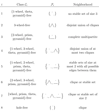
Table 1 describes eight different classes of graphs C1, . . . ,C8, all defined by excluding induced subgraphs described in the second column of the table (one of them is the class of chordal graphs that we put back to have a complete picture). The third column describes a classFi. The last column describes the class of Fi-free graphs. Inclusions between our classes and several known classes are represented in Figure 2 (where thediamond is the graph obtained from K4 by removing one edge, a cap is a cycle of length at least 5 with a unique chord joining two vertices at distance 2 on the cycle, a d-hole is 3-wheel such that the center has degree 3, and the claw
is K1,3). Observe that a d-hole is also a 2-wheel. The following theorem follows directly from Lemmas 5.1, 5.2 and 3.3.
i Class Ci Fi Neighborhood
1 {1-wheel, theta, pyramid}-free
no stable set of size 3
2 3-wheel-free
disjoint union of cliques
3 {2-wheel, prism, pyramid}-free
complete multipartite
4 {1-wheel, 3-wheel, theta, pyramid}-free
n
,
o disjoint union of at
most two cliques
5
{1-wheel, 2-wheel, prism, theta, pyramid}-free
n
,
o stable sets of size at
most 2 with all possible edges between them
6 {2-wheel, 3-wheel, prism, pyramid}-free
n
,
o
clique or stable set
7 {wheel, prism, theta, pyramid}-free
n
, ,
o clique or stable set of
size 2
8 hole-free
[image:16.612.129.478.181.570.2]clique
C7
C1
C3
C2
C5
C6
C4
C8
claw-free
[image:17.612.157.458.127.340.2]diamond-free triangle-free {d-hole, cap}-free
Figure 2: Inclusion for several classes of graphs. An arrow from A to B means “A is contained in B”. Arrows arising from transitivity are not represented.
Table 1. For i = 1, . . . ,8, the class Ci is exactly the class of locally Fi
-decomposable graphs.
With Theorem 3.2, this directly implies the following.
Theorem 5.4 For i = 1, . . . ,8, let Ci and Fi be the classes defined as in
Table 1. Then every LexBFS ordering of a graph of Ci is an Fi-elimination
ordering.
Known classes
outputs the ordering that does not rely on global decomposition. In the next subsection, we study several algorithmic consequences.
Theorem 5.5 (Conforti, Cornu´ejols, Kapoor and Vuˇskovi´c [9])
Every non-empty universally signable graph contains a simplicial vertex or
a vertex of degree2.
The second class that was studied previously is the class of wheel-free graphs and its super-classC2. These might have interesting structural prop-erties, as suggested by several subclasses, see [1] for example for a list of them. The next theorem (which follows from Theorem 5.4 fori= 2) states the only non-trivial property that is known to be satisfied by all wheel-free graphs. The original proof (due to Chudnovsky who communicated it to us but did not publish it) is by induction, and the proof relying on our method is much shorter.
Theorem 5.6 (Chudnovsky [5]) Every non-empty 3-wheel-free graph contains a vertex whose neighborhood is a disjoint union of cliques.
The following corollary extends a well-known fact: a chordal graph G has at mostnmaximal cliques.
Corollary 5.7 A 3-wheel-free graphG has at mostm maximal cliques.
proof — Induction on m. By Theorem 5.6, consider a vertex v of de-gree dwhose neighborhood is a disjoint union of cliques. By the induction hypothesis, G−v has at most m−d maximal cliques, and because of its neighborhhood,v is in at most dmaximal cliques. 2
Consequences
Table 2 describes several properties of the classes defined in Table 1. We indicate a reference for the properties that are already known, or follow easily from the given references. Let us now explain and prove all these properties.
i χ-bounded Max clique Coloring
1 f(x) =O(x2/logx) NP-hard [25] NP-hard [18]
2 No [35] O(nm) [26] NP-hard [22]
3 No [35] O(nm) NP-hard [22]
4 f(x) = 2x−1 O(n+m) ?
5 f(x) = 2x−1 O(nm) ?
6 No [35] O(n+m) NP-hard [22]
7 f(x) = max(3, x) [9] O(n+m) O(n+m)
[image:19.612.166.450.128.313.2]8 f(x) =x [12] O(n+m) [26] O(n+m) [26]
Table 2: Several properties of classes defined in Table 1
smallest known function proving so. ClassesC2,C3 andC6are notχ-bounded because they contain all triangle-free graphs, and these may have arbitrarily large chromatic number as first shown by Zykov [35]. For classesC1,C4 and
C5, we may rely on degeneracy. Say that a hereditary class of graphs is
ω-degenerate if there exists a functiongsuch that every non-empty graph in
the class has a vertex of degree at mostg(ω(G)). It is easy to check that by the greedy coloring algorithm, if a hereditary class of graphs isω-degenerate with a non-decreasing functiong, then it isχ-bounded with functiong+ 1. The function given for classes C4 and C5 follows from the fact that these classes are clearly ω-degenerate with function g(x) = 2x−2. For the class
C1, we use Ramsey theory. Kim [19] proved that for some constant c, every graph on ct2/logt vertices admits a stable set of size 3 or a clique of size t. Therefore, the vertex whose neighborhood is S3-free in any graph in C1 proves that C1 isω-degenerate with function g(x) =O(x2/logx). Observe that the results in this paragraph just improve bounds. Indeed, a theorem due to K¨uhn and Osthus [21] proves that theta-free graphs (and therefore graphs in C1,C4 andC5) areω-degenerate, but their function is quite big.
comple-ment, it is NP-hard to compute a maximum clique in anS3-free graph, and therefore in graphs from C1. Finding a maximum weighted clique in C2 is easy as follows: for every vertex v, look for a maximum weighted clique in N(v), and choose the best clique among these. This can be implemented by running n times the O(n+m) algorithm of Rose, Tarjan and Lueker, because N(v) is chordal for every v. In fact, this algorithm works in the larger class of universal-wheel-free graphs.
For C4, we need to be careful about the complexity analysis. Here is an algorithm that finds a maximum (weighted) clique in G ∈ C4. First by Theorem 5.4, we find in linear time an{S3, P3}-elimination ordering of G, say (v1, . . . , vn). This means that in G[{v1, . . . , vi}], N(vi) is a disjoint union of at most two cliques. We now show that, having this ordering, we can compute a maximum clique in time O(m). We may assume that G is connected (otherwise we work on components separately), so m ≥ n−1. Suppose inductively that a maximum clique ofG[{v1, . . . , vn−1}] is found in time O(m−d(vn)). We now take the vertices of N(vn) one by one. We give namex and label X to the first one, and check whether the next ones are adjacent to x. If so, we give them label X. If some are not adjacent tox, we give namey and label Y to the first one that we meet. The next vertices receive label X orY according to their adjacency to x ory. Note that exactly one of these adjacencies must occur, sinceN(vn) is the union of at most two cliques. At the end of this loop, the vertices with labelX and Y form at most two cliques inN(vn). They are identified in timeO(d(vn)). So, we now know all the maximal cliques ofG[N[vn]] and a maximum clique ofG[{v1, . . . , vn−1}]. A maximum clique among these is a maximum clique of G. All this takes time O(m−d(vn)) +O(d(vn)) =O(m). Observe that this algorithm relies on a constant time checking of the adjacency, so it needs the graph to be represented by an adjacency matrix. Therefore, the time complexity isO(n+m), but the space complexity is O(n2). Observe also that this algorithm is not robust. If the input graph is not in C4, the output is a set of vertices, and if it is a clique, we cannot be sure that it has maximum weight. Since C7 is a subclass of C4, we obtain an algorithm for the maximum clique problem for universally signable graphs that is faster than theO(nm)-time algorithm that follows from [9].
For classC6, the algorithm is similar to the previous one. We have to find a maximum clique in N(vn) in time O(d(vn)). It is easy to verify quickly whether the neighborhood ofvnis a clique or a stable set, and in both cases, it is immediate to find in time O(d(vn)) a maximum weighted clique in it. We omit further details.
ex-cept that we rely on a{P3}-elimination ordering ofGinstead of an{S3, P3} -elimination ordering. As a result, the neighborhood of the last vertex v is complete multipartite. We do not know how to find a maximum clique in N(v) in timeO(d(v)), so we do not know how to obtain a linear time algo-rithm. Instead, we look for a maximum clique in N(v) in time O(m), and therefore the overall complexity is O(nm).
Let us now analyze the column “Coloring” of Table 2, that gives the best complexity for coloring a graph of the corresponding class. Since the edge-coloring problem is NP-hard [18], it follows that coloring line graphs is NP-hard, and therefore, so is coloring claw-free graphs (that are all inC1). Classes C2,C3 and C6 contain all triangle-free graphs, that are NP-hard to color as proved by Preissmann and Maffray [22]. ForC7, we first try to find a 2-coloring of the graph by the classical BFS algorithm. If it does not exist, we look for a max(3, ω(G))-coloring of the input graph G as follows. By Theorem 5.4 we obtain an {S3, P3, P3}-elimination ordering in linear time. As a result, the neighborhood of the last vertex of the ordering is a clique or has size 2. We remove the last vertex v, color recursively the remaining vertices, and give some available color tov.
6
Open questions
Addario-Berry, Chudnovsky, Havet, Reed and Seymour [2] proved that every even-hole-free graph admits a vertex whose neighborhood is the union of two cliques. We wonder whether this result can be proved by some search algorithm.
Corollary 5.7 suggests that a linear time algorithm for the maximum clique problem might exist inC2, but we could not find it.
We are not aware of a polynomial time coloring algorithm for graphs in
C4 orC5, but it would be surprising to us that it exists.
Since class C1 generalizes claw-free graphs, it is natural to ask which of the properties of claw-free graphs it has, such as a structural description (see [8]), a polynomial time algorithm for the maximum stable set (see [13]), approximation algorithms for the chromatic number (see [20]), a polynomial time algorithm for the induced linkage problem (see [14]), and a polynomial χ-bounding function (see [17]). Also we wonder whether theta-free graphs are χ-bounded by a polynomial (quadratic?) function (recall that in [21], they are proved to beχ-bounded).
graphs, we wonder whether a linear time algorithm exists.
Ackowledgement
Thanks to Maria Chudnovsky for indicating to us Theorem 5.6 and its proof, which was the starting point of this research. Thanks to Michael Rao and two anonymous referees for comments that helped improve this paper.
References
[1] P. Aboulker, M. Radovanovi´c, N. Trotignon, and K. Vuˇskovi´c. Graphs that do not contain a cycle with a node that has at least two neighbors on it. SIAM Journal on Discrete Mathematics, 26(4):1510–1531, 2012.
[2] L. Addario-Berry, M. Chudnovsky, F. Havet, B. Reed, and P. Seymour. Bisimplicial vertices in even-hole-free graphs. Journal of Combinatorial
Theory, Series B, 98(6):1119–1164, 2008.
[3] A. Berry and J.-P. Bordat. Separability generalizes Dirac’s theorem.
Discrete Applied Mathematics, 84:43–53, 1998.
[4] A. Brandst¨adt, F.F. Dragan, and F. Nicolai. LexBFS-orderings and powers of chordal graphs. Discrete Mathematics, 171(1–3):27–42, 1997.
[5] M. Chudnovsky. Personal communication. 2012.
[6] M. Chudnovsky, G. Cornu´ejols, X. Liu, P. Seymour, and K. Vuˇskovi´c. Recognizing Berge graphs. Combinatorica, 25(2):143–186, 2005.
[7] M. Chudnovsky, N. Robertson, P. Seymour, and R. Thomas. The strong perfect graph theorem. Annals of Mathematics, 164(1):51–229, 2006.
[8] M. Chudnovsky and P. Seymour. Clawfree graphs. IV. Decomposition theorem. Journal of Combinatorial Theory, Series B, 98(5):839–938, 2008.
[9] M. Conforti, G. Cornu´ejols, A. Kapoor, and K. Vuˇskovi´c. Universally signable graphs. Combinatorica, 17(1):67-77, 1997.
[11] M. Conforti, G. Cornu´ejols, A. Kapoor, and K. Vuˇskovi´c. Even and odd holes in cap-free graphs. Journal of Graph Theory, 30:289-308, 1999.
[12] G.A. Dirac. On rigid circuit graphs. Abhandlungen aus dem
Mathema-tischen Seminar der Universit¨at Hamburg, 25:71–76, 1961.
[13] Y. Faenza, G. Oriolo, and G. Stauffer. An algorithmic decomposition of claw-free graphs leading to an o(n3)-algorithm for the weighted sta-ble set prosta-blem. Proceedings of the Twenty-Second Annual ACM-SIAM Symposium on Discrete Algorithms, SODA 2011, San Francisco,
Cali-fornia, USA, January 23–25, 2011. SIAM, 2011, Dana Randall editor,
pages 630–646.
[14] J. Fiala, M. Kaminski, B. Lidick´y, and D. Paulusma. The k-in-a-path problem for claw-free graphs. Algorithmica, 62(1–2):499–519, 2012.
[15] D.R. Fulkerson, and O.A. Gross. Incidence matrices and interval graphs. Pacific J. Math., 15:835–855, 1965.
[16] M. Gr¨otschel, L. Lov´asz, and A. Schrijver. Geometric Algorithms and
Combinatorial Optimization. Springer Verlag, 1988.
[17] A. Gy´arf´as. Problems from the world surrounding perfect graphs.
Za-stowania Matematyki Applicationes Mathematicae, 19:413–441, 1987.
[18] I. Holyer. The NP-completeness of some edge-partition problems.SIAM
Journal on Computing, 10(4):713–717, 1981.
[19] J.H. Kim. The Ramsey numberR(3, t) has order of magnitudet2/logt.
Random Structures and Algorithms, 7(3):173–208, 1995.
[20] A. King. Claw-free graphs and two conjectures on ω, ∆, and χ. PhD thesis, McGill University, 2009.
[21] D. K¨uhn and D. Osthus. Induced subdivisions in Ks,s-free graphs of large average degree. Combinatorica, 24(2):287–304, 2004.
[22] F. Maffray and M. Preissmann. On the NP-completeness of the k -colorability problem for triangle-free graphs. Discrete Mathematics, 162:313–317, 1996.
[24] I. Parfenoff, F. Roussel, and I. Rusu. Triangulated neighbourhoods in C4-free Berge graphs. Proceedings of 25th International Workshop on
Graph-Theoretic Concepts in Computer Science, 402–412, 1999.
[25] S. Poljak. A note on the stable sets and coloring of graphs.
Commen-tationes Mathematicae Universitatis Carolinae, 15:307–309, 1974.
[26] D.J. Rose, R.E. Tarjan, and G.S. Lueker. Algorithmic aspects of vertex elimination on graphs. SIAM Journal on Computing, 5:266–283, 1976.
[27] F. Roussel, and I. Rusu. A linear algorithm to color i-triangulated graphs. Information Processing Letters, 70(2):57–62, 1999.
[28] M.V.G. da Silva and K. Vuˇskovi´c. Triangulated neighborhoods in even-hole-free graphs. Discrete Mathematics, 307(9-10):1065–1073, 2007.
[29] M.V.G. da Silva and K. Vuˇskovi´c. Decomposition of even-hole-free graphs with star cutsets and 2-joins. Journal of Combinatorial Theory B, 103:144–183, 2013.
[30] R.E. Tarjan. Decomposition by clique separators. Discrete Mathemat-ics, 55:221-232, 1985.
[31] N. Trotignon. Perfect graphs: a survey. arXiv:1301.5149, 2013.
[32] K. Truemper. Alpha-balanced graphs and matrices and GF(3)-representability of matroids. Journal of Combinatorial Theory B, 32:112-139, 1982.
[33] K. Vuˇskovi´c, Even-hole-free graphs: a survey. Applicable Analysis and
Discrete Mathematics, 4:219–240, 2010.
[34] K. Vuˇskovi´c. The world of hereditary graph classes viewed through Truemper configurations. Surveys in Combinatorics, London Mathe-matical Society Lecture Note Series, Cambridge University Press, 265-326, 2013.
[35] A.A. Zykov. On some properties of linear complexes. Matematicheskii