This is a repository copy of Positive Biodiversity–Productivity Relationship Predominant in Global Forests.
White Rose Research Online URL for this paper: http://eprints.whiterose.ac.uk/104055/
Version: Accepted Version
Article:
Liang, J, Crowther, TW, Picard, N et al. (81 more authors) (2016) Positive
Biodiversity–Productivity Relationship Predominant in Global Forests. Science, 354 (6309). ISSN 0036-8075
https://doi.org/10.1126/science.aaf8957
© 2016, American Association for the Advancement of Science. This is an author produced version of a paper published in Science. Uploaded in accordance with the publisher's self-archiving policy.
eprints@whiterose.ac.uk https://eprints.whiterose.ac.uk/ Reuse
Items deposited in White Rose Research Online are protected by copyright, with all rights reserved unless indicated otherwise. They may be downloaded and/or printed for private study, or other acts as permitted by national copyright laws. The publisher or other rights holders may allow further reproduction and re-use of the full text version. This is indicated by the licence information on the White Rose Research Online record for the item.
Takedown
If you consider content in White Rose Research Online to be in breach of UK law, please notify us by
1
Title:
Positive Biodiversity–Productivity Relationship Predominant in Global
Forests
Short Title:
Global Biodiversity Effect on Forest Productivity
Authors:
Jingjing Liang1*, Thomas W. Crowther2,3, Nicolas Picard4, Susan Wiser5, Mo Zhou1, Giorgio Alberti6, Ernst-Detlef Schulze7, A. David McGuire8, Fabio Bozzato9, Hans Pretzsch10, Sergio de-Miguel11,12, Alain Paquette13, Bruno Hérault14, Michael Scherer-Lorenzen15, Christopher B. Barrett16, Henry B. Glick3, Geerten M. Hengeveld17,18, Gert-Jan Nabuurs17,19, Sebastian
Pfautsch20, Helder Viana21,22, Alexander C. Vibrans23, Christian Ammer24, Peter Schall24, David Verbyla25, Nadja Tchebakova26, Markus Fischer27,28, James V. Watson1, Han Y.H. Chen29, Xiangdong Lei30, Mart-Jan Schelhaas17, Huicui Lu19, Damiano Gianelle31,32, Elena I.
Parfenova26, Christian Salas33, Eungul Lee34, Boknam Lee35, Hyun Seok Kim35,36,37,38, Helge Bruelheide39,40, David A. Coomes41, Daniel Piotto42, Terry Sunderland43,44, Bernhard Schmid45, Sylvie Gourlet-Fleury46, Bonaventure Sonké47, Rebecca Tavani48, Jun Zhu49,50, Susanne
Brandl10,51, Jordi Vayreda52,53, Fumiaki Kitahara54, Eric B. Searle29, Victor J. Neldner55, Michael R. Ngugi55, Christopher Baraloto56,57, Lorenzo Frizzera31, Radomir Bałazy58, Jacek Oleksyn59,
2
Affiliations:
1School of Natural Resources, West Virginia University, Morgantown, WV 26505, USA.
2Netherlands Institute of Ecology, Droevendaalsesteeg 10, 6708 PB Wageningen, Netherlands.
3Yale School of Forestry and Environmental Studies, Yale University, 370 Prospect St., New
Haven, CT 06511, USA.
4Forestry Department, Food and Agriculture Organization of the United Nations, Rome, Italy.
5Landcare Research, Lincoln 7640, New Zealand.
6Department of Agri-Food, Animal and Environmental Sciences, University of Udine via delle
Scienze 206, Udine 33100, Italy.
7Max-Planck Institut für Biogeochemie, Hans-Knoell-Strasse 10, 07745 Jena, Germany.
8U.S. Geological Survey, Alaska Cooperative Fish and Wildlife Research Unit, University of
Alaska Fairbanks, Fairbanks, AK 99775 USA.
9Architecture & Environment Dept., Italcementi Group, 24100 Bergamo, Italy.
10Chair for Forest Growth and Yield Science, TUM School of Life Sciences Weihenstephan,
Technical University of Munich, Hans-Carl-von-Carlowitz-Platz 2, 85354 Freising, Germany. 11Departament de Producció Vegetal i Ciència Forestal, Universitat de Lleida-Agrotecnio Center
(UdL-Agrotecnio), Av. Rovira Roure, 191, E-25198 Lleida, Spain.
12Centre Tecnològic Forestal de Catalunya (CTFC), Ctra. De St. Llorenç de Morunys, km. 2.
E-25280 Solsona, Spain.
13Centre d'étude de la forêt (CEF), Université du Québec à Montréal, Montréal, QC H3C 3P8,
Canada.
14Cirad, UMR EcoFoG (AgroParisTech, CNRS, INRA, Université des Antilles, Université de la
Guyane), Kourou, French Guiana.
15University of Freiburg, Faculty of Biology, Geobotany, D-79104 Freiburg, Germany.
16CH Dyson School of Applied Economics and Management, Cornell University, Ithaca, NY
14853 USA.
17Team Vegetation, Forest & Landscape Ecology, Alterra – 6700 AA Wageningen UR, Netherlands.
18Forest and Nature Conservation Policy Group, Wageningen University, 6700 AA Wageningen
UR, Netherlands.
19Forest Ecology and Forest Management Group, Wageningen University, 6700 AA Wageningen
UR, Netherlands.
20Hawkesbury Institute for the Environment, Western Sydney University, Richmond NSW 2753,
Australia.
21CI&DETS Research Centre / DEAS-ESAV, Polytechnic Institute of Viseu, Portugal.
22Centre for the Research and Technology of Agro-Environmental and Biological Sciences,
CITAB, University of Trás-os-Montes and Alto Douro, UTAD, Quinta de Prados, 5000-801 Vila Real, Portugal.
23Departamento de Engenharia Florestal, Universidade Regional de Blumenau, Rua São Paulo,
3250, 89030-000 Blumenau-Santa Catarina, Brazil.
24Department of Silviculture and Forest Ecology of the Temperate Zones, Georg-August
University Göttingen, Büsgenweg 1, D-37077 Göttingen, Germany.
25School of Natural Resources and Extension, University of Alaska Fairbanks, Fairbanks, AK
99709, USA.
26V.N. Sukachev Institute of Forests, Siberian Branch, Russian Academy of Sciences,
3 27Institute of Plant Sciences, Botanical Garden, and Oeschger Centre for Climate Change
Research, University of Bern, 3013 Bern, Switzerland.
28Senckenberg Gesellschaft für Naturforschung, Biodiversity and Climate Research Centre
(BIK-F), 60325 Frankfurt, Germany.
29Faculty of Natural Resources Management, Lakehead University, Thunder Bay, ON P7B 5E1
Canada.
30Research Institute of Forest Resource Information Techniques, Chinese Academy of Forestry,
Beijing 100091, China.
31Sustainable Agro-Ecosystems and Bioresources Department, Research and Innovation Centre -
Fondazione Edmund, Mach, Via E. Mach 1, 38010 - S. Michele all'Adige (TN), Italy.
32Foxlab Joint CNR-FEM Initiative, Via E. Mach 1, 38010 - S.Michele all'Adige; Adige (TN),
Italy.
33Departamento de Ciencias Forestales, Universidad de La Frontera, Temuco, Chile.
34Department of Geology and Geography, West Virginia University, Morgantown, WV 26505,
USA.
35Research Institute of Agriculture and Life Sciences, Seoul National University, Seoul, Republic
of Korea.
36Department of Forest Sciences, Seoul National University, Seoul 151-921, Republic of Korea.
37Interdisciplinary Program in Agricultural and Forest Meteorology, Seoul National University,
Seoul 151-744, Republic of Korea.
38National Center for AgroMeteorology, Seoul National University, Seoul 151-744, Republic of
Korea.
39Institute of Biology / Geobotany and Botanical Garden, Martin Luther University
Halle-Wittenberg, Am Kirchtor 1, 06108 Halle (Saale), Germany.
40German Centre for Integrative Biodiversity Research (iDiv) Halle-Jena-Leipzig, Deutscher
Platz 5e, 04103 Leipzig, Germany.
41Forest Ecology and Conservation, Department of Plant Sciences, University of Cambridge,
Cambridge CB2 3EA, UK.
42Universidade Federal do Sul da Bahia, Ferradas, Itabuna 45613-204, Brazil.
43Sustainable Landscapes and Food Systems, Centre for International Forestry Research, Bogor,
Indonesia.
44School of Marine and Environmental Studies, James Cook University, Australia.
45Institute of Evolutionary Biology and Environmental Studies, University of Zurich, CH-8057
Zurich, Switzerland.
46Département Environnements et Sociétés du CIRAD, 34398 Montpellier Cedex 5, France.
47Plant Systematic and Ecology Laboratory, Department of Biology, Higher Teachers' Training
College, University of Yaounde I, P.O. Box 047 Yaounde, Cameroon.
48Forestry Department, Food and Agriculture Organization of the United Nations, Rome 00153,
Italy.
49Department of Statistics, University of Wisconsin-Madison, Madison, WI 53706 USA.
50Department of Entomology, University of Wisconsin-Madison, Madison, WI 53706 USA.
51Bavarian State Institute of Forestry, Hans-Carl-von-Carlowitz-Platz 1, Freising 85354,
Germany.
52Center for Ecological Research and Forestry Applications(CREAF), Cerdanyola del Vallès
08193, Spain.
4 54Shikoku Research Center, Forestry and Forest Products Research Institute, Kochi 780-8077,
Japan.
55Ecological Sciences Unit at Queensland Herbarium, Department of Science, Information
Technology and Innovation, Queensland government, Toowong, Qld, 4066, Australia. 56International Center for Tropical Botany, Department of Biological Sciences, Florida
International University, Miami, FL 33199, USA. 57INRA, UMR EcoFoG, Kourou, French Guiana.
58Forest Research Institute, Sekocin Stary Braci Lesnej 3 Street, 05-090 Raszyn, Poland.
59Institute of Dendrology, Polish Academy of Sciences, Parkowa 5, PL-62-035 Kornik, Poland.
60Warsaw University of Life Sciences (SGGW), Faculty of Forestry, ul. Nowoursynowska 159,
02-776 Warszawa, Poland.
61Forestry Faculty, University Stefan Cel Mare of Suceava, 13 Strada Universita ii,720229 Suceava, Romania.
62Institutul Na ional de Cercetare-Dezvoltare în Silvicultur , 128 Bd Eroilor, 077190 Voluntari, Romania.
63Department of Agri-Food Production and Environmental Science, University of Florence, P.le
Cascine 28, 51044 Florence, Italy.
64Natural Resources Institute Finland, 80101 Joensuu, Finland.
65Białowie a Geobotanical Station, Faculty of Biology, University of Warsaw, Sportowa 19,
17-230 Białowie a, Poland.
66Museo Nacional de Ciencias Naturales, CSIC Serrano 115 dpdo, E-28006 Madrid, Spain.
67Poznan University of Life Sciences, Department of Game Management and Forest Protection,
Wojska Polskiego 71c, PL-60-625 Poznan, Poland.
68Consejo Nacional de Investigaciones Científicas y Tecnicas (CONICET), Rivadavia 1917
(1033) Ciudad de Buenos Aires, Buenos Aires, Argentina.
69INTA EEA Santa Cruz, Mahatma Ghandi 1322 (9400) Río Gallegos, Santa Cruz, Argentina.
70Universidad Nacional de la Patagonia Austral (UNPA), Lisandro de la Torre 1070 (9400) Río
Gallegos, Santa Cruz, Argentina.
71Department of Pant Ecology, Faculty of Sciences, University of Yaounde I, P.O. BOX 812,
Yaounde, Cameroon.
72National Herbarium, P.O. BOX 1601, Yaoundé, Cameroon.
73Wildlife Conservation Society, Bronx NY 10460, USA.
74College of African Wildlife Management, Department of Wildlife Management, P.O. Box
3031, Moshi, Tanzania.
75Environment Department, University of York, Heslington, York, YO10 5NG, UK.
76Flamingo Land Ltd., Malton, North Yorkshire, YO10 6UX.
77Tropical Biodiversity Section, MUSE-Museo delle Scienze, Trento, Italy.
78Institute of Tropical Forest Conservation, Kabale, Uganda.
79Center for Tropical Conservation, Durham, NC 27705, USA.
80Ministry of Natural resources and Tourism, Forestry and Beekeeping Division, Dar es Salaam,
Tanzania.
81Escuela de Ciencias Biológicas, Pontificia Universidad Católica del Ecuador, Aptdo.
1701-2184, Quito, Ecuador.
82CIRAD,UPR Bsef, Montpellier, 34398, France.
5 84Institut de Recherche en Ecologie Tropicale (IRET/CENAREST), B.P. 13354, Libreville,
Gabon
85Museu Paraense Emilio Goeldi, Coordenacao de Botanica, Belem, PA, Brasil.
86National Forest Authority, Kampala, Uganda.
87Prog. Bolognesi Mz-E-6, Oxapampa Pasco, Peru.
88Department of Geography, University College London, United Kingdom.
89School of Geography, University of Leeds, United Kingdom.
90Department of Forest Resources, University of Minnesota, St. Paul, MN 55108, USA.
6 Abstract:
The biodiversity–productivity relationship (BPR) is foundational to our understanding of the
global extinction crisis and its impacts on ecosystem functioning. Understanding BPR is critical
for the accurate valuation and effective conservation of biodiversity. Using ground-sourced data
from 777,126 permanent plots, spanning 44 countries and most terrestrial biomes, we reveal a
globally consistent positive concave-down BPR, whereby a continued biodiversity loss would
result in an accelerating decline in forest productivity worldwide. The value of biodiversity in
maintaining forest productivity—US$396–579 billion per year according to our estimation—is
by itself over five times greater than the total cost of effective global conservation. This
highlights the need for a worldwide re-assessment of biodiversity values, forest management
strategies, and conservation priorities.
One Sentence Summary:
Global forest inventory records suggest that biodiversity loss would result in an accelerating
7 The biodiversity–productivity relationship (BPR) has been a major ecological research focus
over recent decades. The need to understand this relationship is becoming increasingly urgent in
light of the global extinction crisis, as species loss affects the functioning and services of natural
ecosystems (1, 2). In response to an emerging body of evidence which suggests that the
functioning of natural ecosystems may be significantly impaired by reductions in species
richness (3-10), global environmental authorities, including the Intergovernmental Platform on
Biodiversity and Ecosystem Services (IPBES) and United Nations Environment Programme
(UNEP), have made substantial efforts to strengthen the preservation and sustainable use of
biodiversity (2, 11). Successful international collaboration, however, requires a systematic
assessment of the value of biodiversity (11). Quantification of the global BPR is thus urgently
needed to facilitate the accurate valuation of biodiversity (12), the forecast of future changes in
ecosystem services worldwide (11), and the integration of biological conservation into
international socio-economic development strategies (13).
The evidence of a positive BPR stems primarily from studies of herbaceous plant
communities (14). In contrast, the forest BPR has only been explored at the regional scale (see 3,
4, 7, 15, and references therein) or within a limited number of tree-based experiments (see 16,
17, and references therein), and it remains unclear whether these relationships hold across forest
types. Forests are the most important global repositories of terrestrial biodiversity (18), but
deforestation, climate change, and other factors are threatening a considerable proportion (up to
50%) of tree species worldwide (19-21). The consequences of this diversity loss pose a critical
uncertainty for ongoing international forest management and conservation efforts. Conversely,
forest management that converts monocultures to mixed-species stands has often seen a
8 plantations are predicted to meet 50–75% of the demand for lumber by 2050 (25), nearly all are
still planted as monocultures, highlighting the potential of forest management in strengthening
the conservation and sustainable use of biodiversity worldwide.
Here, we compiled in situ remeasurement data, most of which were taken at two
consecutive inventories from the same localities, from 777,126 permanent sample plots
(hereafter, global forest biodiversity or GFB plots) across 44 countries/territories and 13
ecoregions to explore the forest BPR at a global scale (Fig.1). GFB plots encompass forests of
various origins (from naturally regenerated to planted) and successional stages (from stand
initiation to old-growth). A total of over thirty million trees across 8,737 species were tallied and
measured on two or more consecutive inventories from the GFB plots. Sampling intensity was
greater in developed countries, where nationwide forest inventories have been fully or partially
funded by governments. In most other countries, national forest inventories were lacking and
most ground-sourced data were collected by individuals and organizations (Data Table S1).
<Fig.1>
Based on ground-sourced GFB data, we quantified BPR at the global scale using a
data-driven ensemble learning approach (see §Geospatial random forest in Materials and Methods).
Our quantification of BPR involved characterizing the shape and strength of the dependency
function, through the elasticity of substitution ( ), which represents the degree to which species
can substitute for each other in contributing to forest productivity. measures the marginal
productivity – the change in productivity resulting from one unit decline of species richness, and
reflects the strength of the effect of tree diversity on forest productivity, after accounting for
climatic, soil, and plot specific covariates. A higher corresponds to a greater decline in
9 several preceding studies (26-29) provide a framework for interpreting the elasticity of
substitution and approximating BPR with a power function model:
f S
P (X) , (1)
where P and S signify primary site productivity and tree species richness (observed on a 900-m2
area basis on average, see Materials and Methods), respectively, f(X) a function of a vector of
control variables X (selected from stand basal area and 14 climatic, soil, and topographic
covariates), and a constant. This model is capable of representing a variety of potential patterns
of BPR. 0< <1 represents a positive and concave down pattern (a degressively increasing curve)
consistent with the N–E model and preceding studies (3, 26-29), whereas other values can
represent alternative BPR patterns, including decreasing ( <0), linear ( =1), convex ( >1), or no
effect ( =0) (e.g. 14, 30) (Fig.2). The model (Eq.1) was estimated using the geospatial random
forest technique based on GFB data and covariates acquired from ground-measured and remote
sensing data (Materials and Methods).
<Fig.2>
We found that a positive biodiversity-productivity relationship (BPR) predominated
forests worldwide. Out of 10,000 randomly selected subsamples (each consisting of 500 GFB
plots), 99.87% had a positive concave-down relationship (0< <1), whereas only 0.13% show
negative trends, and none was equal to zero, or was greater than or equal to 1 (Fig.2). Overall,
the global forest productivity increased with a declining rate from 2.7 to 11.8 m3ha-1yr-1 as tree
species richness increased from the minimum to the maximum value, which corresponds to a
value of 0.26 (Fig.3A).
10 At the global-scale, we mapped the magnitude of BPR (as expressed by ) using
geospatial random forest and universal kriging. By plotting values of onto a global map, we
reveal considerable geospatial variation across the world (Fig.3B). The highest (0.29–0.30)
occurred in the boreal forests of North America, Northeastern Europe, Central Siberia, and East
Asia; and sporadic tropical and subtropical forests of South-central Africa, South-central Asia,
and the Malay Archipelago. In these areas of the highest elasticity of substitution (31), the same
percentage biodiversity loss would lead to greater percentage reduction in forest productivity
(Fig.4A). In terms of absolute productivity, the same percentage biodiversity loss would lead to
the greatest productivity decline in the Amazon, West Africa’s Gulf of Guinea, Southeastern
Africa including Madagascar, Southern China, Myanmar, Nepal, and the Malay Archipelago
(Fig.4B). Due to a relatively narrow range of the elasticity of substitution (31) estimated from the
global-level analysis (0.2–0.3), the regions of the greatest productivity decline under the same
percentage biodiversity loss largely matched the regions of the greatest productivity (Fig.S1).
Globally, a 10 percent decrease in tree species richness (from 100 to 90 percent) would cause a
2–3 percent decline in productivity, and with a 99 percent decrease of tree species richness (see
§Economic analysis), this decline in forest productivity would escalate to 62–78 percent, even if
other things, such as the total number of trees and forest stocking, remained the same (Fig.4A).
<Fig.4>
Discussion
Our global analysis provides strong and consistent evidence that productivity of forests would
decrease at an accelerating rate with the loss of biodiversity. The positive concave-down pattern
we discovered across forest ecosystems worldwide corresponds well with recent theoretical
11 studies on forest and non-forest ecosystems. It is especially noteworthy that the elasticity of
substitution (31) estimated in this study (ranged between 0.2 and 0.3) largely overlaps the range
of values of the same exponent term (0.1–0.5) from previous theoretical and experimental studies
(see 10, and references therein). Furthermore, our findings are consistent with the global
estimates of the biodiversity-dependent ecosystem service debt under distinct assumptions (10),
and with recent reports of the diminishing marginal benefits of adding a species as species
richness increases, based on long-term forest experiments dating back to 1870 (see 15, 32, and
references therein).
Our analysis relied on stands ranging from unmanaged to extensively managed forests,
i.e. managed forests with low operating and investment costs per unit area. Conditions of natural
forests would not be comparable to intensively managed forests, as timber production in the
latter systems often focuses on single or limited number of highly productive tree species.
Intensively managed forests, where saturated resources can weaken the effects of niche–
efficiency (3), are shown in some studies (33, 34) to have higher productivity than natural
diverse forests of the same climate and site conditions (Fig.S3). In contrast, other studies (e.g. 6,
22-24) compared diverse stands to monocultures at the same level of management intensity, and
found that the positive effects of species diversity on tree productivity and other ecosystem
services are applicable to intensively managed forests. As such, there is still an unresolved
debate on the BPR of intensively managed forests. Nevertheless, as intensively managed forests
only account for a minor (<7%) portion of global forests (18), our estimated BPR would be
minimally affected by such manipulations and thus should reflect the inherent processes
12 We focused on the effect of biodiversity on ecosystem productivity. Recent studies on the
opposite causal direction (i.e. productivity-biodiversity relationship, cf. 14, 35, 36) suggest that
there may be a potential two-way causality between biodiversity and productivity. It is
admittedly difficult to use correlative data to detect and attribute causal effects. Fortunately,
substantial progress has been made to tease the BPR causal relationship from other potentially
confounding environmental variables (14, 37, 38), and this study made considerable efforts to
account for these otherwise potentially confounding environmental covariates in assessing likely
causal effects of biodiversity on productivity.
Because taxonomic diversity indirectly incorporates functional, phylogenetic and
genomic diversity, our results that focus on tree species richness are likely applicable to these
other elements of biodiversity, all of which have been found to influence plant productivity (1).
Our straightforward analysis makes clear the taxonomic contribution to forest ecosystem
productivity and functioning, and the importance of preserving species diversity to biological
conservation and forest management.
Our findings highlight the necessity to re-assess biodiversity valuation and re-evaluate
forest management strategies and conservation priorities in forests worldwide. In terms of global
carbon cycle and climate change, the value of biodiversity may be considerable. Based on our
global-scale analyses (Fig.4), the ongoing species loss in forest ecosystems worldwide (1, 21)
could substantially reduce forest productivity and thereby forest carbon absorption rate, which
would in turn compromise the global forest carbon sink (39). We further estimate that the
economic value of biodiversity in maintaining forest productivity is $396–579 billion per year
(3.96–5.79×10¹¹ yr-1 in 2015 US$, see §Economics Analysis in Materials and Methods). By
13 it is over five times greater than the total estimated cost of protecting and effectively managing
all terrestrial sites of global conservation significance ($76.1 billion per year (42)). The high
benefit-cost ratio underlines the importance of conserving biodiversity for forestry and forest
resource management.
Amid the struggle to combat biodiversity loss, the relationship between biological
conservation and poverty is gaining increasing global attention (13, 43), especially with respect
to rural areas where livelihoods depend most directly on ecosystem products. Given the
substantial geographic overlaps between severe, multifaceted poverty and key areas of global
biodiversity (44), the loss of species in these areas has the potential to exacerbate local poverty
by diminishing forest productivity and related ecosystem services (43). For example, in tropical
and subtropical regions, many areas of high elasticity of substitution (31) overlapped with
biodiversity hotspots (45), including Eastern Himalaya and Nepal, Mountains of Southwest
China, Eastern Afromontane, Madrean pine-oak woodlands, Tropical Andes, and Cerrado. For
these areas, only a few species of commercial value are targeted by logging. As such, the risk of
losing species through deforestation would far exceed the risk through harvesting (46).
Deforestation and other anthropogenic drivers of biodiversity loss in these biodiversity hotspots
are likely to have considerable impacts on the productivity of forest ecosystems, with the
potential to exacerbate local poverty. Furthermore, the greater uncertainty in our results for the
developing countries (Fig.5) reflects the well documented geographic bias in forest sampling
including repeated measurements, and reiterates the need for strong commitments towards
improving sampling in the poorest regions of the world.
14 Our findings reflect the combined strength of large-scale integration and synthesis of
ecological data and modern machine learning methods to increase our understanding of the
global forest system. Such approaches are essential for generating global insights into the
consequences of biodiversity loss, and the potential benefits of integrating and promoting
biological conservation in forest resource management and forestry practices— a common goal
already shared by intergovernmental organizations such as the Montréal and Helsinki Process
Working Groups. These findings should facilitate efforts to accurately forecast future changes in
ecosystem services worldwide, which is a primary goal of IPBES (11), and provide baseline
information necessary to establish international conservation objectives, including the UNCBD
Aichi targets, the UNFCCC REDD+ goal, and the UNCCD land degradation neutrality goal. The
success of these goals relies on the understanding of the intrinsic link between biodiversity and
forest productivity.
Materials and Methods
Data collection and standardization
Our current study used ground-sourced forest measurement data from 45 forest inventories
collected from 44 countries and territories (Fig.1, Data Table S1). The measurements were
collected in the field from predesignated sample area units, i.e. Global Forest Biodiversity
permanent sample plots (hereafter, GFB plots). For the calculation of primary site productivity,
GFB plots can be categorized into two tiers. Plots designated as ‘Tier 1’ have been measured at
two or more points in time with a minimum time interval between measurements of two years or
more (global mean time interval is 9 years, see Table 1). ‘Tier 2’ plots were only measured once
15 records. Overall, our study was based on 777,126 GFB plots, of which 597,179 (77%) were Tier
1, and 179,798 (23%) were Tier 2. GFB plots primarily measured natural forests ranging from
unmanaged to extensively managed forests, i.e. managed forests with low operating and
investment costs per unit area. Intensively managed forests with harvests exceeding 50 percent of
the stocking volume were excluded from this study. GFB plots represent forests of various
origins (from naturally regenerated to planted) and successional stages (from stand initiation to
old-growth).
For each GFB plot, we derived three key attributes from measurements of individual
trees— tree species richness (S), stand basal area (G), and primary site productivity (P). Because
for each of all the GFB plot samples, S and P were derived from the measurements of the same
trees, the sampling issues commonly associated with biodiversity estimation (47) had little
influence on the S–P relationship (i.e. BPR) in this study.
Species richness, S, represents the number of different tree species alive at the time of
inventory within the perimeter of a GFB plot with an average size of approximately 900 m2.
Ninety-five percent of all plots fall between 100 and 1,100 m2 in size. To minimize the
species-area effect (e.g. 48), we studied the BPR here using a geospatial random forest model in which
observations from nearby GFB plots would be more influential than plots that are farther apart
(see §Geospatial random forest). Because nearby plots are most likely from the same forest
inventory data set, and there was no or little variation of plot area within each data set, the BPR
derived from this model largely reflected patterns under the same plot area basis. To investigate
the potential effects of plot size on our results, we plotted the estimated elasticity of substitution
( ) against plot size, and found that the scatter plot was normally distributed with no discernible
16 importance score (49) among all the covariates (Fig.6) further supports that the influence of plot
size variation in this study was negligible.
Across all the GFB plots there were 8,737 species in 1,862 genera and 231 families, and
S values ranged from 1 to 405 per plot. We verified all the species names against 60 taxonomic
databases, including NCBI, GRIN Taxonomy for Plants, Tropicos - Missouri Botanical Garden,
and the International Plant Names Index, using the ‘taxize’ package in R (50). Out of 8,737
species recorded in the GFB database, 7,425 had verified taxonomic information with a matching
score (50) of 0.988 or higher, whereas 1,312 species names partially matched existing taxonomic
databases with a matching score between 0.50 and 0.75, indicating that these species may have
not been documented in the 60 taxonomic databases. To facilitate inter-biome comparison, we
further developed relative species richness (Š), a continuous percentage score converted from
species richness (S) and the local maximal species richness (S*) using
*
S S
S . (2)
Stand basal area (G, in m2ha-1) represents the total cross-sectional area of live trees per
unit sample area. G was calculated from individual tree diameter-at-breast-height (dbh, in cm):
i i
i
dbh
G0.000079
2 , (3)where i denotes the conversion factor (ha-1) of the ith tree, viz. the number of trees per ha
represented by that individual. G is a key biotic factor of forest productivity as it represents stand
density— often used as a surrogate for resource acquisition (through leaf area) and stand
competition (51). Accounting for basal area as a covariate mitigated the artifact of different
17 Primary site productivity (P, in m3ha-1yr-1) was measured as tree volume productivity in
terms of periodic annual increment (PAI) calculated from the sum of individual tree stem volume
(V, in m3):
Y M V V P i i i i i
i
1 , 1 , 2 , 2 ,, (4)
where Vi,1 and Vi,2 (in m3) represent total stem volume of the ith tree at the time of the first
inventory and the second inventory, respectively. M denotes total removal of trees (including
mortality, harvest, and thinning) in stem volume (in m3ha-1). Y represents the time interval (in
years) between two consecutive inventories. P accounted for mortality, ingrowth (i.e. recruitment
between two inventories), and volume growth. Stem volume values were predominantly
calculated using region- and species-specific allometric equations based on dbh and other tree-
and plot-level attributes (Table 1). For the regions lacking an allometric equation, we
approximated stem volume at the stand level from basal area, total tree height, and stand form
factors (52). In case of missing tree height values from the ground measurement, we acquired
alternative measures from a global 1-km forest canopy height database (53). For Tier 2 plots that
lacked remeasurement, P was measured in mean annual increment (MAI) based on total stand
volume and stand age (51), or tree radial growth measured from increment cores. Since the
traditional MAI metric does not account for mortality, we calculated P by adding to MAI the
annual mortality based on regional-specific forest turnover rates (54). The small and insignificant
correlation coefficient between P and the indicator of plot tier (I1), together with the negligible
variable importance of I1 (1.8%, Fig.6) indicate that PAI and MAI were generally consistent so
18 uncertainty in any given stand, it is difficult to see how systematic bias across diversity gradients
could occur on a scale sufficient to influence the results shown here.
P, although only represents a fraction of total forest net primary production, has been an
important and widely used measure of forest productivity, because it reflects the dominant
aboveground biomass component and the long-lived biomass pool in most forest ecosystems
(55). Additionally, although other measures of productivity (e.g. net ecosystem exchange
processed to derive gross and net primary production; direct measures of aboveground net
primary production including all components; and remotely sensed estimates of LAI and
greenness coupled with models) all have their advantages and disadvantages, none would be
feasible at a similar scale and resolution as in this study.
<Table 1>
To account for abiotic factors that may influence primary site productivity, we compiled
14 geospatial covariates based on biological relevance and spatial resolution (Fig.6). These
covariates, derived from satellite-based remote sensing and ground-based survey data, can be
grouped into three categories: climatic, soil, and topographic (Table 1). We preprocessed all
geospatial covariates using ArcMap 10.3 (56) and R 2.15.3 (57). All covariates were extracted to
point locations of GFB plots, with a nominal resolution of 1 km2.
<Fig.6>
Geospatial random forest
We developed geospatial random forest— a data-driven ensemble learning approach— to
19 of substitution (31) on all sample sites across the world. This approach was developed to
overcome two major challenges that arose from the size and complexity of GFB data without
assuming any underlying BPR patterns or data distribution. Firstly, we need to account for
broad-scale differences in vegetation types, but global classification and mapping of
homogeneous vegetation types is lacking (58); and secondly, correlations and trends that
naturally occur through space (59) can be significant and influential in forest ecosystems (60).
Geostatistical models (cf. 61) have been developed to address the spatial autocorrelation, but the
size of the GFB data set far exceeds the computational constraints of most geostatistical
software.
Geospatial random forest integrated conventional random forest (49) and a geostatistical
nonlinear mixed-effects model (62) to estimate BPR across the world based on GFB plot data
and their spatial dependence. The underlying model had the following form:
2 ),
( ) ( )
( log )
(
log u u X u u uD
ij
i ij
ij i
ij S e
P , (5)
where logPij(u) and logŠij(u) represent natural logarithm of productivity and relative species
richness (calculated from actual species richness and the maximal species richness of the training
set) of plot i in the jth training set at point locations u, respectively. The model was derived from
the niche–efficiency model, and corresponds to the elasticity of substitution (31). i·Xij(u)= i0
+ i1·xij1+…+ in·xijn represents n covariates and their coefficients (Fig.6, Table 1).
To account for potential spatial autocorrelation, which can bias tests of significance due
to the violation of independence assumption and is especially problematic in large-scale forest
ecosystem studies (59, 60), we incorporated a spherical variogram model (61) into the residual
20 BPR is inherently spatial— a common geographical phenomenon in which neighboring points
are more similar to each other than they are to points that are more distant (63). In our study, we
found strong evidence for this gradient (Fig.7), indicating that observations from nearby GFB
plots would be more influential than plots that are farther away. The positive spherical
semivariance curves estimated from a large number of bootstrapping iterations indicated that
spatial dependence increased as plots became closer together.
<Fig.7>
The aforementioned geostatistical nonlinear mixed-effects model was integrated into
random forest (49) by means of model selection and estimation. In the model selection process,
random forest was employed to assess the contribution of each of the candidate variables to the
dependent variable logPij(u), in terms of the amount of increase in prediction error as one
variable is permuted while all the others are kept constant. We used the randomForest package
(64) in R to obtain importance measures for all the covariates to guide our selection of the final
variables in the geostatistical nonlinear mixed-effects model, Xij(u). We selected stand basal area
(G), temperature seasonality (T3), annual precipitation (C1), precipitation of the warmest quarter
(C3), potential evapotranspiration (PET), indexed annual aridity (IAA), and plot elevation (E) as
control variables since their importance measures were greater than the 9 percent threshold
(Fig.6) preset to ensure that the final variables accounted for over 60 percent of the total variable
importance measures.
For geospatial random forest analysis of BPR, we first selected control variables based on
the variable importance measures derived from random forests (49). We then evaluated the
21 less than 1, against the alternatives, i.e. negative BPR (H01: <0), no effect (H02: =0), linear
(H03: =1), and convex positive BPR (H04: >1). We examined all the coefficients by their
statistical significance, and effect sizes, using Akaike information criterion (AIC), Bayesian
information criterion (BIC), and the generalized coefficient of determination (65).
Global analysis
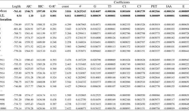
For the global-scale analysis, we calibrated the nonlinear mixed-effects model parameters ( and
’s) using training sets of 500 plots randomly selected (with replacement) from the GFB global
dataset according to the bootstrap aggregating (bagging) algorithm. We calibrated a total of
10,000 models based on the bagging samples, using our own bootstrapping program and the
nonlinear package nlme (62) of R, to calculate the means and standard errors of final model
estimates (Table 2). This approach overcame computational limits by partitioning the GFB
sample into smaller subsamples to enable the nonlinear estimation. The size of training sets was
selected based on the convergence and effect size of the geospatial random forest models. In
pilot simulations with increasing sizes of training sets (Fig.8), the value of elasticity of
substitution (31) fluctuated at the start until the convergence point at 500 plots. Generalized R2
value declined as the size of training sets increased from 0 to 350 plots, and stabilized at around
0.35 as training set size increased further. Accordingly, we selected 500 as the size of the
training sets for the final geospatial random forest analysis. Based on the estimated parameters of
the global model (Table 2), we analyzed the effect of relative species richness on global forest
productivity with a sensitivity analysis by keeping all the other variables constant at their sample
means for each ecoregion.
22 <Table 2>
Mapping BPR across global forest ecosystems
For mapping purposes, we first estimated the current extent of global forests in several steps. We
aggregated the 'treecover2000' and 'loss' data (66) from 30 m pixels to 30 arc-second pixels (~1
km) by calculating the respective means. The result was ~1 km pixels showing the percentage
forest cover for the year 2000 and the percentage of this forest cover lost between 2000 and
2013, respectively. The aggregated forest cover loss was multiplied by the aggregated forest
cover to produce a single raster value for each ~1 km pixel representing a percentage forest lost
between 2000 and 2013. This multiplication was necessary since the initial loss values were
relative to initial forest cover. Similarly, we estimated the percentage forest cover gain by
aggregating the forest 'gain' data (66) from 30 m to 30 arc-seconds while taking a mean. Then,
this gain layer was multiplied by 1 minus the aggregated forest cover from the first step to
produce a single value for each ~1 km pixel that signifies percentage forest gain from 2000–
2013. This multiplication ensured that the gain could only occur in areas that were not already
forested. Finally, the percentage forest cover for 2013 was computed by taking the aggregated
data from the first step (year 2000) and subtracting the computed loss and adding the computed
gain.
We mapped productivity P and elasticity of substitution (31) across the estimated current
extent of global forests, here defined as areas with 50 percent or more forest cover. Because GFB
ground plots represent approximately 40 percent of the forested areas, we used universal kriging
(cf. 61) to estimate P and for the areas with no GFB sample coverage. The universal kriging
23 parameters (i.e. nugget, range, and sill) specified in Fig.7. We obtained the best linear unbiased
estimators of P and and their standard error across the current global forest extent with the
gstat package of R (67). By combining estimated from geospatial random forest and universal
kriging, we produced the spatially continuous maps of the elasticity of substitution (Fig.3B) and
forest productivity (Fig.S1) at a global scale. The effect sizes of the best linear unbiased
estimator of (in terms of standard error and generalized R2) are shown in Fig.5. We further
estimated percentage and absolute decline in worldwide forest productivity under two scenarios
of loss in tree species richness— low (10% loss) and high (99% loss). These levels represent the
productivity decline (in both percentage and absolute terms) if local species richness across the
global forest extent would decrease to 90 and 1 percent of the current values, respectively. The
percentage decline was calculated based on the general BPR model (Eq.1) and estimated
worldwide spatially explicit values of the elasticity of substitution (Fig.3B). The absolute decline
was the product of the worldwide estimates of primary forest productivity (Fig.S1) and the
standardized percentage decline at the two levels of biodiversity loss (Fig.4A).
Economic Analysis
Estimates of the economic value-added from forests employ a range of methods. One prominent
recent global valuation of ecosystem services (68) valued global forest production (in terms of
‘raw materials’ provided by forests(TableS1 in 68)) in 2011 at US$ 649 billion (6.49×10¹¹, in
constant 2007 dollars). Using an alternative method, the UN FAO (25) estimates gross
value-added in the formal forestry sector at US$606 billion (6.06×10¹¹, in constant 2011 dollars). We
used these two reasonably comparable values as bounds on our coarse estimate of the global
economic value of forest productivity, converted to constant 2015 US$ based on the US
24 decrease of tree species richness distributed evenly across the world (from 100% to 90%) would
cause a 2.1–3.1 percent decline in productivity which would equate to US$13–23 billion per year
(constant 2015 US$). For the assessment of the value of biodiversity in maintaining forest
productivity, a hypothetical 99 percent drop in species richness would lead to 62–78% reduction
in forest productivity, equivalent to 396–579 billion US$ per year (3.96–5.79×10¹¹, constant
2015 US$). Therefore, we estimated that the economic value of biodiversity in maintaining
forest productivity worldwide would be 396–579 billion US$ per year.
Even though these estimates of the economic value-added from forest BPR employed two
starkly different methods, they were still reasonably close. We held the total number of trees,
global forest area and stocking, and other factors constant to estimate the value of productivity
loss solely due to a decline in tree species richness. As such, these estimates did not include the
value of land converted from forest and losses due to associated fauna and flora decline and
forest habitat reduction. This estimate only reflects the value of biodiversity in maintaining forest
wood productivity, and does not account for other values of biodiversity. The total global value
25
REFERENCES AND NOTES
1. S. Naeem, J. E. Duffy, E. Zavaleta, The Functions of Biological Diversity in an Age of Extinction. Science 336,1401-1406 (2012).
2. Millennium Ecosystem Assessment, “Ecosystems and Human Well-being: Biodiversity
Synthesis ” (World Resources Institute, Washington, DC, 2005)
3. J. Liang, M. Zhou, P. C. Tobin, A. D. McGuire, P. B. Reich, Biodiversity influences plant productivity through niche–efficiency. PNAS 112,5738-5743 (2015).
4. M. Scherer-Lorenzen, in Forests and Global Change, D. Burslem, D. Coomes, W. Simonson, Eds. (Cambridge University Press, Cambridge, 2014), pp. 195-238. 5. B. J. Cardinale et al., Biodiversity loss and its impact on humanity. Nature 486,59-67
(2012).
6. Y. Zhang, H. Y. H. Chen, P. B. Reich, Forest productivity increases with evenness, species richness and trait variation: a global meta-analysis. J. Ecol. 100,742-749 (2012). 7. A. Paquette, C. Messier, The effect of biodiversity on tree productivity: from temperate
to boreal forests. Global Ecol. Biogeogr. 20,170-180 (2011).
8. P. Ruiz Benito et al., Diversity increases carbon storage and tree productivity in Spanish forests. Global Ecol. Biogeogr. 23,311-322 (2014).
9. F. van der Plas et al., Biotic homogenization can decrease landscape-scale forest multifunctionality. PNAS 113,3557-3562 (2016).
10. F. Isbell, D. Tilman, S. Polasky, M. Loreau, The biodiversity-dependent ecosystem service debt. Ecol. Lett. 18,119-134 (2015).
11. S. Díaz et al., The IPBES Conceptual Framework — connecting nature and people. Current Opinion in Environmental Sustainability 14,1-16 (2015).
12. United Nations. (Nagoya, Japan, 2010), vol. COP 10 Decision X/2.
13. W. M. Adams et al., Biodiversity Conservation and the Eradication of Poverty. Science
306,1146-1149 (2004).
14. J. B. Grace et al., Integrative modelling reveals mechanisms linking productivity and plant species richness. Nature 529,390–393 (2016).
15. D. I. Forrester, H. Pretzsch, Tamm Review: On the strength of evidence when comparing ecosystem functions of mixtures with monocultures. For. Ecol. Manage. 356,41-53 (2015).
16. C. M. Tobner et al., Functional identity is the main driver of diversity effects in young tree communities. Ecol. Lett. 19,638-647 (2016).
17. K. Verheyen et al., Contributions of a global network of tree diversity experiments to sustainable forest plantations. Ambio 45,29-41 (2016).
18. FAO, “Global Forest Resources Assessment 2015 - How are the world’s forests
changing? ” (Food and Agriculture Organization of the United Nations, Rome, Italy,
2015)
19. H. Ter Steege et al., Estimating the global conservation status of more than 15,000 Amazonian tree species. Science advances 1,e1500936 (2015).
20. R. Fleming, N. Brown, J. Jenik, P. Kahumbu, J. Plesnik, in UNEP Year Book 2011 United Nations Environment Program, Ed. (UNEP, Nairobi, Kenya, 2011), pp. 46-59. 21. IUCN, IUCN Red List Categories and Criteria: Version 3.1. Version 2011.1. (Gland,
26 22. H. Pretzsch, G. Schütze, Transgressive overyielding in mixed compared with pure stands
of Norway spruce and European beech in Central Europe: evidence on stand level and explanation on individual tree level. Eur. J. For. Res. 128,183-204 (2009).
23. A. Bravo-Oviedo et al., European Mixed Forests: definition and research perspectives. Forest Systems 23,518-533 (2014).
24. K. B. Hulvey et al., Benefits of tree mixes in carbon plantings. Nature Climate Change
3,869-874 (2013).
25. FAO, “Contribution of the forestry sector to national economies, 1990-2011” (Food and Agriculture Organization of the United Nations Rome, 2014).Value-added has been adjusted for inflation and is expressed in USD at 2011 prices and exchange rates.
26. B. J. Cardinale et al., The functional role of producer diversity in ecosystems. Am. J. Bot.
98,572-592 (2011).
27. P. B. Reich et al., Impacts of biodiversity loss escalate through time as redundancy fades. Science 336,589-592 (2012).
28. M. Loreau, A. Hector, Partitioning selection and complementarity in biodiversity experiments. Nature 412,72-76 (2001).
29. D. Tilman, C. L. Lehman, K. T. Thomson, Plant diversity and ecosystem productivity: Theoretical considerations. PNAS 94,1857-1861 (1997).
30. H. Y. H. Chen, K. Klinka, Aboveground productivity of western hemlock and western redcedar mixed-species stands in southern coastal British Columbia. For. Ecol. Manage.
184,55-64 (2003).
31. The elasticity of substitution ( ), which represents the degree to which species can substitute for each other in contributing to stand productivity, reflects the strength of the effect of biodiversity on ecosystem productivity, after accounting for climatic, soil, and other environmental and local covariates.
32. H. Pretzsch et al., Growth and yield of mixed versus pure stands of Scots pine (Pinus sylvestris L.) and European beech (Fagus sylvatica L.) analysed along a productivity gradient through Europe. Eur. J. For. Res. 134,927-947 (2015).
33. E. D. Schulze et al., Opinion Paper: Forest management and biodiversity. Web Ecology
14,3 (2014).
34. R. Waring et al., Why is the productivity of Douglas-fir higher in New Zealand than in its native range in the Pacific Northwest, USA? For. Ecol. Manage. 255,4040-4046 (2008). 35. J. Liang, J. V. Watson, M. Zhou, X. Lei, Effects of productivity on biodiversity in forest
ecosystems across the United States and China. Conserv. Biol. 30,308-317 (2016). 36. L. H. Fraser et al., Worldwide evidence of a unimodal relationship between productivity
and plant species richness. Science 349,302-305 (2015).
37. M. Loreau, Biodiversity and ecosystem functioning: a mechanistic model. PNAS
95,5632-5636 (1998).
38. F. Isbell et al., Nutrient enrichment, biodiversity loss, and consequent declines in ecosystem productivity. PNAS 110,11911-11916 (2013).
39. C. Le Quéré et al., Global carbon budget 2015. Earth System Science Data 7,349-396 (2015).
40. A. Hector, R. Bagchi, Biodiversity and ecosystem multifunctionality. Nature 448,188-190 (2007).
27 42. D. P. McCarthy et al., Financial Costs of Meeting Global Biodiversity Conservation
Targets: Current Spending and Unmet Needs. Science 338,946-949 (2012).
43. C. B. Barrett, A. J. Travis, P. Dasgupta, On biodiversity conservation and poverty traps. PNAS 108,13907-13912 (2011).
44. B. Fisher, T. Christopher, Poverty and biodiversity: Measuring the overlap of human poverty and the biodiversity hotspots. Ecol. Econ. 62,93-101 (2007).
45. N. Myers, R. A. Mittermeier, C. G. Mittermeier, G. A. B. da Fonseca, J. Kent, Biodiversity hotspots for conservation priorities. Nature 403,853-858 (2000). 46. S. Gourlet-Fleury, J.-M. Guehl, O. Laroussinie, Ecology and management of a
neotropical rainforest: lessons drawn from Paracou, a long-term experimental research site in French Guiana. (Elsevier Paris, France, 2004), pp. 326.
47. J. C. Tipper, Rarefaction and rarefiction—the use and abuse of a method in paleoecology. Paleobiology 5,423-434 (1979).
48. M. L. Rosenzweig, Species Diversity in Space and Time. (Cambridge University Press, Cambridge, 1995), pp. 436.
49. L. Breiman, Random forests. Machine learning 45,5-32 (2001).
50. S. Chamberlain, E. Szocs, Taxize - taxonomic search and retrieval in R. F1000Research
2,191 (2013).
51. B. Husch, T. W. Beers, J. A. Kershaw Jr, Forest mensuration. (John Wiley & Sons, Hoboken, New Jersey ed. 4th, 2003), pp. 447.
52. M. G. R. Cannell, Woody biomass of forest stands. For. Ecol. Manage. 8,299-312 (1984).
53. M. Simard, N. Pinto, J. B. Fisher, A. Baccini, Mapping forest canopy height globally with spaceborne lidar. Journal of Geophysical Research: Biogeosciences 116 (2011). 54. N. L. Stephenson, P. J. van Mantgem, Forest turnover rates follow global and regional
patterns of productivity. Ecol. Lett. 8,524-531 (2005).
55. D. A. Clark et al., Measuring net primary production in forests: concepts and field methods. Ecol. Appl. 11,356-370 (2001).
56. ESRI, “Release 10.3 of Desktop, ESRI ArcGIS” (Environmental Systems Research Institute, Redlands, CA, 2014)
57. R Core Team, “R: A language and environment for statistical computing” (R Foundation for Statistical Computing, Vienna, Austria, 2013)
58. A. Di Gregorio, L. J. Jansen, “Land Cover Classification System (LCCS): classification
concepts and user manual” (FAO, Department of Natural Resources and Environment, Rome, Italy, 2000)
59. P. Legendre, Spatial autocorrelation: trouble or new paradigm? Ecology 74,1659-1673 (1993).
60. J. Liang, Mapping large-scale forest dynamics: a geospatial approach. Landscape Ecol.
27,1091-1108 (2012).
61. N. A. C. Cressie, Statistics for spatial data. (J. Wiley, New York, ed. Rev., 1993), pp. 900.
62. J. Pinheiro, D. Bates, S. DebRoy, D. Sarkar, R Development Core Team, nlme: Linear and Nonlinear Mixed Effects Models. (2011), vol. R package version 3.1-101.
28 64. A. Liaw, M. Wiener, Classification and regression by randomForest. R News 2,18-22
(2002).
65. L. Magee, R2 measures based on Wald and likelihood ratio joint significance tests. The American Statistician 44,250-253 (1990).
66. M. C. Hansen et al., High-resolution global maps of 21st-century forest cover change. Science 342,850-853 (2013).
67. E. J. Pebesma, Multivariable geostatistics in S: the gstat package. Computers & Geosciences 30,683-691 (2004).
68. R. Costanza et al., Changes in the global value of ecosystem services. Global Environ. Change 26,152-158 (2014).
69. BLS, in BLS Handbook of Methods. (US Department of Labor, Washington, DC, 2015). We used the online CPI calculator at: http://data.bls.gov/cgi-bin/cpicalc.pl.
70. T. Crowther et al., Mapping tree density at a global scale. Nature 525,201-205 (2015). 71. The tree drawings in the diagram were based on actual species from the GFB plots. The
scientific names of these species are (clockwise from the top): Abies nebrodensis, Handroanthus albus, Araucaria angustifolia, Magnolia sinica, Cupressus sempervirens, Salix babylonica, Liriodendron tulipifera, Adansonia grandidieri, Torreya taxifolia, and Quercus mongolica. Five of these ten species (A. nebrodensis, A. angustifolia, M. sinica, A. grandidieri, and T. taxifolia) are listed as endagered or critically endangered species in the IUCN Red List. Handdrawings were made by RK Watson.
72. Elevation consists mostly of ground-measured data and the missing values were replaced with the highest-resolution topographic data generated from NASA's Shuttle Radar Topography Mission-SRTM.
73. R. J. Hijmans, S. E. Cameron, J. L. Parra, P. G. Jones, A. Jarvis, Very high resolution interpolated climate surfaces for global land areas. International Journal of Climatology
25,1965-1978 (2005).
74. A. Trabucco, R. J. Zomer, in CGIAR Consortium for Spatial Information. (2009). 75. N. Batjes, “World soil property estimates for broad-scale modelling (WISE30sec)”
(ISRIC-World Soil Information, Wageningen, 2015)
29
ACKNOWLEDGMENTS
We are grateful to all the people and agencies that helped in collection, compilation, and coordination of the field data, including but not limited to T. Malone, J. Crowe, M. Sutton, J. Lovett, P. Munishi, M. Rautiainen, staff members from the Seoul National University Forest, and all persons who made the two Spanish Forest Inventories possible especially the main
coordinators, R. Villaescusa (IFN2) and J.A. Villanueva (IFN3). This work was supported in part by West Virginia University under the USDA McIntire-Stennis Funds WVA00104 and
WVA00105; U.S. National Science Foundation (NSF) Long-Term Ecological Research Program at Cedar Creek (DEB-1234162); the University of Minnesota Department of Forest Resources and Institute on the Environment; the Architecture and Environment Department of Italcementi Group, Bergamo (Italy); a Marie Skłodowska Curie fellowship; Polish National Science Center Grant 2011/02/A/NZ9/00108, the French ANR (CEBA: ANR-10-LABX-0025) and the General Directory of State Forest National Holding DB; General Directorate of State Forests, Warsaw, Poland (Research Projects No. 1/07 and OR/2717/3/11); the 12th Five-Year Science and
Technology Support Project (Grant No. 2012BAD22B02) of China; the U.S. Geological Survey and the Bonanza Creek Long Term Ecological Research Program funded by the National Science Foundation and the U.S. Forest Service (any use of trade, firm, or product names is for descriptive purposes only and does not imply endorsement by the U.S. Government); National Research Foundation of Korea (NRF-2015R1C1A1A02037721), Korea Forest Service
(S111215L020110, S211315L020120 and S111415L080120) and Promising-Pioneering
Researcher Program through Seoul National University (SNU) in 2015; Core funding for Crown
Research Institutes from the New Zealand Ministry of Business, Innovation and Employment’s
Science and Innovation Group; the DFG Priority Program 1374 Biodiversity Exploratories; Chilean research grants FONDECYT No. 1151495 and 11110270; Natural Sciences and Engineering Research Council of Canada (RGPIN-2014-04181); Brazilian Research grants CNPq 312075/2013 and FAPESC 2013/TR441 supporting Santa Catarina State Forest Inventory (IFFSC); General Directorate of State Forests, Warsaw, Poland; Bavarian State Ministry for Nutrition, Agriculture, and Forestry project W07; Bavarian State Forest Enterprise (Bayerische Staatsforsten AöR); German Science Foundation for project PR 292/12-1; European Union for funding the COST Action FP1206 EuMIXFOR; FEDER/COMPETE/POCI under Project POCI-01-0145-FEDER-006958 and FCT - Portuguese Foundation for Science and Technology under the project UID/AGR/04033/2013; Swiss National Science Foundation Grant 310030B_147092; and the European Union's Horizon 2020 research and innovation programme within the
30 The following authors have additional affiliations: Fernando Valladares is an Associate Professor
to the Universidad Rey Juan Carlos, Mostoles, Madrid, Spain; Tomasz Zawiła-Nied wiecki is also employed by the Polish State Forests; Jacek Oleksyn is affiliated to the Institute of
Dendrology, Polish Academy of Sciences, Poland, and University of Minnesota, Department of Forest Resources, USA. Thomas Crowther was at Yale School of Forestry, USA, when this work was initiated, and is now at the Netherlands Institute of Ecology.
We thank the following agencies and organization for providing the data: the United States Department of Agriculture (USDA) Forest Service; School of Natural Resources and
Agricultural Sciences, University of Alaska Fairbanks; the Ministère des Forêts, de la Faune et des Parcs du Québec (Canada); the Alberta Department of Agriculture and Forestry, the
Saskatchewan Ministry of the Environment, and Manitoba Conservation and Water Stewardship (Canada); the National Vegetation Survey Databank (New Zealand); Italian and Friuli Venezia Giulia Forest Services (Italy); Bavarian State Forest Enterprise (Bayerische Staatsforsten AöR) and the Thünen Institute of Forest Ecosystems (Germany); Queensland Herbarium (Australia); Forestry Commission of New South Wales (Australia); Instituto de Conservação da Natureza e das Florestas (Portugal). M'Baïki data were made possible and provided by the ARF Project (Appui la Recherche Forestière) and its partners: AFD (Agence Française de Développement), CIRAD (Centre de Coopération Internationale en Recherche Agronomique pour le
Développement), ICRA (Institut Centrafricain de Recherche Agronomique), MEDDEFCP (Ministère de l'Environnement, du Développement Durable des Eaux, Forêts, Chasse et Pêche),
SCAC/MAE (Service de Coopération et d’Actions Culturelles, Ministère des Affaires
Etrangères), SCAD (Société Centrafricaine de Déroulage), and the University of Bangui. All TEAM data were provided by the Tropical Ecology Assessment and Monitoring (TEAM) Network, a collaboration between Conservation International, the Smithsonian Institute and the Wildlife Conservation Society, and partially funded by these institutions, the Gordon and Betty Moore Foundation, the Valuing the Arc Project (Leverhulme Trust), and other donors; The Exploratory plots of FunDivEUROPE received funding from the European Union Seventh Framework Programme (FP7/2007-2013) under grant agreement no. 265171. The Chinese Comparative Study Plots (CSPs) were established in the framework of BEF-China, funded by the German Research Foundation (DFG FOR891); Data collection in Middle Eastern countries was supported by the Spanish Agency for International Development Cooperation (Agencia Española de Cooperación Internacional para el Desarrollo, AECID) and Fundación Biodiversidad, in cooperation with the governments of Syria and Lebanon. We are grateful to the Polish State
Forest Holding for the data collected in the project “Establishment of a forest information system covering the area of the Sudetes and the West Beskids with respect to the forest condition
monitoring and assessment” financed by the General Directory of State Forest National Holding.
31 The data used in this manuscript are summarized in the supplementary materials (Data Table S1-S2). All data needed to replicate these results are available at http://jiliang.forestry.wvu.edu/. New Zealand data are available from Susan Wiser under a material agreement with the National Vegetation Survey Databank managed by Landcare Research, New Zealand. Access to Poland data needs additional permission from Polish State Forest National Holding, as provided to
Tomasz Zawiła-Nied wiecki.
SUPPLEMENTARY MATERIALS
Figs. S1 to S3
Data Tables S1 to S2
32
Fig.1. Global forest biodiversity (GFB) ground-sourced data were collected from in situ
33
34
Fig.3. The estimated global effect of biodiversity on forest productivity was positive and concave-down (A) and revealed considerable geospatial variation across forest ecosystems worldwide(B). (A) Global effect of biodiversity on forest productivity (red line with pink bands representing 95 percent confidence interval) corresponds to a global average elasticity of substitution ( ) value of 0.26, with climatic, soil, and other plot covariates being accounted for and kept constant at sample mean. Relative species richness (Š) is in the horizontal axis, and productivity (P, m3ha-1yr-1) in the vertical axis
35
Fig.4. Estimated percentage (A) and absolute (B) decline in forest productivity under 10 and 99 percent decline in current tree species richness (values in parentheses correspond to 99 percent), everything else remained the same. (A) Percent decline in productivity was calculated based on the general BPR model (Eq.1) and estimated worldwide spatially explicit values of the elasticity of
substitution (Fig.3B). (B) Absolute decline in productivity, was derived from the estimated elasticity of substitution (Fig.3B) and estimates of global forest productivity (Fig.S1). The first 10 percent reduction in tree species richness would lead to 0.001–0.597 m3ha-1yr-1 decline in periodic annual increment, which
36
Fig.5. Standard error (A) and generalized R2 (B) of the spatially explicit estimates of elasticity of
substitution ( ) across the current global forest extent. Standard error increased as a location was
37
Fig.6. Correlation matrix (A) and importance values (B) of potential variables for the geospatial random forest analysis. There were a total of 15 candidate variables from three categories, namely plot attributes, climatic variables, and soil factors (see Table 1 for a detailed description). Correlation
38
Fig.7. Semivariance (gray circles) and estimated spherical variogram models (blue curves) obtained from geospatial random forest. There was a general trend that semivariance increased with distance, i.e.
spatial dependence of weakened as the distance between any two GFB plots increased. The final
39