Rochester Institute of Technology
RIT Scholar Works
Theses Thesis/Dissertation Collections
6-2017
Pipelined Implementation of a Fixed-Point Square
Root Core Using Non-Restoring and Restoring
Algorithm
Vyoma Sharma
Follow this and additional works at:http://scholarworks.rit.edu/theses
This Master's Project is brought to you for free and open access by the Thesis/Dissertation Collections at RIT Scholar Works. It has been accepted for inclusion in Theses by an authorized administrator of RIT Scholar Works. For more information, please [email protected].
Recommended Citation
PIPELINED IMPLEMENTATION OF AFIXED-POINTSQUAREROOTCOREUSING
NON-RESTORING AND RESTORINGALGORITHM
by
Vyoma Sharma
GRADUATEPAPER
Submitted in partial fulfillment of the requirements for the degree of
MASTER OFSCIENCE in Electrical Engineering
Approved by:
Mr. Mark A. Indovina, Lecturer
Graduate Research Advisor, Department of Electrical and Microelectronic Engineering
Dr. Sohail A. Dianat, Professor
Department Head, Department of Electrical and Microelectronic Engineering
DEPARTMENT OFELECTRICAL AND MICROELECTRONICENGINEERING KATE GLEASONCOLLEGE OFENGINEERING
ROCHESTER INSTITUTE OF TECHNOLOGY ROCHESTER, NEWYORK
I dedicate this work to my family and friends for their love, support and inspiration during my
Declaration
I hereby declare that except where specific reference is made to the work of others, that all
content of this Graduate Paper are original and have not been submitted in whole or in part for
consideration for any other degree or qualification in this, or any other University. This Graduate
Project is the result of my own work and includes nothing which is the outcome of work done in
collaboration, except where specifically indicated in the text.
Vyoma Sharma
Acknowledgements
I want to thank my advisor Mark A. Indovina for his support, guidance, feedback and
Abstract
Arithmetic Square Root is one of the most complex but nevertheless widely used operations in
modern computing. A primary reason for the complexity is the irrational nature of the square
root for non-perfect numbers and the iterative behavior required for square root computation. A
typical RISC implementation of Square Root Computation can take anywhere from 200 - 300
cycles. If significant usage is encountered, this could result in an impact in run-time cost which
would justify a direct hardware implementation that achieves the same result in as little as 20
clock cycles. Additionally, the implementation is pipelined to achieve even greater throughput
compared to an instruction based implementation. The paper thus presents an efficient, pipelined
implementation of a square root calculation core which implements a non-restoring algorithm of
determining the square-root. The iteration count of the algorithm depends on the maximum size
of the input and the desired resolution. A specific case of a 16-bit integer square root calculator
with output resolution 0.001 is considered which requires a total of 18 iterations of the algorithm.
In the implementation, each iteration is pipelined as a stage thereby resulting in an 18-stage
pipelined square root computation core. The proposed algorithm utilizes standard arithmetic
operations like addition, subtraction, shift and basic control statements to determine the output
of each stage. The core is verified using SystemVerilog test-bench. The test-bench generates
unconstrained random inputs stimulus and determines the expected value from the core device
under test (DUT) by evaluating a Simulink generated model for the same stimulus. Functional
v
Contents
Contents vi
List of Figures ix
1 Introduction 1
1.1 Concept of Operation . . . 2
1.1.1 Stage I . . . 3
1.1.2 Stage II . . . 3
1.1.3 Stage III . . . 4
1.2 Research Goals . . . 5
1.3 Organization . . . 5
2 Bibliographical Research 6 3 System Architecture 13 4 Detail Design 15 4.1 Non-Restoring Algorithm . . . 15
4.1.1 Implementation . . . 16
Contents vii
4.2.1 Implementation . . . 18
5 Verification Methodology and Results 20 5.1 Verification Methodology . . . 20
5.2 Test Bench Design and its Components . . . 21
5.2.1 Layered Test Bench Architecture . . . 21
5.2.1.1 Interface . . . 23
5.2.1.2 Stimulus . . . 24
5.2.1.3 Scoreboard . . . 24
5.2.1.4 Driver . . . 25
5.2.1.5 Model . . . 25
5.2.1.6 Monitor / Checker . . . 25
5.2.1.7 Environment . . . 26
6 Results 27 6.1 Non-Restoring . . . 28
6.2 Restoring . . . 29
7 Conclusion 32 References 34 I Source Code 38 I.1 Non-restoring Algorithm . . . 38
I.1.1 Non-Restoring Algorithm Operation . . . 38
I.1.2 Non-Restoring Algorithm with Pipeline architecture . . . 39
Contents viii
I.1.4 Driver . . . 57
I.1.5 Model . . . 59
I.1.6 Monitor . . . 64
I.1.7 Test Bench . . . 66
I.2 Restoring Algorithm . . . 67
I.2.1 Restoring Algorithm Operation . . . 67
I.2.2 Non-Restoring Algorithm with Pipeline architecture . . . 68
I.2.3 Environment . . . 85
I.2.4 Driver . . . 86
I.2.5 Model . . . 89
I.2.6 Monitor . . . 93
List of Figures
4.1 Non-Restoring Square Root Calculation for a single stage . . . 16
4.2 Restoring Operation . . . 18
4.3 Restoring Algorithm for a single stage iteration . . . 18
5.1 Lower Layers of the Verification Test Bench . . . 22
5.2 Test Bench Schematic for Verification . . . 23
5.3 Interface Block Diagram . . . 23
6.1 Coverage Report for Restoring/Non-Restoring Algorithm . . . 27
6.2 Pipeline Data flow for Non-Restoring Algorithm . . . 28
6.3 Data transition from Input to Output . . . 29
6.4 Pipeline Data flow for Restoring Algorithm . . . 30
Chapter 1
Introduction
Square root is one of the fundamental arithmetic operations used by various signal and image
pro-cessing algorithms apart from addition, subtraction, multiplication and division. Typical square
root algorithms compute bits successively starting with the most significant bit and predicting
the lower significant bit. The correctness of the predicted value is determined by comparing the
square of the predicted number and the remainder determined for the particular stage. In this
research paper, two similar algorithms to compute the square root of an integer number have
been taken into consideration and extended to determine the fixed point fractional square root
of the number. The paper characterizes the implementation of the two square root algorithm
namely restoring algorithm and non-restoring algorithm. Non-restoring algorithm is the simpler
and more efficient technique as it uses for square root implementation as it uses
adders/subtrac-tors and shift operations to determine the square root of the number. The characteristic difference
between the algorithms, is their approach towards the selection of the square root digit and the
partial remainder determination. The implemented system would utilize fixed-point
nomencla-ture to represent the numbers as they require fewer pre-processing compared to floating-point
1.1 Concept of Operation 2
consuming larger number of cycles for computation compared to their equivalent fixed-point
arithmetic cores. However fixed-point arithmetic truncates bits lower than the significant range
of the number. This becomes especially significant in case of smaller numbers whose relative
value is drastically impacted by the truncated bits.
SystemVerilog is an extension of the traditional Verilog Hardware Description Language
(HDL) which supports object oriented programming. The implemented test bench is constructed
hierarchically with multiple modular components. A SystemVerilog test bench which performs
unconstrained random verification of the functional core is utilized to verify the operation of
the implemented system. The expected value of the system is determined by a model which in
real-time determines the expected output of the ideal system for the same input stimulus vectors.
The model was developed using Matlab and is exported using the standard Simulink HDL code
library.
1.1
Concept of Operation
Considering the square root computation of a 16-bit integer number I[15:0], the result would be
an 8-bit integer number B[7:0] and infinite fractional bits B[-1:−∞]. Thebirefers to the ithe bit
of the numberB. TheBnrefers to the sub-set of theB,B[n:−∞].
I=B2
1.1 Concept of Operation 3
1.1.1
Stage I
I= (b27.214+2.b7.27.B6.+B26)
I= (b27.214+4.b7.26.B6+B26)
I−qb27.214y= (2.b7.27.B6) +B26
The Left hand side term is the remainder of the operation of stage I,RO1=I−qb27.214yand
the coefficient of 2.27B6, is the partial quotient estimated at Stage 1,QO1=b7.
1.1.2
Stage II
RI2=RO1= I−qb27.214y= (4.b7.26.(b6.26+B5)).+ (b6.26+B5)2)
RI2= (4.b7.b6.212) + (4.b7.B5.26) +b26.212+2b6B5.26+B25
RI2=q((4.b7+b6).b6).212y+2.|b7b6|.26.B5+B25
RI2−q((4.QO1+b6).b6).212y=2.|b7b6|.26.B5+B25
The Left hand side term is the remainder of the operation of stage II, RO2 = RI2−
q
((4.QO1+b6).b6).212yand the coefficient of 2.26B5, is the partial quotient estimated at Stage
1.1 Concept of Operation 4
1.1.3
Stage III
RI3=RO2=RI2−q((4.b7+b6).b6).212y=2.|b7b6|.26.b5.25+B4+b5.25+B42
RI3=2.|b7b6|.b5.211+2.|b7b6|.26.B4+b25.210+26.b5.B4+B24
RI3=q4.|b7b6|.b5.210+b25.210
y
+ (2.|b7b6|+b5).26.B4+B24
RI3=q4.|b7b6|.b5.210+b25.210
y
+|b7b6b5|.26.B4+B24
RI3−q(4.QO2+b5).b5.210y=|b7b6b5|.2.25.B4+B24
The Left hand side term is the remainder of the operation of stage III, RO3 = RI3−
q
(4.QO2+b5).b5.210y and the coefficient of 2.25B4, is the partial quotient estimated at Stage
II,QO3=|b7b6b5|.
Thus, for each stage operation an additional bit of the quotient is determined, thereby,
im-proving the resolution of the calculated square root result. Hence, the number of stage iterations
required depends on the input size and is relate-able to the required output square root resolution.
Consolidating the stage operations and assuming RI1= Input Data we get,
ROn= (RIn>(QIn≪2+1)?(RIn−(QIn≪2+1):RIn
1.2 Research Goals 5
The quotient at the output of the last stage is the resultant square root of the configured
resolution.
1.2
Research Goals
The objective of this paper is to identify and implement a simple and efficient algorithm to
evaluate the square root operation on large data sets. Two algorithms have been chosen for
this implementation, one is a non-restoring algorithm and the other is restoring algorithm. The
paper compares the two algorithm in terms computational complexity, basic number of arithmetic
operations required, number of resources needed and hardware cost.
1.3
Organization
The structure of the research paper is as follows:
• CHAPTER 2 Bibliographical Research: The chapter summarizes the existing research and
algorithms on efficient computation methods for evaluating the square root of a number.
• CHAPTER 3 System Architecture: The chapter describes the requirements and design of
the square root computational system.
• CHAPTER 4 Implementation: The chapter describes pipeline design implementation of the
Non-Restoring and Restoring algorithms.
• CHAPTER 5 Verification Methodology and Results: The approach taken for verification of
the design is discussed in this chapter.
• CHAPTER 6 Results: The results of the restoring and non-restoring algorithms are
dis-cussed in this chapter.
Chapter 2
Bibliographical Research
The most important step in implementing a square root core is to identify a simple, efficient,
iterative method of evaluating the square root of a given number. There are different methods of
evaluating the square root like recursive approximation method and other methods. Substantial
research is required to identify the method which would allow the implemented system to be
power and area efficient while still providing the required boost throughput which would justify
an implementation. Some of the research and methods of determining the square root of a
fixed-point number are documented in the chapter.
Select research papers consulted for the work are briefly discussed in this chapter.
Wang et al. in [1] presents a new algorithm based on the conventional Non-restoring
al-gorithm is implemented using Verilog HDL. This alal-gorithm alal-gorithm can be used on general
purpose FPGA chips and can be used to calculate square root for a 2n bit integer. The algorithm
developed is compared with the general algorithms for square root calculation based on the
num-ber of clock cycles required for the desired output, numnum-ber of resources required to implement
the algorithm and the number of pipeline stages required to calculate the square root of 16-bit
im-7
plemented on a general-use FPGA since it does not need a special hardware structure. Another
advantage is that n number of clock cycles are needed for a 2n bit integer and the speed for
pro-cessing the 2n bit integer is more as compared to other algorithm i.e. pipeline stages needed to
compute the output are less.
Yamin et al. in [2] illustrates two new implementations of non-restoring algorithm which
unlike the traditional algorithm does not focus on each bit of the square root rather depends upon
the partial remainder. Algorithm reduces the need for additional resources, like multiplexors,
multipliers, or seed generators and improves the resolution of the result for the last bit position.
The iterations are simpler as either addition/subtraction is carried out based on the last iteration
resultant bit.
The two algorithms differ in the implementation approach, one of the algorithms is a
high-performance pipeline implementation and second other compromises on speed but is a low-cost
implementation that uses less hardware. The algorithms implemented by Rachmad are proved to
be time and area efficient than most of the existing algorithms. Paper clearly shows the contrast
between the two implementations based on the number of cycles required for 16, 32 and 64-bit
data and the number of gates required for 16, 32 and 64-bit data.
Rachmad et al. [3]in writes about a new approach to calculate square root of a given
in-teger value. The author discusses first about the past researches on the square root calculation
approach and explains the implementation of the algorithms which used the binary input
de-composition approach. The algorithms discussed under previous works are Restoring algorithm
and Non-restoring algorithm which compute square root on the same concept of binary input
decomposition.
The author discusses the digital hardware implementation of the proposed algorithm and the
advantages of the new algorithm over the past researched approaches. The hardware design uses
8
module. The architecture is iterative in nature. It is a simple architecture that greatly reduces the
need for additional resources in the design. Thus, the number of clock cycles needed to obtain an
output depends upon the n-bit input. Therefore, (n/2) + 1 clock cycles are needed by the design
to complete the square root calculation. The author summarizes the simulation and synthesis
results for 32-bit and 64-bit data, considers number of clock cycles, clock speed, logic elements,
logic registers and combinational functions needed for the design.
Richard et al. [4].in presents implementation of two high-speed square root calculation
tech-niques which utilizes minimum number of computations. The author concentrates more on the
square root approximation algorithms which can be efficiently implemented in fixed-point
arith-metic. The constraints set on the algorithms by the author are: the division operation is not being
considered for calculation, the number of iteration should be less and a lookup table could be
used if required.
The two iterative methods discussed in the paper to determine the square root of a single
integer value are Newton-Raphson Inverse (NRI) method and Non-Linear IIR Filter (NIIRF)
method. The Newton-Raphson method is not recommended for fixed-point format rather it is
most suitable for floating-point systems. In this method chances of error increases if bits are
used to represent internal results. Second algorithm, Non-Linear IIR Filter (NIIRF) is another
iterative technique for a fixed-point implementation. Thus, the algorithms are compared for
accuracy versus computational cost/workload and the author concludes it by choosing NRIIF for
fixed-point math implementations.
The other high-speed square root methods discussed are Binary-Shift Magnitude estimation
and equiripple error magnitude estimation for complex number magnitude estimation.
Anuja et al. presents in [5] an algorithm that calculates square root of an 8-bit fixed and
floating-point number in a Field programmable Gate Array (FPGA) using the previously
Non-9
Restoring algorithms and implementation of a new module Controlled subtract multiplex in the
modified non-restoring algorithm.
This new algorithm proposed eliminates the components without affecting the resolution,
remainder and precision of the output. The author shows that the proposed algorithm is resource
efficient than the existing non-restoring algorithms. The difference highlighted between the two
algorithms is that the proposed algorithm does only subtraction operation and appends 01. It also
introduces a new module, controlled subtract multiplex for algorithm to compute square root for
any number of input bits. The comparison is tabulated for implementation with and without
optimization (CSM). Concludes by proving that the non-restoring algorithm consumes less area
on the chip and using a pipeline architecture improves the speed of the system.
Yamin et al. describes in [6] two single precision floating point square root design
imple-mentations based on the existing non-restoring algorithm. The two algorithms are implemented
on a general-use FPGA. The first algorithm is iterative implemented that uses a subtractor/adder
component and the design implementation is low on cost. The second algorithm is implemented
in a pipeline fashion and on every clock cycle it accepts a square root instruction.
The paper briefly discusses other algorithms like New-Raphson algorithm and
Sweeney-Robertson-Tocher (SRT) algorithms for square root extraction. The author describes the
archi-tecture and the implementation methodology for Non-Restoring square root algorithm,
Parallel-array implementation and single precision floating point square root algorithm. The algorithms
are compared on the latency, errors encountered and cost of design implementation. The two
iterative square root algorithms require less area on chip and the pipelined system has better
performance.
Atul et al. proposes in [7] a new algorithm to calculate the square root of an N-bit unsigned
number. Two architecture design implementation have been discussed. First design has a pipeline
10
square root of a N-bit fixed point number. The results of the existing and new algorithms have
been compared and the author shows that the new square root algorithm is far more efficient,
requires less clock cycles and less hardware.
First algorithm proposed has a pipeline architecture which constitutes of a subtractor and
compartor module. The second algorithm proposed with asynchronous architecture proves to
use less number of resources and has increased maximum operating frequency. Paper briefly
discusses the existing non-restoring square root algorithm, new technique to design pipeline
architecture for the non-restoring algorithm and asynchronous design for square root calculation
of a 32-bit number using modified non-restoring algorithm. The total time needed for square root
calculation significantly decreases in cases of a pipeline architecture.
Puneet et al. in [8] writes about a square root algorithm based on vedic mathematics formula
called Dwandwa Yoga. The inputs to the algorithm are 24-bit floating point number and 16-bit
floating point output. The author describes the existing algorithms for square root calculation
and compares the existing algorithms with the new implementation. The new algorithm is
im-plemented on SPARTAN-3E FPGA, this algorithm greatly reduces the complexity of the design.
Simulation and synthesis results tabulated in the paper clearly proves that the new
implementa-tion consumes less area, power and is operable at high frequencies.
Sajid et al. in [9] presents a new algorithm for square root calculation which reduces the
hazards of pipelining. The new proposed algorithm is based on the non-restoring algorithm
and architecture is designed such that it can be modified to adapt as per the requirements of an
application.
Read before write (RBW) hazard is avoided by the improved architecture of the algorithm
by replacing an condition with a NOT gate. Synthesis produced a multiplexer when an
if-condition was encountered, a multiplexer is a costly piece of hardware. Thus, the author improves
11
bits, accuracy of the result and for perfect combination of time, area and power.
Majerski et al. in [10] describes two algorithms for square root computation of addition of
two numbers. The algorithm presented in the paper is designed for high-speed digital circuits.
The algorithms are based on the non-restoring technique. Algorithm implemented differs with
the previously researched algorithms in a way that the addition and subtraction by taking the carry
as the third bit and considering the third bit while performing addition of three summands. Two
summands then form a partial remainder. The most significant bits determine the conventional
notation bits.
Montuschi et al. in [11] performs a survey of the square rooting algorithm. The algorithms
are discussed in detail by taking into consideration their properties. Author gives his final
com-ments on the effective and ideal implementation. The algorithms discussed are of two types:
iterative technique and approximation by real functions. The algorithms reviewed under iterative
technique is based on three classes: direct method, Newton-Raphson formula based algorithms
and normalization method. Pure hardware implementations can be done using direct methods
and the other iterative method applications can be done in hardware and software. Some of
the commonly used iterative method are Newton-Raphson algorithm, CODIC, DeLugish’s and
Chen’s algorithm. Among all these iterative algorithms, Newton -Raphson results are accurate.
Another approach for square root calculation is approximation by real functions. Taylor and
McLaurin series and Chebyshev polynomials are some of the real function approximation
tech-niques. The paper discusses in detail about the advantages and disadvantages and the application
of all the algorithms. The author focuses more on the algorithms that can be implemented on
hardware.
Bannur et al. in [12] discusses implementation of two non-restoring square root algorithms,
one using Barrel shifter implementation and second without the usage of Barrel shifter and
12
on chip, number of cycles needed for square root calculation and resources needed for
implemen-tation. The algorithms presented are simple and easy to implement and achieves better precision
compared to existing algorithms.
Using additional logic at the input of the Barrel shifter reduces the number of gates needed
by half. Three bits are modified in one iteration and the value depends upon the sign in the
previous iteration. Second algorithm implementation avoids the usage of Barrel shifter, instead
the same operation is achieved by adding registers of size 2n-bits and shifting it every cycle.
Second implementation proves to be better in terms of area needed on chip and time needed to
compute the result. Both implementations also discusses the floating-point implementation and
rounding of the last bits.
Chapter 3
System Architecture
The goals of the system requirement is to implement a core that calculates the square root of a
given integer operand. A 16-bit unsigned integer input is considered, whose square root has to be
calculated within a resolution of±1×10⁻³. The value of the output depends upon the number
of bits at the input, input resolution and the number of fractional bits generated at the output.
Since, the input is 16-bit unsigned integer, thus having unity resolution, the calculated square
root has 8 bits as the integer square root of the number. The rest of the bits would constitute the
fractional part of the solution. Square root calculator is implemented as a recursive operation,
where number of times the stage algorithm is performed determines the number of bits at the
output. The resolution of the output depends on the input size, resolution of the input and number
of stages. A generic formula for determining the number of stages is:
resolution≥2ceiling(K/2)−n
Where, K is the most significant bit position of the input, n is the number of stages.
Width of the solution depends upon the number of stages. The significance of the solution
14
Therefore for the give system requirements, the value of K is 15 (16 bit number
with unity resolution), thus the significant position of the MSB of the solution would be
f loor((log2(65535+1) +1)/2) =8. The required length of the fractional bits depends on the
required resolution. Each additional bit, after the integer increases the resolution by a factor of
1/2. Therefore the resolution of the output is given by 2−n, where n is the number of fractional
bits. Since the system specifies the resolution to be±0.001, the number of stages can be derived
as:
0.001≥2−n
This gives the possible values for n, which should be greater than 9 in order to achieve the
necessary resolution. In order to minimize hardware costs, while still attaining the requirements,
the minimum possible stage number of 10 is chosen to generate the fractional part.
Therefore the total number of stages, and consequently bits in the solution is 8 + 10 = 18
stages, with the MSB of the output having a significance of 28. The actual resolution of the
output is 2−10= 0.00098, which is less than the resolution requirement of the system.
Since the stage operations depend only on the previous stage output data the system can
be pipelined at the stage boundaries by registering the current output and allowing the stage to
process new inputs in the next clock cycle. As a result the 18 stage implementation can thus be
split into 18 stage pipeline resulting in higher throughput while reducing the operational speed
Chapter 4
Detail Design
The non-restoring and restoring algorithm of the iterative stage of the square root operation are
discussed below.
4.1
Non-Restoring Algorithm
Non-restoring algorithm is an iterative square root determination which generates one bit of a
result in each iteration using two most significant bits of the input data. The partial dividend
used for each iteration is determined by considering the remainder of the previous iteration and
appending the two most significant bit to the least significant position of the remainder. The
stage quotient is is computed as the previous iteration quotient shifted by one (to denote the
position significance) and appended with predicted new bit value (Qn=Qn−1≪1+1), the
subtrahend is determined as the previous iteration quotient shifted by two and appended with the
new predicted quotient bit value. If the value the new dividend is greater the subtrahend then,
then predicted value is accepted and the difference is forwarded as the remainder for the next
4.1 Non-Restoring Algorithm 16
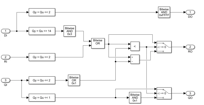
Figure 4.1: Non-Restoring Square Root Calculation for a single stage
forwarded as the remainder of the current iteration.
4.1.1
Implementation
A single iteration of the algorithm generates one bit of the square root output. The
implemen-tation is constructing by cascading multiple stages of the iteration with data storage elements
isolating the stage for pipelined implementation. The Data Input to the stage is provided by the
Data Output of the previous stage, which in turn is the shifted version of the original input data.
The Remainder In for the current stage is provided by the Remainder Out of the previous stage.
The Remainder In and the two most significant bits of the Data Input are used to construct the
minuend for the stage operation. The subtrahend is determined from the Quotient In, which is
provided by the Quotient Out of the previous stage and a assumed new bit value (1’b1). If the
subtrahend is greater than or equal to the minuend ( condition = 1 ), then the predicted quotient
is accepted and the remainder out is updated with the non-negative difference; else the predicted
quotient is discarded ( changed to 0 ) and the minuend is forwarded as the remainder out for the
4.2 Restoring Algorithm 17
The inputs for all stages is cascaded from the previous stage. The Quotient Input and
Re-mainder Input of the first stage is assumed to be 0 and the input integer data is fed to the Data
Input for the first stage.
input DI, QI, RI;
output DO, QO, RO;
wire rtemp, condition ;
assign rtemp = { RI , DI[15:14] };
assign condition = (rtemp >= {QI, 2’b01});
assign DO = {DI[13:0], 2’b00};
assign RO = condition ? rtemp - {QI,2’b01} : rtemp ;
assign QO = condition ? {QI,1’b1} : {QI,1’b0} ;
4.2
Restoring Algorithm
The restoring algorithm is an alternate method of computing the square root of a number, which
differs from the Non-Restoring algorithm, primarily in dealing with the decision making step
to determine the new quotient bit. The algorithm assumes a new quotient bit to be 1, and
proceeds to evaluate the subtraction operation by deducting the newly determined subtrahend
((Qn−1<<2) +2′b01)from the minuend to determine the Remainder Out. An incorrect guess
results in a negative remainder, which is identified by checking the sign bit (MSB) of the
remain-der. In the next iteration, if a negative remainder is detected, the system restores the previous
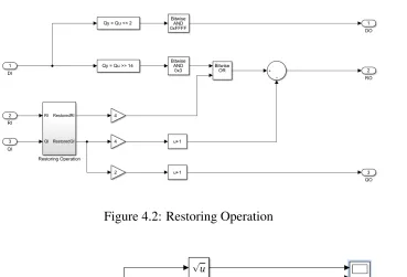
4.2 Restoring Algorithm 18
[image:29.612.137.474.319.403.2]Figure 4.2: Restoring Operation
Figure 4.3: Restoring Algorithm for a single stage iteration
4.2.1
Implementation
A single iteration of the algorithm generates one bit of the square root output. The
implemen-tation is constructed by cascading multiple stages of the iteration with data storage elements
isolating the stage for pipelined implementation. The Data Input to the stage is provided by the
Data Output of the previous stage, which in turn is the shifted version of the original input data.
The Remainder In for the current stage is provided by the Remainder Out of the previous stage.
The Remainder In and the two most significant bits of the Data Input are used to construct the
minuend for the stage operation. The subtrahend is determined from the Quotient In, which is
4.2 Restoring Algorithm 19
assumed data is provided as the stage output. The minuend, based on the new predicted quotient
bit 1 is subtracted from the subtrahend and the resultant remainder (+/−) is provided as the
Remainder Out of the current stage. At the start of the iteration, if the partial remainder input to
the block is negative the last assumed quotient bit is cleared and the subtraction performed in the
previous stage is reverted and the remainder is restored to the previous value.
The inputs for all stages is cascaded from the previous stage. The Quotient Input and
Re-mainder Input of the first stage is assumed to be 0 and the input integer data is fed to the Data
Input for the first stage.
input DI, QI, RI;
output DO, QO, RO;
wire condition, rRestd, qRestd ;
assign condition = RI >> (2*StageNum-2) ; // Extraction of the sign-bit
assign qRestd = condition ? {QI[StageNum:1], 1’b0} : QI ; // Fixes the incorrect guess of the
quotient
assign rRestd = condition ? RI + {qRestd,1’b1} : RI ; // Fixes the incorrect guess of the
remainder
//Rest of algorithm for unconditional subtract for qn = 1’b1
assign DO = { DI[13:0], 2’b00 } ; // Left shifting the DataIn by 2
assign RO = { rRestd , DI[15:14] } - { qRestd , 2’b01 } ; // Subtra
Chapter 5
Verification Methodology and Results
5.1
Verification Methodology
A test bench is implemented using SystemVerilog [21–26] to verify the operation of the
restor-ing and non-restorrestor-ing algorithm for square root computation. A stream of unconstrained 16-bit
random integers is used as a input to verify system operation. The test bench contains an
accu-rate model of the square root computation with delays to simulate pipeline operation. Therefore,
when the same input is fed into the device under test (DUT) and the model provides the expected
response which is compared with the DUT output to verify the accuracy of the calculation.
The steps to verify the system are generation of inputs, initial reset of DUT and reference
model, capture the output of DUT and model, verification of correctness of the output and the
errors or issues are reported for a solution. Since random vectors are used for verification
func-tional coverage of the input vectors is utilized as the control parameter to decide the duration the
5.2 Test Bench Design and its Components 21
5.2
Test Bench Design and its Components
The test bench should generate input vectors, provides the input to the DUT, determines the
expected output, monitors the output of the DUT, compare the expected and actual output of the
system, collect data and coverage statistics pertaining to the executed test cases, regulate test
duration and monitor the overall performance of the system. A modular test bench architecture
is adapted which consists of a network of objects, that perform the various operations required
to test the system. A modular or layered architecture is preferred to test complex systems as it
supports reuse of the developed components and the encapsulation of data and member functions;
allows different blocks to be easily modified for changes in the system like change in input size,
or data transmission protocols.
5.2.1
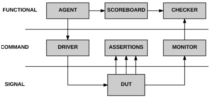
Layered Test Bench Architecture
A layered architecture is preferred as a common verification environment as it results in blocks
that are reusable and extendable to be taken advantage of during test automation. There are three
layers in a test bench known as Signal layer, Command layer and Scenario layer. The signal
layer being the lowest layer the architecture, it connects the test bench with the RTL design.
This layer comprises of DUT and has interface, modports and clocking modules. The command
layer gives transaction-level interface to the next layer and drives the pins through signal layer.
The command consists of a driver. The third layer is the functional layer, that consists of
driver-monitor components and has a self-checking construction. This layer determines of the test cases
fail or pass. This type of layered test bench is typically used for a constrained-random stimulus
5.2 Test Bench Design and its Components 22
Figure 5.1: Lower Layers of the Verification Test Bench
The components of the test bench are instantiated hierarchically and called in phases to
ini-tialize, execute and complete every test [27]. The test bench components are shown in the block
diagram in the figure below.
A verification methodology which has random test cases have been adapted to check the
square root operation of the DUT. The inputs to the DUT are unconstrained random vectors to
which the output is monitored and compared to the simulated the response of the system.The test
bench is methodically is split into components to allow versatility and flexibility of use in the
system.
5.2 Test Bench Design and its Components 23
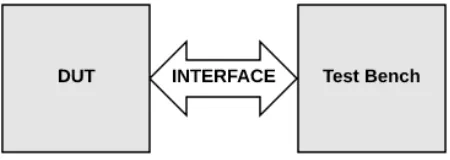
Figure 5.2: Test Bench Schematic for Verification
5.2.1.1 Interface
An interface encapsulates the required connections between a hardware block and the external
system. It can also serve as a connection between the DUT, a hardware block and the test bench,
which is a software component . It captures the communication between the blocks including
the connectivity, directional information, clocking blocks. It ensures there is no duplication of
connections, the port list for connections are compact and it easy to change to integrate to higher
levels.
Figure 5.3: Interface Block Diagram
An external clock is is provided to the interface, which forwards it to the test bench for
[image:34.612.194.419.502.582.2]5.2 Test Bench Design and its Components 24
for the interface class and is mapped to the outermost interface inside the different components
of the test bench..
5.2.1.2 Stimulus
The stimulus module consists of a randomizable 16-bit vector which is used for the generation of
inputs for the device under test and the model. In this test bench since the system should respond
uniformly for all possible inputs, unconstrained random number generator is used to generate the
inputs for verification.
/* *
* Author: Vyoma Sharma
* Rochester, NY, USA
* Description: Stimulus generates the random numbers.
* */
class stimulus;
rand bit [15:0] data;
endclass
In SystemVerilog, a class, containing a rand variable, is inherently defined with a randomize()
function which generates a new random number based on the previously defined seed value.
Therefore calling the randomize() function generates the new input which is then fed into the test
bench.
5.2.1.3 Scoreboard
The scoreboard is the generic whiteboard for the test bench, it can store data which can be
hori-zontally shared among the various components of the test bench, Typically the scoreboard may
5.2 Test Bench Design and its Components 25
statistics like number of tests and other test related information. The use of scoreboard is optional
when utilized with a well defined checker and functional coverage components.
5.2.1.4 Driver
The Driver operates as the conduit between the transaction layer and signal layer of the testbench.
The inputs generated are at high level of abstraction and thus, these inputs are converted to actual
design inputs. It accepts input data sets from the Stimulus, synchronizes and provides the input
dataset to the actual input ports of the DUT. It also operates the necessary write protocols and
signals required for the DUT to recognize the valid data provided by the driver.
5.2.1.5 Model
The model is high level embodiment of the requirements of the device under test. It is typically
implemented with a high level of abstraction, where the requirements can be easily met, but is
not suitable for synthesis and implementation. The validity of the device relies of the accuracy of
the model. In the current test bench, the model required to capture the intent of the algorithm is
generated from Simulink. The code is generated for the square root operation which has a 16-bit
unsigned integer input and a 18-bit (8,10) fixed point output. A cascaded delay block is used to
simulate the operation of the pipeline in the system.
5.2.1.6 Monitor / Checker
The monitor block monitors the output interface ports and receives and assembles the actual data
from the device under test. It checks for any communication protocol violation and determines
the value of the complete transactions [28]. Monitor also consists of coverage and assertions
features to ensure the system behavior is met and tested. The output of the monitor is transaction
5.2 Test Bench Design and its Components 26
The checker operates on the transaction data received from the monitor and the reference
data from the model. The checker compares the monitor output and the model output to ensure
functional correctness of the device operation. In this system, since the output of the device
under test is parallel 18-bit output data, the role of the monitor is greatly reduced and therefore
the monitor and checker are combined to a single test bench component [28].
5.2.1.7 Environment
The environment serves as the container in which the components of the test bench are
instan-tiated. The various components classes are instantiated and connected to each other thereby
constituting the complete test bench. The environment can also contain a program that
exe-cutes the various initializes and exeexe-cutes the various components used, while implementing the
Chapter 6
Results
The implementation of the restoring and non-restoring algorithm for square root computation
was successfully verified. Since the input was 16-bits the output bit with required in order to
achieve 0.001 resolution was confirmed to be 18-bits with 10-bits representing the fractional
portion of the calculated square root value. This gives the solution an effective resolution of 2−10
approximately 0.000977, which meets the system specification of at least 0.001 resolution. The
resolution of the result can be improved by adding additional computation stages to the system.
Functional coverage was used to ensure that the system has been tested for all possible input
values. The implemented functional coverage checks if all the bins corresponding to each
pos-sible input is set at least once before the test is terminated. This results in some of the inputs
being tested more often than others but all the inputs are tested at least once and system
opera-tion is verified for all the inputs. Below are the coverage report for non-restoring and restoring
algorithm.
6.1 Non-Restoring 28
Issues were faced while implementing the test bench for non-restoring algorithm and
restor-ing algorithm. In the test bench, a malfunction was detected in it’s operation which substantially
increased run-time and processing power required for the test bench evaluation. The root cause
of the problem was identified as incorrect interfacing between the hardware signals and the
soft-ware test bench. The looping statement introduced in the monitor to check at every edge of the
clock if the DUT output is identical to the model output was implemented without considering
synchronization with the clock. This resulted in the system evaluating an infinite loop between
clock edge events causing the system to stall indefinitely at the loop. This was resolved by
including an instruction to execute each iteration of the loop for each rising edge of the clock.
6.1
Non-Restoring
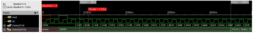
Cursor at TimeA and TimeB indicates that the clock period is 20 ns. The time taken to complete
the entire square root computation for a single input is 360 ns (TimeC - TimeA), thus the system
[image:39.612.84.526.461.519.2]evaluates the 18 bit square root result in 18 clock cycles.
Figure 6.2: Pipeline Data flow for Non-Restoring Algorithm
The square root of the first input is provided after 18 clock cycles. It is observable that
the next input to the square root computational block is evaluated before the completion of the
previous input evaluation by the system, thus indicating the operation of the 18 stage pipelined
system design. Compared to the non-pipelined implementation, which would consume 18 clock
6.2 Restoring 29
Table 6.1: Logic Synthesis Results for Non_Restoring Algorithm
Parameter Pre-Scan Post-Scan
Total Cell Area 91293.04875 101455.2031
Number of Cells 3017 2905
Worst Case Timing 19.75 ns 19.75 ns Total Dynamic Power 3.1607 mW 3.4971 mW
DFT Test Coverage - 100%
able to process a new data every clock cycle ., the system consumes on an average 1 clock cycle
per input. The pipelining thus increases the throughput by over 17 times of the non-pipelined
implementation
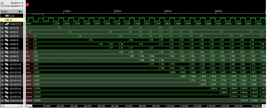
Figure 6.3: Data transition from Input to Output
The Non-Restoring algorithm implementation was synthesized using a 180 nm process
de-sign kit (PDK), results are shown in table6.1.
6.2
Restoring
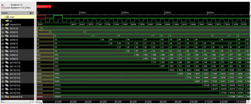
Cursor at TimeA and TimeB indicates that the clock period is 20 ns. The time taken to complete
[image:40.612.87.524.308.485.2]6.2 Restoring 30
[image:41.612.84.526.128.182.2]evaluates the 18 bit square root result in 18 clock cycles.
Figure 6.4: Pipeline Data flow for Restoring Algorithm
The square root of the first input is provided after 18 clock cycles. It is observable that
the next input to the square root computational block is evaluated before the completion of the
previous input evaluation by the system, thus indicating the operation of the 18 stage pipelined
system design. Compared to the non-pipelined implementation, which would consume 18 clock
cycles per input evaluation , it is can be observed that, once the pipeline is filled, the system is
able to process a new data every clock cycle ., the system consumes on an average 1 clock cycle
per input. The pipelining thus increases the throughput by over 17 times of the non-pipelined
implementation. The termination stage of the algorithm detects the polarity of the last partial
remainder and if required flip the last asserted quotient bit to 0.
[image:41.612.86.523.462.643.2]6.2 Restoring 31
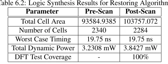
Table 6.2: Logic Synthesis Results for Restoring Algorithm
Parameter Pre-Scan Post-Scan
Total Cell Area 93584.9385 103757.072
Number of Cells 2340 2284
Worst Case Timing 19.75 ns 19.75 ns Total Dynamic Power 3.2308 mW 3.8427 mW
DFT Test Coverage - 100%
The Restoring algorithm implementation was synthesized using a 180 nm process design kit
Chapter 7
Conclusion
The objective of the paper was to design a high-throughput implementation of a square root
com-putational core. A restoring and non-restoring approaches were considered for the design of the
core. The square root computation was implemented as a 18-stage pipeline which increases the
throughput of the system by 17 times compared to the non-pipelined implementation. It was
observed that the non-restoring approach required fewer hardware components compared to the
restoring algorithm but required more control and branching functions compared to the later.
Hence, the choice between restoring and non-restoring is a trade-off between hardware cost and
system complexity. The restoring algorithm can be further simplified by combining the
remain-der restoration operation with the new remainremain-der computation. This would significantly reduce
the power consumption of the system by eliminating unnecessary signal transitions associated
with decision making based on data evaluated in the current execution cycle. The non-restoring
algorithm provides an accurate bit of the computed square root value per iterative stage. Thus,
the number of bits required would always correspond to the number of stages in the system. The
restoring algorithm returns a bit of the quotient which is checked only in the next stage of the
33
termination stage whose function is to identify if the determined quotient bit is correct and is in
compliance with the partial remainder obtained from the previous stage. Thus, an n-bit square
root computation using the restoring algorithm would require n+1 clock cycles for evaluation.
The described implementations have been verified using a SystemVerilog test bench which
generates random unconstrained vectors to test the operation of the restoring and non-restoring
algorithm. The square root reference model in the test bench which is used to determine the
ex-pected output value of the device under test and is generated from the standard Simulink library.
Using a reference model source reduced the possibility of wrong error detection and increased
the reliability of validation of the DUT. The implemented functional coverage ensured that all
possible inputs to the square root core have been evaluated before test is completed, ensuring that
the system operation is tested for all possible values in the input range. The implementation have
been synthesized in 180nm technology standard and a comparison of the two implementations
References
[1] Y. Z. X. Wang, Q. Ye, and S. Yang, “A new algorithm for designing square root calculators
based on fpga with pipeline technology,” in2009 Ninth International Conference on Hybrid
Intelligent Systems, vol. 1, Aug 2009, pp. 99–102.
[2] Y. Li and W. Chu, “A new non-restoring square root algorithm and its vlsi implementations,”
in Proceedings International Conference on Computer Design. VLSI in Computers and
Processors, Oct 1996, pp. 538–544.
[3] R. V. W. Putra, “A novel fixed-point square root algorithm and its digital hardware design,”
inInternational Conference on ICT for Smart Society, June 2013, pp. 1–4.
[4] R. G. Lyons, High-Speed Square Root Algorithms. Wiley-IEEE Press, 2012, pp.
243–250. [Online]. Available: http://ieeexplore.ieee.org.ezproxy.rit.edu/xpl/articleDetails.
jsp?arnumber=6241243
[5] A. Nanhe, G. Gawali, S. Ahire, and K. Sivasankaran, “Implementation of fixed and
float-ing point square root usfloat-ing nonrestorfloat-ing algorithm on fpga,” in International Journal of
Computer and Electrical Engineering, Vol. 5, No. 5, October 2013, vol. 3, Feb 2013, pp.
226–230.
fp-References 35
gas,” in Proceedings. The 5th Annual IEEE Symposium on Field-Programmable Custom
Computing Machines Cat. No.97TB100186), Apr 1997, pp. 226–232.
[7] A. Rahman and Abdullah-Al-Kafi, “New efficient hardware design methodology for
modi-fied non-restoring square root algorithm,” in2014 International Conference on Informatics,
Electronics Vision (ICIEV), May 2014, pp. 1–6.
[8] P. Kachhwal and B. C. Rout, “Novel square root algorithm and its fpga implementation,” in
2014 International Conference on Signal Propagation and Computer Technology (ICSPCT
2014), July 2014, pp. 158–162.
[9] I. Sajid, M. M. Ahmed, and S. G. Ziavras, “Pipelined implementation of fixed point square
root in fpga using modified non-restoring algorithm,” in 2010 The 2nd International
Con-ference on Computer and Automation Engineering (ICCAE), vol. 3, Feb 2010, pp. 226–230.
[10] S. Majerski, “Square-root algorithms for high-speed digital circuits,” in 1983 IEEE 6th
Symposium on Computer Arithmetic (ARITH), June 1983, pp. 99–102.
[11] P. Montuschi and P. M. Mezzalama, “Survey of square rooting algorithms,”IEE
Proceed-ings E - Computers and Digital Techniques, vol. 137, no. 1, pp. 31–40, Jan 1990.
[12] J. Bannur and A. Varma, “The vlsi implementation of a square root algorithm,” in 1985
IEEE 7th Symposium on Computer Arithmetic (ARITH), June 1985, pp. 159–165.
[13] M. D. Ercegovac, “On digit-by-digit methods for computing certain functions,” in 2007
Conference Record of the Forty-First Asilomar Conference on Signals, Systems and
Com-puters, Nov 2007, pp. 338–342.
[14] C. K. Piromsopa and P. Chongsatitvatana, “An fpga implementation of a fixed-point square
References 36
[15] Y. Li and W. Chu, “Parallel-array implementations of a non-restoring square root
algo-rithm,” in Proceedings International Conference on Computer Design VLSI in Computers
and Processors, Oct 1997, pp. 690–695.
[16] D. R. Llamocca-Obregon, “A core design to obtain square root based on a non-restoring
algorithm,” inProceedings XI Workshop IBERCHIP, 03 2005.
[17] E. L. Oberstar,Fixed-Point Representation & Fractional Math. Oberstar Consulting, 2007.
[18] K. N. Vijeyakumar, V. Sumathy, P. Vasakipriya, and A. D. Babu, “Fpga implementation
of low power high speed square root circuits,” in 2012 IEEE International Conference on
Computational Intelligence and Computing Research, Dec 2012, pp. 1–5.
[19] B. Yang, D. Wang, and L. Liu, “Complex division and square-root using cordic,” in2012
2nd International Conference on Consumer Electronics, Communications and Networks
(CECNet), April 2012, pp. 2464–2468.
[20] W. Chu and Y. Li, “Cost/performance tradeoff of n-select square root implementations,”
in Proceedings 5th Australasian Computer Architecture Conference. ACAC 2000 (Cat.
No.PR00512), 2000, pp. 9–16.
[21] IEEE,IEEEStd 1364 - 2005 IEEE Standard for Verilog Hardware Description Language,
IEEE Std. "IEEEStd 1364 - 2005", 04 2006.
[22] C. Spear and G. Tumbush,SystemVerilog for Verification, Third Edition: A Guide to
Learn-ing the Testbench Language Features. Springer Publishing Company, Incorporated, 2012.
[23] J. Bergeron, I. Books24x7, and Books24x7.com,Writing testbenches using SystemVerilog,
1st ed. New York: Springer Science & Business Media, 2006;2007;.
References 37
[25] S. Sutherland, S. Davidmann, and P. Flake,SystemVerilog for Design. Springer US, 2006.
[26] S. A. Wadekar, “A rt level verification method for soc designs,” in IEEE International
[Systems-on-Chip] SOC Conference, 2003. Proceedings., Sept 2003, pp. 29–32.
[27] S. Das, R. Mohanty, P. Dasgupta, and P. P. Chakrabarti, “Synthesis of system verilog
asser-tions,” inProceedings of the Design Automation Test in Europe Conference, vol. 2, March
2006, pp. 1–6.
[28] A. Shetty and D. H. Mahmoodi, System Verilog Testbench Tutorial Using Synopsys EDA
Tools. Nano-Electronics & Computing Research Center School of Engineering San
Appendix I
Source Code
I.1
Non-restoring Algorithm
I.1.1
Non-Restoring Algorithm Operation
1 / *
2 *
3 * D e s c r i p t i o n : Non−R e s t o r i n g A l g o r i t h m i m p l e m e n t a t i o n f o r
4 * S q u a r e−r o o t c o m p u t a t i o n f o r a s i n g l e s t a g e
5 *
6 * A u t h o r : Vyoma Sharma
7 *
8 * /
9 module S q r t S t a g e ( DI , QI , RI , DO, QO, RO) ;
10 p a r a m e t e r StageNum = 2 0 ;
I.1 Non-restoring Algorithm 39
12 i n p u t w i r e [ StageNum : 0 ] QI ;
13 i n p u t w i r e [ 2 * StageNum : 0 ] RI ;
14 o u t p u t w i r e [ 1 5 : 0 ] DO;
15 o u t p u t w i r e [ StageNum : 0 ] QO;
16 o u t p u t w i r e [ 2 * StageNum : 0 ] RO;
17 w i r e [ 2 * StageNum : 0 ] rte mp ;
18 w i r e c o n d i t i o n ;
19 a s s i g n r t e m p = { RI , DI [ 1 5 : 1 4 ] } ;
20 a s s i g n c o n d i t i o n = ( r t e m p >= { QI , 2 ’ b01 } ) ;
21 a s s i g n DO = { DI [ 1 3 : 0 ] , 2 ’ b00 } ;
22 a s s i g n RO = c o n d i t i o n ? r t e m p − { QI , 2 ’ b01 } : r t e m p ;
23 a s s i g n QO = c o n d i t i o n ? { QI , 1 ’ b1 } : { QI , 1 ’ b0 } ;
24 e n d m o d u l e / / SQRTNRST
I.1.2
Non-Restoring Algorithm with Pipeline architecture
1 / *
2 *
3 * D e s c r i p t i o n : Non−R e s t o r i n g A l g o r i t h m i m p l e m e n t a t i o n
4 * f o r S q u a r e−r o o t c o m p u t a t i o n w i t h p i p e l i n e a r c h i t e c t u r e
5 *
6 * A u t h o r : Vyoma Sharma
7 *
8 * /
9
I.1 Non-restoring Algorithm 40
11 module SQRTNRST (
12 c l k ,
13 r e s e t ,
14 D a t a I n ,
15 D a t a O u t ,
16 t e s t _ m o d e ,
17 s c a n _ i n 0 ,
18 s c a n _ e n ,
19 s c a n _ o u t 0
20 ) ;
21 i n p u t
22 r e s e t , / / s y s t e m r e s e t
23 c l k ; / / s y s t e m c l o c k
24 i n p u t
25 s c a n _ i n 0 , / / t e s t s c a n mode d a t a i n p u t
26 s c a n _ e n , / / t e s t s c a n mode e n a b l e
27 t e s t _ m o d e ; / / t e s t mode s e l e c t
28 o u t p u t
29 s c a n _ o u t 0 ; / / t e s t s c a n mode d a t a o u t p u t
30 i n p u t
31 w i r e [ 1 5 : 0 ] D a t a I n ;
32 o u t p u t
33 r e g [ 1 8 : 0 ] D a t a O u t ;
34 / / L o c a l I n t e r c o n n e c t D e f i n i t i o n s f o r S t a g e 1
I.1 Non-restoring Algorithm 41
36 r e g [ 2 : 0 ] RI1 ;
37 r e g [ 1 5 : 0 ] DI1 ;
38 w i r e [ 1 5 : 0 ] DO1 ;
39 w i r e [ 1 : 0 ] QO1 ;
40 w i r e [ 2 : 0 ] RO1 ;
41 / / L o c a l I n t e r c o n n e c t D e f i n i t i o n s f o r S t a g e 2
42 r e g [ 2 : 0 ] QI2 ;
43 r e g [ 4 : 0 ] RI2 ;
44 r e g [ 1 5 : 0 ] DI2 ;
45 w i r e [ 1 5 : 0 ] DO2 ;
46 w i r e [ 2 : 0 ] QO2 ;
47 w i r e [ 4 : 0 ] RO2 ;
48 / / L o c a l I n t e r c o n n e c t D e f i n i t i o n s f o r S t a g e 3
49 r e g [ 3 : 0 ] QI3 ;
50 r e g [ 6 : 0 ] RI3 ;
51 r e g [ 1 5 : 0 ] DI3 ;
52 w i r e [ 1 5 : 0 ] DO3 ;
53 w i r e [ 3 : 0 ] QO3 ;
54 w i r e [ 6 : 0 ] RO3 ;
55 / / L o c a l I n t e r c o n n e c t D e f i n i t i o n s f o r S t a g e 4
56 r e g [ 4 : 0 ] QI4 ;
57 r e g [ 8 : 0 ] RI4 ;
58 r e g [ 1 5 : 0 ] DI4 ;
59 w i r e [ 1 5 : 0 ] DO4 ;
I.1 Non-restoring Algorithm 42
61 w i r e [ 8 : 0 ] RO4 ;
62 / / L o c a l I n t e r c o n n e c t D e f i n i t i o n s f o r S t a g e 5
63 r e g [ 5 : 0 ] QI5 ;
64 r e g [ 1 0 : 0 ] RI5 ;
65 r e g [ 1 5 : 0 ] DI5 ;
66 w i r e [ 1 5 : 0 ] DO5 ;
67 w i r e [ 5 : 0 ] QO5 ;
68 w i r e [ 1 0 : 0 ] RO5 ;
69 / / L o c a l I n t e r c o n n e c t D e f i n i t i o n s f o r S t a g e 6
70 r e g [ 6 : 0 ] QI6 ;
71 r e g [ 1 2 : 0 ] RI6 ;
72 r e g [ 1 5 : 0 ] DI6 ;
73 w i r e [ 1 5 : 0 ] DO6 ;
74 w i r e [ 6 : 0 ] QO6 ;
75 w i r e [ 1 2 : 0 ] RO6 ;
76 / / L o c a l I n t e r c o n n e c t D e f i n i t i o n s f o r S t a g e 7
77 r e g [ 7 : 0 ] QI7 ;
78 r e g [ 1 4 : 0 ] RI7 ;
79 r e g [ 1 5 : 0 ] DI7 ;
80 w i r e [ 1 5 : 0 ] DO7 ;
81 w i r e [ 7 : 0 ] QO7 ;
82 w i r e [ 1 4 : 0 ] RO7 ;
83 / / L o c a l I n t e r c o n n e c t D e f i n i t i o n s f o r S t a g e 8
84 r e g [ 8 : 0 ] QI8 ;
I.1 Non-restoring Algorithm 43
86 r e g [ 1 5 : 0 ] DI8 ;
87 w i r e [ 1 5 : 0 ] DO8 ;
88 w i r e [ 8 : 0 ] QO8 ;
89 w i r e [ 1 6 : 0 ] RO8 ;
90 / / L o c a l I n t e r c o n n e c t D e f i n i t i o n s f o r S t a g e 9
91 r e g [ 9 : 0 ] QI9 ;
92 r e g [ 1 8 : 0 ] RI9 ;
93 r e g [ 1 5 : 0 ] DI9 ;
94 w i r e [ 1 5 : 0 ] DO9 ;
95 w i r e [ 9 : 0 ] QO9 ;
96 w i r e [ 1 8 : 0 ] RO9 ;
97 / / L o c a l I n t e r c o n n e c t D e f i n i t i o n s f o r S t a g e 10
98 r e g [ 1 0 : 0 ] QI10 ;
99 r e g [ 2 0 : 0 ] RI10 ;
100 r e g [ 1 5 : 0 ] DI10 ;
101 w i r e [ 1 5 : 0 ] DO10 ;
102 w i r e [ 1 0 : 0 ] QO10 ;
103 w i r e [ 2 0 : 0 ] RO10 ;
104 / / L o c a l I n t e r c o n n e c t D e f i n i t i o n s f o r S t a g e 11
105 r e g [ 1 1 : 0 ] QI11 ;
106 r e g [ 2 2 : 0 ] RI11 ;
107 r e g [ 1 5 : 0 ] DI11 ;
108 w i r e [ 1 5 : 0 ] DO11 ;
109 w i r e [ 1 1 : 0 ] QO11 ;
I.1 Non-restoring Algorithm 44
111 / / L o c a l I n t e r c o n n e c t D e f i n i t i o n s f o r S t a g e 12
112 r e g [ 1 2 : 0 ] QI12 ;
113 r e g [ 2 4 : 0 ] RI12 ;
114 r e g [ 1 5 : 0 ] DI12 ;
115 w i r e [ 1 5 : 0 ] DO12 ;
116 w i r e [ 1 2 : 0 ] QO12 ;
117 w i r e [ 2 4 : 0 ] RO12 ;
118 / / L o c a l I n t e r c o n n e c t D e f i n i t i o n s f o r S t a g e 13
119 r e g [ 1 3 : 0 ] QI13 ;
120 r e g [ 2 6 : 0 ] RI13 ;
121 r e g [ 1 5 : 0 ] DI13 ;
122 w i r e [ 1 5 : 0 ] DO13 ;
123 w i r e [ 1 3 : 0 ] QO13 ;
124 w i r e [ 2 6 : 0 ] RO13 ;
125 / / L o c a l I n t e r c o n n e c t D e f i n i t i o n s f o r S t a g e 14
126 r e g [ 1 4 : 0 ] QI14 ;
127 r e g [ 2 8 : 0 ] RI14 ;
128 r e g [ 1 5 : 0 ] DI14 ;
129 w i r e [ 1 5 : 0 ] DO14 ;
130 w i r e [ 1 4 : 0 ] QO14 ;
131 w i r e [ 2 8 : 0 ] RO14 ;
132 / / L o c a l I n t e r c o n n e c t D e f i n i t i o n s f o r S t a g e 15
133 r e g [ 1 5 : 0 ] QI15 ;
134 r e g [ 3 0 : 0 ] RI15 ;
I.1 Non-restoring Algorithm 45
136 w i r e [ 1 5 : 0 ] DO15 ;
137 w i r e [ 1 5 : 0 ] QO15 ;
138 w i r e [ 3 0 : 0 ] RO15 ;
139 / / L o c a l I n t e r c o n n e c t D e f i n i t i o n s f o r S t a g e 16
140 r e g [ 1 6 : 0 ] QI16 ;
141 r e g [ 3 2 : 0 ] RI16 ;
142 r e g [ 1 5 : 0 ] DI16 ;
143 w i r e [ 1 5 : 0 ] DO16 ;
144 w i r e [ 1 6 : 0 ] QO16 ;
145 w i r e [ 3 2 : 0 ] RO16 ;
146 / / L o c a l I n t e r c o n n e c t D e f i n i t i o n s f o r S t a g e 17
147 r e g [ 1 7 : 0 ] QI17 ;
148 r e g [ 3 4 : 0 ] RI17 ;
149 r e g [ 1 5 : 0 ] DI17 ;
150 w i r e [ 1 5 : 0 ] DO17 ;
151 w i r e [ 1 7 : 0 ] QO17 ;
152 w i r e [ 3 4 : 0 ] RO17 ;
153 / / L o c a l I n t e r c o n n e c t D e f i n i t i o n s f o r S t a g e 18
154 r e g [ 1 8 : 0 ] QI18 ;
155 r e g [ 3 6 : 0 ] RI18 ;
156 r e g [ 1 5 : 0 ] DI18 ;
157 w i r e [ 1 5 : 0 ] DO18 ;
158 w i r e [ 1 8 : 0 ] QO18 ;
159 w i r e [ 3 6 : 0 ] RO18 ;
I.1 Non-restoring Algorithm 46
161 . DI ( DI1 ) ,
162 . QI ( QI1 ) ,
163 . RI ( RI1 ) ,
164 . DO( DO1 ) ,
165 . QO( QO1 ) ,
166 . RO( RO1 ) ) ;
167 S q r t S t a g e # ( 2 ) S t a g e 2 (
168 . DI ( DI2 ) ,
169 . QI ( QI2 ) ,
170 . RI ( RI2 ) ,
171 . DO( DO2 ) ,
172 . QO( QO2 ) ,
173 . RO( RO2 ) ) ;
174 S q r t S t a g e # ( 3 ) S t a g e 3 (
175 . DI ( DI3 ) ,
176 . QI ( QI3 ) ,
177 . RI ( RI3 ) ,
178 . DO( DO3 ) ,
179 . QO( QO3 ) ,
180 . RO( RO3 ) ) ;
181 S q r t S t a g e # ( 4 ) S t a g e 4 (
182 . DI ( DI4 ) ,
183 . QI ( QI4 ) ,
184 . RI ( RI4 ) ,
I.1 Non-restoring Algorithm 47
186 . QO( QO4 ) ,
187 . RO( RO4 ) ) ;
188 S q r t S t a g e # ( 5 ) S t a g e 5 (
189 . DI ( DI5 ) ,
190 . QI ( QI5 ) ,
191 . RI ( RI5 ) ,
192 . DO( DO5 ) ,
193 . QO( QO5 ) ,
194 . RO( RO5 ) ) ;
195 S q r t S t a g e # ( 6 ) S t a g e 6 (
196 . DI ( DI6 ) ,
197 . QI ( QI6 ) ,
198 . RI ( RI6 ) ,
199 . DO( DO6 ) ,
200 . QO( QO6 ) ,
201 . RO( RO6 ) ) ;
202 S q r t S t a g e # ( 7 ) S t a g e 7 (
203 . DI ( DI7 ) ,
204 . QI ( QI7 ) ,
205 . RI ( RI7 ) ,
206 . DO( DO7 ) ,
207 . QO( QO7 ) ,
208 . RO( RO7 ) ) ;
209 S q r t S t a g e # ( 8 ) S t a g e 8 (
I.1 Non-restoring Algorithm 48
211 . QI ( QI8 ) ,
212 . RI ( RI8 ) ,
213 . DO( DO8 ) ,
214 . QO( QO8 ) ,
215 . RO( RO8 ) ) ;
216 S q r t S t a g e # ( 9 ) S t a g e 9 (
217 . DI ( DI9 ) ,
218 . QI ( QI9 ) ,
219 . RI ( RI9 ) ,
220 . DO( DO9 ) ,
221 . QO( QO9 ) ,
222 . RO( RO9 ) ) ;
223 S q r t S t a g e # ( 1 0 ) S t a g e 1 0 (
224 . DI ( DI10 ) ,
225 . QI ( QI10 ) ,
226 . RI ( RI10 ) ,
227 . DO( DO10 ) ,
228 . QO( QO10 ) ,
229 . RO( RO10 ) ) ;
230 S q r t S t a g e # ( 1 1 ) S t a g e 1 1 (
231 . DI ( DI11 ) ,
232 . QI ( QI11 ) ,
233 . RI ( RI11 ) ,
234 . DO( DO11 ) ,
I.1 Non-restoring Algorithm 49
236 . RO( RO11 ) ) ;
237 S q r t S t a g e # ( 1 2 ) S t a g e 1 2 (
238 . DI ( DI12 ) ,
239 . QI ( QI12 ) ,
240 . RI ( RI12 ) ,
241 . DO( DO12 ) ,
242 . QO( QO12 ) ,
243 . RO( RO12 ) ) ;
244 S q r t S t a g e # ( 1 3 ) S t a g e 1 3 (
245 . DI ( DI13 ) ,
246 . QI ( QI13 ) ,
247 . RI ( RI13 ) ,
248 . DO( DO13 ) ,
249 . QO( QO13 ) ,
250 . RO( RO13 ) ) ;
251 S q r t S t a g e # ( 1 4 ) S t a g e 1 4 (
252 . DI ( DI14 ) ,
253 . QI ( QI14 ) ,
254 . RI ( RI14 ) ,
255 . DO( DO14 ) ,
256 . QO( QO14 ) ,
257 . RO( RO14 ) ) ;
258 S q r t S t a g e # ( 1 5 ) S t a g e 1 5 (
259 . DI ( DI15 ) ,
I.1 Non-restoring Algorithm 50
261 . RI ( RI15 ) ,
262 . DO( DO15 ) ,
263 . QO( QO15 ) ,
264 . RO( RO15 ) ) ;
265 S q r t S t a g e # ( 1 6 ) S t a g e 1 6 (
266 . DI ( DI16 ) ,
267 . QI ( QI16 ) ,
268 . RI ( RI16 ) ,
269 . DO( DO16 ) ,
270 . QO( QO16 ) ,
271 . RO( RO16 ) ) ;
272 S q r t S t a g e # ( 1 7 ) S t a g e 1 7 (
273 . DI ( DI17 ) ,
274 . QI ( QI17 ) ,
275 . RI ( RI17 ) ,
276 . DO( DO17 ) ,
277 . QO( QO17 ) ,
278 . RO( RO17 ) ) ;
279 S q r t S t a g e # ( 1 8 ) S t a g e 1 8 (
280 . DI ( DI18 ) ,
281 . QI ( QI18 ) ,
282 . RI ( RI18 ) ,
283 . DO( DO18 ) ,
284 . QO( QO18 ) ,
I.1 Non-restoring Algorithm 51
286 a l w a y s @( p o s e d g e c l k , p o s e d g e r e s e t ) b e g i n
287 i f ( r e s e t == 1 ’ b1 ) b e g i n 288 D a t a O u t <= 0 ;
289 QI1 <= ’ b0 ;
290 RI1 <= ’ b0 ;
291 DI1 <= ’ b0 ;
292 DI2 <= ’ b0 ;
293 QI2 <= ’ b0 ; / / Q u o t i e n t I n p u t
294 RI2 <= ’ b0 ; / / R e m a i n d e r I n p u t
295 QI3 <= ’ b0 ;
296 RI3 <= ’ b0 ;
297 DI3 <= ’ b0 ;
298 QI4 <= ’ b0 ;
299 RI4 <= ’ b0 ;
300 DI4 <= ’ b0 ;
301 QI5 <= ’ b0 ;
302 RI5 <= ’ b0 ;
303 DI5 <= ’ b0 ;
304 QI6 <= ’ b0 ;
305 RI6 <= ’ b0 ;
306 DI6 <= ’ b0 ;
307 QI7 <= ’ b0 ;
308 RI7 <= ’ b0 ;
309 DI7 <= ’ b0 ;
I.1 Non-restoring Algorithm 52
311 RI8 <= ’ b0 ;
312 DI8 <= ’ b0 ;
313 QI9 <= ’ b0 ;
314 RI9 <= ’ b0 ;
315 DI9 <= ’ b0 ;
316 QI10 <= ’ b0 ;
317 RI10 <= ’ b0 ;
318 DI10 <= ’ b0 ;
319 QI11 <= ’ b0 ;
320 RI11 <= ’ b0 ;
321 DI11 <= ’ b0 ;
322 QI12 <= ’ b0 ;
323 RI12 <= ’ b0 ;
324 DI12 <= ’ b0 ;
325 QI13 <= ’ b0 ;
326 RI13 <= ’ b0 ;
327 DI13 <= ’ b0 ;
328 QI14 <= ’ b0 ;
329 RI14 <= ’ b0 ;
330 DI14 <= ’ b0 ;
331 QI15 <= ’ b0 ;
332 RI15 <= ’ b0 ;