A BEC Based Precision Gravimeter and Magnetic Gradiometer: Design and Implementation

(1)

A BEC Based Precision Gravimeter and

Magnetic Gradiometer:

Design and Implementation

Kyle S. Hardman

A thesis submitted in partial fulfilment of the requirements for the degree of

Doctor of Philosophy in Physicsat the Australian National University

(2)

(3)

iii

A BEC Based Precision Gravimeter and

Magnetic Gradiometer:

Design and Implementation

Kyle S. Hardman

Department of Quantum Science The Australian National University

Supervisory committee: Professor Nicholas P. Robins (Chair) Professor John D. Close

Professor Joseph J. Hope

Abstract

A precision inertial sensor based on the interference of matter waves has been designed and implemented. The apparatus is capable of producing both cold thermal and ultra-cold Bose-Einstein condensate (BEC) atomic ensembles as the inertial test mass. BECs of up to 5×106 Rubidium 87 atoms with an effective temperature (Te f f) of 50 nK are

produced every 13 seconds using a combination of two and three dimensional magneto-optical traps (2D and 3D MOT) and evaporative cooling in a hybrid magnetic-quadrupole and crossed optical dipole trap. The atomic cloud is then propagated through a ver-tically oriented Mach-Zehnder interferometer utilizing Bragg diffraction beam splitters. An∼2.6 m drop tube allows for up to 750 ms of free fall and interferometer times (T) of up to∼250 ms. The drop has four regions of imaging corresponding to 0−25 ms, 220 ms, 530 ms, and 750 ms of expansion. Standard absorption imaging is used for the upper two imaging regions and frequency modulation imaging (FMI) is used for the lower re-gions. FMI exhibits near atom-shot noise limited signal-to-noise of ∼948 on a 1×106 atom cloud. The inertial reference is provided by the Bragg beam retroreflector which is suspended via a geometric anti-spring passive vibration isolation system providing 65 dB of isolation at 70 Hz. Prior to the first interferometer pulse the ensemble is placed into a spin superposition of the|F=1iground state manifold using horizontal co-propagating Raman beams. The three internal spin states remain orthogonal throughout the interfer-ometer sequence resulting in three simultaneous interferinterfer-ometer with separable magnetic gradient and gravitational acceleration signals.

(4)

is below 1 mrad. No significant decrease in the interferometer contrast is observed for all available T, whereas a thermal test mass interferometer of equivalent longitudinal temperature produces no interference atT>100 ms.

A direct comparison of test mass spatial coherence length in an optically transversely confined interferometer is investigated. The visibility and contrast of a BEC and three thermal sources with varying spatial coherence are compared as a function of interfer-ometer time. At short times, the fringe visibility of a BEC source approaches 100 %, nearly independent of π pulse efficiency, while thermal sources have fringe visibilities limited to theπ pulse efficiency. More importantly for precision measurement systems, the BEC source maintains interference at interferometer times significantly beyond that of the thermal source.

A BEC test mass is used for the simultaneous precision measurement of gravity and magnetic field gradients. An 8 hour data run of aT=130 ms interferometer shows good agreement between the interferometer output and a theoretical model of the solid earth tides. The residual of the theoretical model and the experimental data show a 1000 run precision of∆g/g = 1.45×10−9corresponding to a phase noise of ∼3.8 mrad. The in-tegrated phase noise of the apparatus shows a sensitivity to magnetic field gradients of 120 pT/m. By varying the central spatial position of aT =40 ms interferometer the mag-netic field gradient along a portion of the drop tube is measured.

Declaration

To the best of my knowledge and except where acknowledged in the customary manner, the material presented in this thesis is original and has not been submitted in whole or part for a degree in any university. Where work has been performed in collaboration with others, I have acknowledged the contributions of all authors.

(5)

Acknowledgments

Firstly, I would like to express my gratitude for my adviser, Nick Robins. Without his willingness to bring me to Australia and give me all but free reign to build up a brand new lab none of this would have been possible. His advice, knowledge, and friendship have been invaluable during the last five years and I am very thankful for this.

I would like to thank John Close for tirelessly working to bring funding into the lab so that my colleagues and I were never in a situation where scientific progress hindered. Our candid discussions about politics and physics have really helped keep me entertained.

For my fellow group members JD, Carlos, Gordon, Paul, Manju, Patrick, Mahasen, and Ciaron: thank you for making this a fun and entertaining group to be a part of. The last five years would not have gone by quite as fast or been remotely as successful without the relationships and discussions I have had with all of you. Kyle10 would not exist without your help. I want you all to remember that no matter how challenging things get, experimental physics isn’t hard; it’s just tedious.

To Aunt Cathy and Uncle Mark: thank you for giving me a home away from home during my time in Australia. It was a great comfort having family so close.

I am very grateful for Michelle. Her support and understanding during the full weeks and long hours over the last five years has been nothing short of amazing. I could not ask for a better or more caring partner.

Finally, I would like to thank my sister and parents. I could not have had a better sister to grow up with than Rose. Her dedication to pursue the things that she is most passionate about has been an inspiration. I am so proud of all her accomplishments. My parents Dennis and Nancy have always encouraged me to pursue any and every avenue I have chosen to take in life. Their unwavering support and interest has given me a unique advantage to succeed in all aspects of both my professional and personal life, from sports to academia to relationships. I cannot express strongly enough how thankful I am to have had them shape my life.

(6)

(7)

List of Publications

• G. D. McDonald, H. Keal, P. A. Altin, J. E. Debs, S. Bennetts, C. C. N. Kuhn, K. S. Hardman, M. T.

Johnsson, J. D. Close, and N. P. Robins. Optically guided linear mach-zehnder atom interferometer.

Phys. Rev. A87, 013632 (2013).DOI:10.1103/PhysRevA.87.013632. [pp 114, 117]

• P. A. Altin, M. T. Johnsson, V. Negnevitsky, G. R. Dennis, R. P. Anderson, J. E. Debs, S. S. Szigeti,

K. S. Hardman, S. Bennetts, G. D. McDonald, L. D. Turner, J. D. Close, and N. P. Robins.Precision

atomic gravimeter based on bragg diffraction. New Journal of Physics15, 023009 (2013). [p 65]

• J. E. Debs, K. S. Hardman, P. A. Altin, G. D. McDonald, J. D. Close, and N. P. Robins.From apples

to atoms: measuring gravity with ultra cold atomic test masses. Preview (2013).

• G. D. McDonald, C. C. N. Kuhn, S. Bennetts, J. E. Debs, K. S. Hardman, M. Johnsson, J. D.

Close, and N. P. Robins. 80¯hk momentum separation with bloch oscillations in an optically guided

atom interferometer. Phys. Rev. A88, 053620 (2013). DOI:10.1103/PhysRevA.88.053620. [pp 114, 118, and 136]

• C. C. N. Kuhn, G. D. McDonald, K. S. Hardman, S. Bennetts, P. J. Everitt, P. A. Altin, J. E.

Debs, J. D. Close, and N. P. Robins. A bose-condensed, simultaneous dual-species mach–zehnder

atom interferometer. New Journal of Physics16, 073035 (2014). [p 114]

• K. S. Hardman, C. C. N. Kuhn, G. D. McDonald, J. E. Debs, S. Bennetts, J. D. Close, and

N. P. Robins. Role of source coherence in atom interferometry. Phys. Rev. A89, 023626 (2014).

DOI:10.1103/PhysRevA.89.023626. [pp 3, 113]

• G. D. McDonald, C. C. N. Kuhn, S. Bennetts, J. E. Debs, K. S. Hardman, J. D. Close, and N. P.

Robins. A faster scaling in acceleration-sensitive atom interferometers. EPL (Europhysics Letters)

105, 63001 (2014).

• K. S. Hardman, S. Bennetts, J. E. Debs, C. C. N. Kuhn, G. D. McDonald, and N. Robins.

Con-struction and Characterization of External Cavity Diode Lasers for Atomic Physics. JOVE (Journal of

Visualized Experiments) page e51184 (2014). ISSN 1940-087X. DOI:10.3791/51184.

• S. Bennetts, G. D. McDonald, K. S. Hardman, J. E. Debs, C. C. N. Kuhn, J. D. Close, and N. P.

Robins. External cavity diode lasers with 5khz linewidth and 200nm tuning range at 1.55µm and

methods for linewidth measurement. Opt. Express22, 10642 (2014). DOI:10.1364/OE.22.010642. [pp 38, 39]

• G. D. McDonald, C. C. N. Kuhn, K. S. Hardman, S. Bennetts, P. J. Everitt, P. A. Altin, J. E. Debs,

J. D. Close, and N. P. Robins. Bright solitonic matter-wave interferometer. Phys. Rev. Lett.113,

013002 (2014). DOI:10.1103/PhysRevLett.113.013002.

• P. B. Wigley, P. J. Everitt, A. van den Hengel, J. W. Bastian, M. A. Sooriyabandara, G. D.

McDon-ald, K. S. Hardman, C. D. Quinlivan, P. Manju, C. C. N. Kuhn, I. R. Petersen, A. N. Luiten, J. J.

Hope, N. P. Robins, and M. R. Hush. Fast machine-learning online optimization of ultra-cold-atom

experiments. Scientific Reports6, 25890 (2016).

(8)

• K. S. Hardman, P. J. Everitt, G. D. McDonald, P. Manju, P. B. Wigley, M. A. Sooriyabandara,

C. C. N. Kuhn, J. E. Debs, J. D. Close, and N. P. Robins. Simultaneous precision gravimetry and

magnetic gradiometry with a bose-einstein condensate: A high precision, quantum sensor. Phys. Rev. Lett.117, 138501 (2016).DOI:10.1103/PhysRevLett.117.138501. [pp 3, 123]

• P. B. Wigley, P. J. Everitt, K. S. Hardman, M. R. Hush, C. H. Wei, M. A. Sooriyabandara, P. Manju,

J. D. Close, N. P. Robins, and C. C. N. Kuhn. Non-destructive shadowgraph imaging of ultra-cold

(9)

Introduction

T

HE quest for an understanding of gravitation has spanned hundreds of years and billions of light years, from the early experiments of Simon Stevin in 1586 demon-strating the equivalence of free fall [1] and Sir Issac Newton’s formulation of the inverse square law [2] to the discovery of the Higgs boson in 2012 [3] and the measurement of gravitational waves produced by orbiting black holes 1.3 billion light years away from earth [4]. The contributions of these endeavors to the advancement in understanding the mechanics of the universe can not be overstated. However, as we continue to look out-wards in search of what gravitation may reveal about the universe it is also important to ask what gravitation may be able to uncover about the Earth itself.

The underlying principle of gravitation is illustrated by Newton’s universal law of gravitation 1.1 whereF is force, m1,2 anda1,2 are mass and acceleration of object 1 and

2 respectively, andr the distance between the masses. This simple equation describes the classical attraction between massive bodies and shows a direct relation between the absolute acceleration of a test mass (a1,2) and the total mass (m2,1) acting on it.

F= m1,2a1,2=

Gm1m2

r2 (1.1)

With this relation and the development of high precision gravity sensors it has become possible to explore the spatial and temporal gravitational dynamics of the Earth with unprecedented accuracy.

g = 9.7959938810 m/s

2

Aquifers

Altitude Tides Air Pressure

Solid Density Glacial Rebound

Figure 1.1: A general value of gravitational acceleration (g). The maximum deviation from this

value for various sources is highlighted. Note: Adapted from a presentation by Richard Lane of

Geo-science Australia.

Through the precise monitoring of local gravitational acceleration it is possible to identify time dependent changes in gravity from a number of sources, such as altitude changes, the Earth-moon-sun orbital system (tidal forces), variations in atmospheric air pressure, the filling and draining of subterranean aquifers, or ground uplift caused from glacial rebound. Additionally, with the advent of portable sensors, spatial anomalies in the Earth’s crust caused by changes in the solid earth density can be observed. The ability to measure these signals is critical to the many scientific fields including mineral and oil exploration and monitoring [5, 6], water reserve discovery and monitoring [7], climate

(14)

Gravimeter Type Precision ∆_gg Accuracy (g)

Scintrex Autograv CG-5 Spring-mass

(Relative) <5×10

−9_[25] _N/A

GWR Instruments iOSG

Superconducting Mass Levitation

(Relative)

1×10−12[26] N/A

Micro-g LaCoste FG5-X Falling Corner-cube

(Absolute) 1×10

−10_[27] ₂_×₁₀−9_[27]

GAIN Falling Atom Cloud

(Absolute) 5×10

−11_[24] _3.9_×₁₀−9_[24]

Table 1.1: Performance of various gravity meters.

science [8], and navigation based on gravity maps [9]. Figure 1.1 shows the change in gravitational acceleration from various spatial and temporal features [7, 10].

In response to the vast applications of precision gravimetry a diverse array of devices have been developed to directly measure (absolute) or measure changes (relative) to the relation in Equation 1.1 to high precision. The most notable of the early sensors are based off macroscopic classical springs [11], super conducting systems [12], and falling corner cubes [13]. Following early pioneering work in precision atom interferometry [14], the past decade has seen devices using cold atomic sources become competitive with tradi-tional gravitation sensors [15, 16, 17, 18, 19]. Table 1.1 shows the highest achieved inte-grated sensitivities achieved by various sensors as well as the accuracy achieved by sen-sors capable of the absolute measurement ofg. Technical developments improving size, weight and power have allowed for applications in space science [20] and field ready state-of-the-art gravimeters and gradiometers [21, 22, 23, 24].

Supplementing gravitational anomaly data with other quantities such as magnetic field gradients (∆Bz) has the potential to improve mapping resolution as well as enhance

the ability to identify specific materials based on their magnetic and density signatures [28]. Ferromagnetic, paramagnetic, and diamagnetic features from an array of mineral deposits and water reservoirs cause large variations in the Earth’s natural magnetic field gradient. The maximum expected gradients at a 100 m measuring distance resulting from a number of magnetic features is shown in Figure 1.2.

= 0000.002709 nT/m

Iron Ore Ma�ic-Felsic Gneiss Vertical Contact

Magnetite Felsic Gneiss

dz

dB

Figure 1.2: A general value of Earth’s background vertical magnetic field gradient (∆Bz). The

maximum deviation from this value for various sources is highlighted.

(15)

Introduction 3

Magnetic Gradiometer Type Precision (∆Bz)

Fluxgate Solid-state 520 pT/m [29]

SQUID

Superconducting Quantum Interference

10 pT/m [30]

ANU Atom Interferometer

Falling Atom

Cloud 120 pT/m [31]

Table 1.2: Performance

of various magnetic

gradient meters.

Recent efforts have been made to combined magnetic and gravitational data to im-prove feature recognition [32] however, the inability to acquire the data under identi-cal conditions (simultaneously) does not allow effective stitching of the two data sets. Furthermore having to run multiple data acquisition campaigns greatly increases explo-ration costs, especially for airborne measurements.

Atom based systems have previously been shown to outperform all absolute gravity meters [24] as well as shown promise for the precision detection of magnetic field gradi-ents [33]. The ability to access internal degrees of freedom in atom based sensors allows for the system to exhibit deterministic responses to select fields. By operating these sen-sors in a mix of internal states it is then possible to simultaneously measure various back-ground quantities. Additionally, atom interferometers rely on a sequence of laser pulses to split and redirect the atomic sample through the interferometer. The laser pulses are analogus to optical mirrors and beam splitters in typical optical interferometers. This fea-ture allows for the dynamic control of interferometer configurations simply by changing the type and sequence of pulses. It is possible to make the interferometer sensitive to different quantities such as gravitational fields and their gradients [15], rotations [34, 35], or time [36]. Although these advantages are intrinsic to all atomic sources, ultra-cold Bose-Einstein condensates (BEC) offer additional benefits over thermal atoms. An intrin-sic feature of a BEC is a spatial coherence equivalent to the size of the cloud which is generally 100s ofµm while thermal sources have spatial coherence length on the order of the de Broglie wavelength typically∼0.1µm. This spatial coherence is shown to provide robustness to systematics which result in loss of fringe contrast such as cloud mismatch at the final beam splitter pulse [37, 38]. The BEC then allows a sensor to be operated un-shielded in varying environments where background field gradients and curvatures are non-negligible.

(16)

1.1 Atom Interferometry

The atom interferometer is the matter-wave analog to the well known optical interfer-ometer. As a consequence of the wave-particle duality of matter, all massive objects may be represented as a wave function (|Ψi) with deterministic frequency (ω) and phase (φ) [39]. This property allows for the propagation of a matter-wave interferometer where light and matter have exchanged roles. Just like their optical counterparts, atom inter-ferometers rely on placing a single input source into a superposition of two states which propagate through different interferometer arms, acquiring relative phase, before being recombined and hence interfered. This is accomplished using optical mirrors and beam splitters in optical interferometers and pulses of an optical lattice in a matter-wave inter-ferometer.

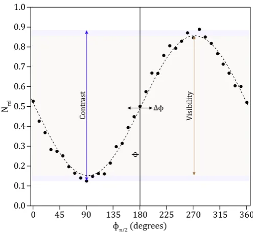
While optical beam paths are separated in position space matter-wave inertial sensors operate with momentum space superpositions. The amplitude of each recombined state is then measured. By comparing the amplitude of the output states the relative phase between the two interferometer paths can be acquired. The output state amplitudes are found by counting the number of atoms in each state. This can be accomplished using absorption imaging (AI), fluorescence imaging (FI), or frequency modulation imaging (FMI), a newly implemented technique used in this research. These three imaging tech-niques are discussed in Sections 5.1, 5.2, and 5.3. Much like an optical interferometer, an interferometric fringe may be scanned by varying the relative path length of the interfer-ometer arms. In optical systems this is accomplished by directly adjusting a beam path by simply modulating the position of a mirror or beam splitter. Similarly, a fringe may be traced in a matter-wave interferometer by scanning the optical phase of the lattice, as will be seen in the derivation of the atom interferometer phase relation. An example of an interferometric fringe from a atom interferometer is shown in Figure 1.3, where the normalized atom number (N_rel = N1/(N1+N2), where N1,2 are the atom numbers in

output states|1, 2i, respectively) in output state 1 (|1i) is plotted as the optical phase of the lattice is scanned through 360◦. Figures of merit for an interferometer fringe are as follows: contrast (C), the maximum deviation in N_rel; visibility (V), the amplitude of a sinusoidal fit to the fringe; phase (φ), the absolute phase of the sinusoidal fit; and phase uncertainty (∆φ), the standard deviation inφof the sinusoidal fit. It should be noted that contrast is a quantitative measure of the interference strength but does not imply phase sensitivity as it is possible to have high fringe contrast while ∆φ > πrad. A non-zero measurement of visibility is only possible for interferometers which exhibit measurable φimplying sensitivity to changes in the interferometer propagation.

As stated above, the splitting, redirecting, and recombining of the atomic sample in precision inertial sensors is generally realized using pulses of an optical lattice formed by mutually polarized counter propagating beams of wave numbersk1 andk2(ki = 2π/λi,

where λi is the wavelength of the ith beam). A common variable which will be used

(17)

Introduction 5

Nrel 0.9 0.8 0.7 0.6 0.5 0.4 0.3

0.2 0.1

135 90 45 0

фπ/2 (degrees)

180 225 270 315 360 0.0

1.0

Contr

ast

Visibility

∆φ

[image:17.595.101.349.89.316.2]

φ

Figure 1.3: Example of a atom inter-ferometer fringe taken by scanning the effective phase of one of the

lat-tice pulses. (—) The interferometer

contrast as given by the maximum deviation in Nrel = N1/(N1+N2),

where N1,2 are the atom numbers in

output states|1, 2i, respectively. (—

) The interferometer visibility given by 2 times the amplitude of a sinu-soidal fit to the fringe. (—) The

inter-ferometer phase (φ) and uncertainty

in phase (∆φ) as determined from the sinusoidal fit.

a momentum difference but also an internal energy difference between the two interfer-ometer arms. The difference in internal energies ensures that no free propagation time is needed for the states to spatially separate prior to imaging, as the two ports’ imaging transitions are non-degenerate. Raman pulsed interferometers are more susceptible to ac-Stark and Zeeman shifts, which affect the two interferometer arms differently due to the internal state difference. This will negatively contribute to the interferometer phase par-ticularly in unshielded environments. Conversely, Bragg based interferometers are first order insensitive to these environmental effects but require spatial separation of the two output states in order to image. Additionally, the Bragg transition frequency typically ranges from 10s of kHz to 10s of MHz while Raman transitions between hyperfine levels can be∼10 GHz. The relatively low frequency of the Bragg transitions greatly simplifies the electronics needed to control the laser frequencies.

There are a number of common configurations for atom interferometers including the Ramsey-Bordé, butterfly, and Mach-Zehnder all with different phase dependencies. For the purposes of this thesis only the Mach-Zehnder interferometer (MZI) will be discussed as it exhibits behavior conducive to inertial sensing.

The typical MZI is made up of three Bragg pulses: the first pulse at timeT0places the

initial cloud into a 50/50 (π/2 pulse) superposition of two momentum states (|1, 2i); the two states are allowed to propagate forTbefore a second pulse mirrors the momentum states (π pulse) such that the momentum of |1iis now the momentum of|2iand vice versa; lastly, the states propagate for another timeT after which a third and final Bragg pulse (π/2 pulse) is applied, mixing and interfering the two arms. An illustration of a MZI propagating in an inertial field is shown in Figure 1.4. Throughout this thesisTwill be referred to as the interferometer time. The definition of the notedπandπ/2 pulses are a result of specific conditions during the Rabi flopping of a two-level transition, discussed in Section 4.1.

(18)

k1 k1

k2 k2

|1

ag

T T

ф1

ф2

k1

k2

ф3 |2

|1 |2 aB

Figure 1.4: Illustration of an atomic sourced Mach-Zehnder interferometer (MZI).

action along each interferometer path [10]. In the limit where the internal clocks of each interferometer arm (ω1,2) tick at the same rate Equation 1.2 is found, showing a direct

relation between the acceleration of the atoms (a), the lattice phase (φL), and the

interfer-ometer phase (φ). This thesis will continually reference Equation 1.2 as it, and variations on it, fully describe the phase behavior of the interferometer.

φ=k_{e f f}aT2+φL (1.2)

Under conditions in which the internal clock rates are not identical a phase term must be added corresponding to the difference in the accumulated phase attributed to the un-equal clock rates, as shown in Equation 1.3. Differences in clock rates may arise from a number of sources including gravitational redshift [44, 45, 46, 47] and, key to this appa-ratus, internal energy variations between the atomic ensembles caused by the meanfield energy of the Bose-condensed source [48, 49]. The effects of this meanfield energy in the interferometer are theoretically and experimentally explored in Section 7.6.

φc =

Z 2T 0

(ω₁−ω2)dt (1.3)

As with all inertial measurements, the measurement must be measured in relation to some absolute reference. As such it should be noted that the acceleration in Equation 1.2 is the relative acceleration between the propagating atom cloud and the lattice laser. Vibrations which modulate the phase of the lattice then directly couple to the interferom-eter in a way that is indistinguishable from pure acceleration of the atom cloud. Great care is then taken to provide a system which effectively eliminates background vibrations that couple to the lattice, described in detail in Section 6.

1 2

V √

N = ke f f∆aT

2 _(1.4)

(19)

Chapter 2

Vacuum System

Figure 2.1: Rendered draw-ing of the designed vacuum system.

In order to facilitate effective cooling during all steps of the cooling procedure the atomic ensemble’s interaction with the 300 K environment must be limited. Three main ther-mal energy transportation mechanisms must be considered when attempting to isolate the atoms: radiative; mechan-ical; and convective. Radiative heating of cooled samples is of tremendous concern and requires extensive radiation shielding when considering bulk objects like those seen in cryogenic buffer gas systems [50]. However, the low den-sity laser cooled atomic samples used in this apparatus have vanishingly small photon absorption cross-sections and rel-atively limited atomic transitions in comparison. These two properties alone all but eliminate any heating effect from black-body radiation. In order to eliminate or at least re-duce the heating effects caused by mechanical and convec-tive processes to tolerable levels the atomic sample may be placed in an ultra-high vacuum (UHV) chamber and iso-lated from the walls using various optical and magnetic techniques. The techniques used for trapping the atomic en-semble are discussed in Section 3. Sections 2.2 and 2.3 dis-cusses the mechanical and convective heating mechanisms, while the vacuum system design is detailed in Section 2.4.

2.1 Radiative Heating

The absorption and emission of radiation from bulk objects of finite temperature is described by Planck’s law which is given in Equation 2.1, wherehis Planck’s constant,cis the speed of light, A is the area of the object, λ is the wave-length of light, kB is Boltzmann’s constant, and Te f f is the

object’s temperature. This expression well defines the ra-diation spectrum of systems which behave as black-body radiators such as the vacuum system walls. For a typical black-body absorber atT_{e f f} = 0 being irradiated by a 300 K source the total absorbed power is given by the integration of Equation 2.1 across allλ.

(20)

P=2hcA

Z ₁

λ5

e

hc kBTe f fλ ₋

1

−1

dλ (2.1)

To estimate the amount of power absorbed by an atomic sample the quantized ab-sorption spectrum must be considered. The total power available to be absorbed by the atomic sample, to a good approximation, is given by integrating Equation 2.1 across the individual atomic absorption lines using their respective linewidths. For the87Rbsample used here there exist only two fine-structure transitions with λ < 50µatλ0 ≈ 780 nm

and 795 nm. Using the on resonant absorption cross-section as given by 3λ2₀/2πthe esti-mated absorbed power per atom from the 300 K background is∼2×10−41W. This power corresponds to a single photon absorption event in∼4×1014years leading to a negligible heating rate caused by black-body radiation.

2.2 Mechanical Heating

Mechanical heating is caused by the transfer of heat through solid mechanically linked objects of different temperatures. Generally, the rate of heat exchange between ridgedly connected objects is given by Equation 2.2, where κ is the thermal conductivity of the interface,∆T_{e f f} is the temperature difference between the objects,Ais the cross-section, andxis the length of the interface. By levitating the atomic sample using optical and/or magnetic fields any structural connection between the 300 K environment and the sample is eliminated.

γheat =κ∆Te f f

A

x (2.2)

2.3 Convective Heating and Atom Loss

The most pressing concern when considering the interactions of trapped atomic sources with the 300 K environment is collisions of the sample with hot background gasses. These collisions lead to heating as well as loss of atoms from the atomic ensemble. The formula-tion and dynamics of the interacformula-tions has been explored in previous works and therefore will only be discussed briefly here [51, 52].

The background pressure of UHV systems is generally dominated by diatomic Hy-drogen molecules (H2) and can be checked fairly simply through the use of a mass

spec-trum analyzer. Due to the relatively low temperature of the cooled atoms compared to the background gas the inter-atomic velocity is dominated by the 300 K background gas. The elastic scattering rate between the cold trapped atoms and the hot background gas is given by Equation 2.3, where N is the number of trapped atoms, nb is the

den-sity of the background gas, vb is the velocity of the background gas as given by vb =

q

3kbTe f f/mb, mb is the mass of the dominant background species, and σatom is the

to-tal elastic cross-section comprised of classical and diffractive components between the colliding species. For theRb−H2collisions of interest hereσatom=295×10−20m2[51].

γscat=1.05Nnbvbσatom (2.3)

(21)

Vacuum System 9

The diffractive scattering limit is defined by the inequality in Equation 2.4, whereU is the depth of the trapping potential,e_d is the diffractive depth, ¯h is the reduced Planck’s constant, andmis the mass of the trapped atoms. To convert Equation 2.4 to tempera-ture simply divide bykB. Typical optical and magnetic traps used in atomic physics are

capable of trapping atoms ofT_{e f f} ≤ 1 mK which is small compared to thee_d = 23.6 mK for this system. The trapping potentials used here are discussed in Section 3.2.2.

U<e_d = 4π¯h

2

mσatom

(2.4)

In the diffractive scattering limit (shallow trap) the heating rate is then described by Equation 2.5 and the trap loss rate is effectively given by Equation 2.3. By reducing the background pressure (1×10−10Torr) and thereforenbthe heating and loss of atoms can

be reduced to manageable levels over the apparatus’ evaporative cooling cycle (6 s).

γheat =0.37γscatU

ed

(2.5)

2.4 Vacuum Design

The creation, cooling, and trap loading scheme of the atomic ensemble requires two dif-ferent pressure cells corresponding to regions of medium (MV) and ultra-high vacuum (UHV). Section 3 discusses the creation, cooling, and trap loading theory and procedure in detail. An illustration of the designed vacuum system is shown in Figure 2.2.

2.27�10-10 _Torr

Ion Pump

Ti Sub Pump

Imaging 2 (220ms TOF)

Imaging 3 (530ms TOF)

Imaging 4 (750ms TOF) 2�10-11 _Torr

2.2�10-11 _Torr

9.4�10-11 _Torr

1.35�10-10_Torr

3.2�10-10 _Torr

1�MV Cell10-7 _Torr

UHV Cell

Imaging 1 (0-25ms TOF) 0m

~0.2m

~1.4m

~2.6m Stern-Gerlach Coil

[image:21.595.111.371.420.709.2]

Stern-Gerlach Coil

Figure 2.2: Illustration of the assem-bled vacuum system showing the variance of pressure at different point in the device.

(22)

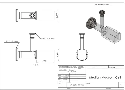
cell1_{with electronic feed through for the}_Rb_{alloy dispenser}2_{, Figure 2.3.}

~100

50.80

~210

1.33" CF Flange 2.75" CF Flange

50.80

DRAWN CHK'D APPV'D MFG Q.A

UNLESS OTHERWISE SPECIFIED: DIMENSIONS ARE IN MILLIMETERS TOLERANCES: Precision

+0.01, -0.01 mm

DEBUR AND BREAK SHARP EDGES

NAME SIGNATURE DATE

MATERIAL:

DO NOT SCALE DRAWING Quantity: 1

TITLE:

DWG NO.

SHEET 1 OF 1

A4

AR coated BK7 Glass

WEIGHT: Kyle Hardman

Nick Robins

Nick Robins Medium Vacuum Cell

[image:22.595.72.500.100.407.2]

Dispenser Mount

Figure 2.3: Machine drawing for the implemented medium vacuum cell. The position of the dispenser mount is noted.

In order to maintain the lowest pressure possible in the UHV chamber the MV and UHV cells are separated by an area of high impedance. This reduces convective heating effects on the atomic sample during the final stages of cooling. The impedance is achieved as shown in Figure 2.4 by separating the cells with a long stainless steel tube with a low conductance created by an aperture of 1 mm diameter 2 cm length. The aperture effectively reduces the unwanted gas flow from the MV to the UHV cells while allowing cooled atoms to be selectively ‘pushed’ between the cells. Section 3.1.3 discusses the selective transfer of atoms between the cells [53].

The UHV cell is a custom designed aluminum cell shown in Figure 2.53. The cell has 8 horizontal and 2 vertical 2.75” stainless steel (SS) conflat (CF) flanges as well as 8 hori-zontal 1.33” SS CF flanges. These flanges are used for cooling and trapping optical access and 2D MOT, vacuum pump, and long drop mounting. The chamber was designed to have magnetic coils wrapped directly onto the system thereby improving heat dissipa-tion and minimizing the distance between the coils and the atoms to optimize trapping. The orientation of the cooling and trapping beams in relation to the UHV cell is discussed in detail in Section 3.

An ∼2.6 m long drop region is mounted to the bottom of the UHV cell. This section allows for the free fall of atoms from the center of the UHV cell for up to 750 ms. The long drop region consists of 3 cells4_{allowing optical access connected via two} _∼_{1 m CF}

1_{Precision Glassblowing part# custom order} 2_{Alvatec alvasource part# AS-6-Rb-100-F} 3_{Atlas Technologies part# custom order}

(23)

Vacuum System 11

A A

2.75" CF Solid Copper Gasket

Mounting Nuts

1

20.40

7.62

127

SECTION A-A

UNLESS OTHERWISE SPECIFIED: DIMENSIONS ARE IN MILLIMETERS TOLERANCES: Standard

+0.1, -0.1 mm

NAME SIGNATURE DATE

MATERIAL:

DO NOT SCALE DRAWING Quantity: 1

TITLE:

DWG NO.

SHEET 1 OF 1

A4 Stainless Steel 316

Nick Robins

[image:23.595.100.527.83.387.2]

Nick Robins

Impedance

Figure 2.4: Machine drawing for the implemented high impedance line.

304.80 228.09 304.80

236.22 _12.70

31.75

304.80 38.61

10 x 2.75" SS CF Flange

8 x 1.33" SS CF Flange

UNLESS OTHERWISE SPECIFIED: DIMENSIONS ARE IN MILLIMETERS TOLERANCES: Precision

+0.01, -0.01 mm

NAME SIGNATURE DATE

MATERIAL:

DO NOT SCALE DRAWING _{Quantity: 1}

TITLE:

DWG NO.

SHEET 1 OF 1

A4 Aluminum

Nick Robins

Nick Robins Ultra-High Vacuum Cell

Long Drop Mount Pump Sysytem

[image:23.595.103.528.297.687.2]

Mount 2D MOTMount

(24)

nipples5_{. In conjunction with the UHV cell, the long drop allows four areas for imaging}

the atomic ensemble. The four imaging regions correspond to 0 → 25, 220, 530, and 750 ms of free fall.

The system responsible for pumping and maintaining vacuum in the apparatus is mounted to the UHV cell as shown in Figure 2.5. This systems consists of a passive Titanium-sublimation pump (Ti-sub)6and an active Ion pump (IP)7which provides the majority of the pumping.

2.5 Vacuum Performance

The assembled vacuum system placed under medium vacuum, 1×10−7Torr, and baked vertically in a fan forced oven at 160 C for 24 hours. Prior to cooling the apparatus the Ti-sub pump was fired 3 times to sufficiently coat the inner vacuum chamber with a Titanium film. This assists in the ‘freezing’ of gas to the walls during the cool down. Upon cooling to room temperature a pressure of 2×10−11Torr was reached, determined by the IP pressure gauge.

From this pressure reading, pipe conductance, and conservation of flow the pressure at any point along the system can be found [54]. Equations 2.6 and 2.7 give the conduc-tance of pipe (C) in the molecular flow regime and the pressure drop (∆P) required across a pipe in order the flow rate, whereTgasis the temperature of the background gas,mis the

mass of the gas,Dis the diameter of the pipe in cm,Lis the length of the pipe in cm, and Qis the gas flow rate in Torr-liters/second. For multiple pipes in series the conductance is additive.

C=3.81

Tgas

m

1/2

D3

L (2.6)

∆P= Q

C (2.7)

The flow rate of the system is found from the IP’s pumping speed at the achieved pres-sure. For the pump used here this gives ∼60 L/s at 2×10−11Torr (1.2×10−9Torr L/s) [55]. Figure 2.2 shows the pressure along the apparatus as 2×10−11, 2.2×10−11, 9.4× 10−11, 1.35×10−10, 2.27×10−10, 3.2×10−10, and 1×10−7Torr corresponding to the crit-ical regions of the IP, IP to UHV cell interface, center of the UHV cell, imaging region 2, imaging region 3, imaging region 4, and the MV cell. The pressure at various points in the apparatus is illustrated in Figure 2.2.

(25)

Chapter 3

87 _{Rubidium Cooling}

Cooling the atomic ensemble which constitutes the interferometer test mass is of the ut-most importance. A non-zero effective horizontal temperature (Te f f) leads to divergence

of the sample as it propagates through the interferometer. The divergence of the cloud has the potential to lead to a number of detrimental effects which may limit the interfer-ometer’s phase sensitivity.

The most pressing effect comes about from the cloud sampling various aberrations in the lattice beams during propagation [56]. A number of experiments have been car-ried out to investigate the affect wavefront distortions have on the interferometer phase sensitivity. These studies conclude that, even for clouds ofTe f f ≈ µK and beam diame-ters of<12 mm, this effect could be a large, although not limiting, source of phase noise [17, 57, 58].

A high divergence rate associated with a high sourceT_{e f f} leads to a drastic decrease in the test mass density during propogation ∼T2

e f fT3. This results in optically diffuse

clouds at the interferometer output ports requiring a more complicated imaging scheme in order to maintain adequate signal-to-noise (SNR). The phase noise associated with imaging SNR is discussed in Section 7.5.

The most obvious solution to such problems is to produce a test mass with the mini-mum amount of divergence possible. Typically, this is accomplished through a dual stage of laser cooling[59] consisting of a magneto-optical trap (MOT) [60] and polarization gra-dient cooling (PGC) [61, 62, 63]. Precision atom interferometers using the mentioned cooling methods obtainTe f f ranging from 1→3µK [14, 17, 64]. However, these temper-atures may not be low enough to overcome wavefront distortion effects. The temperature may be reduced further using more intricate laser cooling methods such as gray molasses [65, 66, 67] or Raman sideband cooling [68, 69, 70] but these will not be discussed here.

To further reduce the temperature, the atomic sample may be confined to a trap, gen-erally created via a magnetic quadrupole [71] or optical potential[72], where a sequence of evaporative cooling is subsequently implemented [73]. Using a combination of laser and evaporative cooling schemesTe f f 1 nK may be achieved [74]. Evaporative

tech-niques have been used to produces "point source" ultra-cold atomic ensembles for atom interferometry [35] further limiting the negative effects due to optical wavefront aber-rations. Although evaporative cooling is a powerful and effective method for reaching ultra-cold temperatures it is only possible through the loss of atom number.

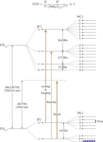
With the proper application of cooling techniques the required cloud temperature and density may be reached to achieve quantum state degeneracy thereby producing a Bose-Einstein condensate (BEC) [75, 76]. The theory for BEC formation and charac-teristics are covered in depth by many previous texts and will not be discussed in de-tail here [48, 77, 78]. Typically, BEC formation is realized when the ensemble’s

(26)

atomic spacing becomes less than the thermal de Broglie wavelength (λDB) thus

satisfy-ing the inequality in Equation 3.1, whereNis the number of atoms,Vis the ensemble’s volume, h is Planck’s constant, mis the atomic mass, kB is Boltzmann’s constant, and

λDB = h/(3mkBTe f f)1/2. The value of Equation 3.1 is generally referred to as

phase-space-density (PSD).

PSD= N V

h3 (3mkBTe f f)3/2

1 (3.1)

52_S 1/2 52_P

3/2

384.230 THz (780.241 nm)

3

2

1

0

-3 -2 -1 0 1 2 3

-2 -1 0 1 2 -1 0 1 0

-10 1 -2 -1 0 1 2

1 2

6.8 Ghz 72 MHz 157 Mhz 266 Mhz

282 THz (1064 nm)

Dipole Repump Cooling

& Imaging

m_fµ_Bg_jB |F’

|F

|m’f

[image:26.595.106.449.164.638.2]

|mf

Figure 3.1: The87Rb D2 transition structure including the Zeeman level splitting and orientation

important for magnetic trapping. Noted are the transitions used for cooling, imaging, repuming,

and optical trapping. At the completion of cooling the atoms occupy theF=1mf =−1 ground

state.

(27)

87_{Rubidium Cooling} ₁₅

driven it may still be characterized as an effective temperature of expansion providing an intuitive measure of kinetic energy 1₂mv2 ≈ 3₂kBTe f f.

In addition to the exceptionally low expansion rates of BEC sources, a number of other characteristics make them ideal propagators for atom interferometers, most notably a large spatial coherence encompassing the entire condensate. The advantages to this coherence are further discussed in Section 8.

The element used for the test mass in this apparatus is87Rb. An illustration of the

87_{Rb D}

2transition structure showing the relevant laser cooling, and trapping transitions

is given in Figure 3.1.

3.1 Laser Cooling

The behavior of a thermal collection of atoms (uncondensed) is well described by Boltz-mann statistics and as such has a well defined relation between the ensembles tempera-ture (T_{e f f}) and the root-mean-squared of velocity (vRMS) is given by the familiar Equation

3.2. Due to this relation methods for cooling thermal clouds focus on decreasingvRMS.

Laser cooling uses the transfer of photon momentum to atoms in order to decrease the sample’s velocity distribution in a deterministic manner.

3

2kBTe f f = 1 2mv

2

RMS (3.2)

3.1.1 Magneto-Optical Trap Theory

The standard laser cooling scheme, illustrated in Figure 3.2, is the magneto-optical trap (MOT). A hot atomic vapor is placed in a magnetic field produced by two coils in anti-Helmholtz configuration. This produces a magnetic field which is zero at the center and increases in magnitude with the radius. The exact form of the field and field gradient can be found and is discussed in Section 3.2.2. The magnetic field produces a position dependent Zeeman splitting for the atomic ensemble giving the ability to selectively in-teract with atoms at precise radii through proper tuning of the cooling light or varying the magnetic field gradient.

I

σ

+

σ

+

σ

+

σ

-σ

-z

x y

|mf

1

1 -10

0 -1

B

E

[image:27.595.108.301.551.746.2]

y’

Figure 3.2: Illustration of a typical

three-dimensional magneto-optical trap (3D MOT) for the laser cooling of atoms. The trap consists of 3 pairs of orthogonal circularly polarized beams intersecting at the zero field center of a mag-netic field created by two electromagnets in anti-Helmholtz configuration. The three beam pairs

are oriented along thex, y, and z axis,

respec-tively. Atoms are trapped at the magnetic field minimum as a result of the spatially dependent radiation pressure induced by the spatially

de-pendent Zeeman splittings of the atoms. (—)

(28)

The MOT cooling light may consist one, two or three pairs (one-dimensional MOT (1D), two-dimensional MOT (2D), or three-dimensional MOT (3D)) of counter propagat-ing narrow linewidth beams each with the ability to be frequency tuned near and to a cycling atomic transition, like that shown in Figure 3.1. By choosing that each pair of cooling beams is of orthogonal circular polarization (σ+andσ−), each beam is only res-onant with atoms occupying a single coordinate quadrant. Cooling and trapping in a 1D MOT is achieved in the following manner: Assume an atom occupies the+yquadrant and has velocity+v; when the atom passes the positiony0 the such thatm_fµBgjB=¯h∆ω

is satisfied the atom absorbs a photon from the beam; the atom spontaneously emits the absorbed photon randomly into 4π in the excited state lifetime; after a number of in-teractions (n) the momentum of the atom along they-axis has been altered bynphoton recoils and pushed toward the center; as the atom traverses pasty = 0 it becomes res-onant with the counter-propagating beam and is again pushed back towards the center; the frequency of light can be adjusted to address any spatial positiony; by sweeping the laser frequency and magnetic field gradient it is possible to highly compress the atom cloud.

Throughout the MOT process the initial absorbed photons provide cooling to the sam-ple whereas the spontaneously emitted photons heat. The mean square velocity of the sample is given by Equation 3.3 [79], whereΓis the linewidth of the transition, and∆ω is the detuning of the laser from the transition.

v2_RMS= ¯hΓ 4m

1+ (2∆ω

Γ )2

2|∆ω|

Γ

(3.3)

By minimizing Equation 3.3 and setting the kinetic energy equal to the 1Dthermal energy, similar to Equation 3.2, the minimum achievable temperature is found, Equation 3.4. The system is trivially extended to 3D. The minimum of Equation 3.4 is considered the Doppler temperature limit and is∼145µK for87Rbwith cooling beams on the F = 2 → F0 =3D2transition.

T_{e f f} = ¯hΓ 2kB

(3.4)

3.1.2 Polarization-Gradient-Cooling Theory

It is possible to laser cool below the Doppler limit using a polarization-gradient-cooling (PGC) scheme. The details of PGC have been exhaustively explored in previous work [63] and will not be discussed in detail here. Briefly, PGC arises from the spatially vary-ing polarization vector produced from the phase interference of the counter propagat-ing coolpropagat-ing beams. For the case of counter-propagatpropagat-ing orthogonal circularly polarized beams the electric field components as a function of distance are given by Equations 3.5 and 3.6, whereλis the frequency of light, andzis the propagation direction.

Ex=cos(

2π

λ z)−sin( 2π

λ z) (3.5)

Ey=sin(

2π

λ z)−cos( 2π

λ z) (3.6)

(29)

87_{Rubidium Cooling} ₁₇

End

σ+

σ

-0 λ 2λ 3λ 4λ 5λ 6λ 7λ 8λ 9λ 10λ

z Position (m) Ey

(ar

b.)

0

-1 1

0 -1

1

Ex(arb.)

Ey

(ar

b.)

0

-1 1 Side

z

Figure 3.3: The spatially

depen-dent polarization orientation formed through the counter-propagation of right (σ+) and left (σ−) handed circu-larly polarized light. A helical struc-ture is seen, created by linear polar-ization which rotates about the

prop-agation axis undergoing a 2π

rota-tion over the wavelength of light (λ). The total electric field remains con-stant over all space showing the ex-pected lack of intensity interference.

spatially rotating linear polarization. The polarization rotates through 2π in a length scale determined byλ. As would be expected, the magnitude of the electric field vector remains constant for all spatial positions resulting in no intensity variations along the beams.

In order for PGC to work effectively the quantization axis of the atoms must be well defined by the polarization axis of the light and therefore the background magnetic field should be minimized. The cooling mechanism is best described starting with an individ-ual atom at rest at positionz0. The atom exists in a linearly polarized (π) light field with quantization axis defined by the field. The atom has a probability distribution among it’s|mfiground states which can be found directly from the Clebsh-Gordon coefficients

pertaining to the cooling transition.

If the atom is now given a velocity (v) it begins sampling the rotating polarization field. The cooling mechanism is induced from a non-adiabatic following of the ground state populations as the atom propagates through the varying quantization axes. The non-adiabatic following produces an imbalance in the ground state populations leading to optical pumping from the cooling beams. This manifests itself as an imbalance in radiation pressure between the counter-propagating beams which provides a force in the opposite direction tov.

In the limit of∆ω Γthe equilibrium temperature for counter-propagating circu-larly polarized cooling beams in given in Equation 3.7 [63], whereΩis the Rabi frequency of the cooling transition as defined in Section 4.1. In practice Te f f is limited by the

absorption of spontaneously emitted photons limiting the temperature to the photon re-coil limit, Equation 3.8, wherek=2π/λ. The recoil limit for the87Rb F=2→F0 =3D2

cooling transition is∼150 nK.

Te f f =

29 300

¯ hΩ2 kB|∆ω|

(3.7)

Trecoil=

¯ h2k2 3mkB

(3.8)

3.1.3 Laser Cooling System

(30)

implementation of cooling on a pure cycling transition with no loss of atoms to other states. Although theF=2→ F0 =3 transitions used here is a cycling transition the close proximity of theF =2→F0 =2 (∆ω=2π×266 MHz) line gives rise to significant atom loss to theF=1 ground state through off resonant transitions. As a consequence, a beam resonant with theF=1→F0 =2 transition is required to repump the lost atoms back to the cooling line. The rate of off resonant pumping to theF=1 ground state is discussed in Section 5.1.1. Figure 3.1 shows the87Rb D2structure.

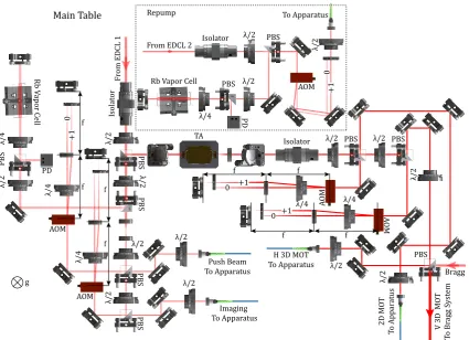
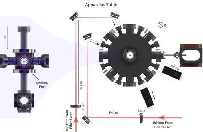
[image:30.595.74.500.344.652.2]

In order to efficiently cool, a standard technique is to separate the cooling into two vacuum regions: one low vacuum region where the atoms are produced and precooled in a 2D MOT; and a second ultra-high vacuum (UHV) chamber where a 3D MOT is im-plemented. The addition of the low vacuum region requires a separate ‘push’ beam to transfer atoms through a high impedance line to the UHV chamber. The details of the vacuum system are discussed in Section 2. Due to the sensitivity of the Bose-Einstein condensate to stray resonant light the optics are split between two tables: The main ta-ble, Figure 3.4, is completely sealed with high neutral density acrylic to minimize light leakage and encompasses all the optics necessary for the amplification, switching and frequency manipulation of the light; and the second table corresponds to the apparatus table, Figure 3.6, where the light is directed into the science cell.

λ/4 Isolat or PBS λ/2 PBS λ/2 TA Rb Vapor Ce ll PBS λ/2 PD _λ/2 λ/2 AOM AOM λ/4 λ/4

Isolator λ/2 PBS λ/2 PBS

λ/2 PBS λ/2 λ/2 λ/4 λ/4 f f f f f f _f f AO M AO M PBS PBS λ/2 λ/2 g

Main Table Repump

Push Beam To Apparatus

Imaging

To Apparatus _2D MO

T

To

Appar

at

us

H 3D MOT To Apparatus To Apparatus V 3D MO T To Br agg S yst em Bragg

From EDCL 2

Fr

om

EDCL

1 Isolator λ/2 PBS

λ/2

Rb Vapor Cell

λ/4 PD

PBS λ/2 _AOM

+1 0 +1 0 0 +1 +1 0

Figure 3.4: Illustration of the optics system responsible for the production of the 2D and 3D MOT, imaging, push, and repump beams corresponding to the main optics table only. The external cav-ity diode lasers are not shown. Abbreviations are as follows: external cavcav-ity diode laser (ECDL);

half-wave plate (λ/2); quarter wave plate (λ/4); polarizing beam splitter (PBS); acoustic-optic

(31)

87_{Rubidium Cooling} ₁₉

The optics corresponding to the 2D MOT, 3D MOT, imaging and push beam are all seeded on the main table from a single external cavity diode laser (ECDL)1 producing ∼40 mW of linearly polarized light . The output of the ECDL initially passes through a number of optical isolators2producing 160 dB isolation which limits the back transmitted light from a tapered amplifier (TA) further down the optics line. The high degree of isolation for ECDL 1 is paramount as any reverse transmitted light from the TA will inhibit the ECDL from running single mode. On the output of the isolators the light is split via a half-waveplate (λ/2) and polarizing beam splitter (PBS) along two paths. The transmitted light is further split along three paths used for the push beam switching and frequency control, the imaging switching and frequency control, and the absolute frequency locking scheme for the ECDL. The reflected light is used for the 2D and 3D MOT cooling beams.

The switching and frequency control lines for the imaging and push beams are of identical design originating from individual PBSs and propagating as follows: light is passed through an acoustic-optic modulator (AOM)3such that the first order diffraction mode (+1) is dominant; all light then passes through a quarter-wave plate (λ/4) and a lens; following the lens an iris blocks the zeroth order diffraction before the light is retroreflected along the same path; after the second pass through theλ/4 the light has the opposite linear polarization so it will pass the PBS; with proper alignment the first order diffraction on the second AOM pass will be along the same vector as the input beam; the frequency shifted light is then coupled to the apparatus table through a polarization maintaining optical fiber4[80]. Placing the lens such that both the AOM and retroreflector are at the focal length will ensure proper overlap and mode matching on the incoming and reflected beam.

In order to reduce unwanted birefringent effects in the fiber such as polarization rota-tion or mixing, the incident beams are aligned to the fast and slow polarizarota-tion axes of the fiber using aλ/2. Proper axis alignment will result in an extinction ratio of∼23 dB while the fiber is mechanically or thermally stressed. The light on the output of the double pass AOM will have been frequency shifted by twice the AOM driving frequency resulting in beams with frequencies 2ω1and 2ω2, whereω1andω2are the driving frequencies of the

AOMs.

All AOMs in the cooling system are driven through a voltage controlled oscillator (VCO)5in series with a transistor-transistor logic switch (TTL)6and radio frequency am-plifier7. The voltage control and switch signal for the VCO and TTL is provided from the control computer.

The absolute frequency reference and locking scheme for the ECDL is produced from the standard saturated absorption spectroscopy (SatAbs) of a Zeeman modulatedRb va-por cell. The detailed discussion of SatAbs is provided in Reference [81]. The SatAbs optics are relatively simple and consist of an initially linearly polarized beam passing through a PBS andλ/4 creating circularly polarized light. The light then passes through a Zeeman modulatedRbvapor cell and is retroreflected back along the same path. At the second pass of theλ/4 and PBS the light is reflected and incident on a photodiode (PD)8.

1_{MOGLabs Littrow extended cavity diode laser part# ECD004} 2_{Thorlabs optical isolator part# IO-5-780-HP}

3_{AA Opto-electronics modulator part# MT110-A1-IR}

4_Schäfter₊_{Kirchoff patch cable part# PMC-780-5.3-NA012-3-APC-500-P} 5_{Mini-Circuits oscillator part# ZX95-100-S+}

6_{Mini-Circuits high isolation switch part# ZASWA-2-50DR+} 7_{Mini-Circuits amplifier part# ZHL-3A-S+}

(32)

Figure 3.5: The saturated

absorption spectrum of Rb

centered around the 87_Rb

D2 transition. All

spec-tral features labeled as x-y denotes a crossover

transi-tion, i.e. the feature F =

2 → F0 = 2−3

corre-sponds to a frequency

mid-way between theF = 2 →

F0 = 2 and the F = 2 →

F0 =3 lines. The crossover

transitions are a result of the matching Doppler con-ditions of atoms moving in opposite directions[82]. 0.0 -0.1 -0.2 -0.3 -0.4 -0.5 -0.6 -0.7 -0.8 -0.9 -1.0 7 6 5 4 3 2 1 0 0.0 0.1 0.2 0.3 0.4 0.5 400 200 0 -200

-400 -200 -100 0 100 200

Detuning (GHz) Tr ansmission (ar b) Tr ansmission (ar b)

87_{Rb D2} 85_Rb 85_Rb 87_{Rb D2}

F=2 F’=3 F=1 F’=2

0.0 0.1 0.2 0.3 0.4 0.5 Tr ansmission (ar b) F=2 F’=? 3 2-3 1-3 2 1-2 1 Detuning (MHz) F=1 F’=? Detuning (MHz) 2 1-2 0-2 1 0-1 0

If the frequency of the input light is scanned a saturated absorption spectrum such as that in Figure 3.5 is seen. The absolute energy and energy difference for all relevant87Rb transitions can be found in Figures 3.5 and 3.1. The signal from the PD which contains theRbSatAbs is passed into a locking loop9which has active current and grating control of the ECDL.

The light used for the 2D and 3D MOT beams is steered and focused into a TA10 pro-ducing up to 2 W at the output. After passing through an optical isolator, two sets ofλ/2 and PBSs split the light into the separate switching and frequency control setups corre-sponding to the 2D and 3D MOT. The 2D and 3D MOT frequency control is accomplished through standard double pass AOM setups as described above for the imaging and push beam lines. Upon exiting the frequency control setups the 2D MOT line is steered directly into a fiber, coupling the light to the apparatus table.

The orientation of the magnetic coils responsible for generating the MOT and mag-netic quadrupole trap requires that one pair of MOT beams be aligned to vertical, along the same path as the Bragg beams. To facilitate this the 3D MOT beam is split once again with the first path (V 3D MOT), at 1/3 the total power, being sent to the Bragg system. Once in the Bragg system the V 3D MOT light is coupled with the Bragg light and then coupled to the apparatus table. The second path (H 3D MOT), at 2/3 total power, is di-rectly fiber coupled to the apparatus. As explained above, the proper alignment of the light polarization axis to the fast or slow axis of the optical fibers is essential.

A separate ECDL is responsible for all repump light due to the 6.8 GHz splitting be-tween theF=2→F0 =3 andF=1→F0 =2 transitions. The ECDL produces∼40 mW of linearly polarized light which is passed directly through an optical isolator. On the output of the isolator the light is split between two paths via a λ/2 and PBS. The first path is steered to a standard SatAbs setup identical to that discussed above. The sec-ond path is passed through an AOM such that the+1 mode is dominant. Prior to fiber

(33)

87_{Rubidium Cooling} ₂₁

B λ/4

λ/4

PBS

Isolated Mirror

λ/2

PBS

λ/4

g g

Apparatus Table

H

3D

MO

T

2D

MO

T

Repump

Push

V

3D

MO

T

Figure 3.6: Illustration of the optics system responsible for the production of the 2D and 3D MOT, push, and repump beams corresponding to the apparatus table only. The inset shows the vertical

orientation of the vertical magneto-optical trap beam. (—) Induced magnetic field for the

three-dimensional magneto-optical trap. Abbreviations are as follows: half-wave plate (λ/2); quarter

wave plate (λ/4); polarizing beam splitter (PBS); horizontal components of the three-dimensional

magneto-optical trap (H 3D MOT); vertical component of the three-dimensional magneto-optical trap (V 3D MOT); and component of the two-dimensional magneto-optical trap (2D MOT).

coupling the+1 mode to the apparatus, the zero order mode is dumped onto a iris. Once coupled to the apparatus table the light is distributed as illustrated in Figure 3.6. All beams are outcoupled with large aperture fiber collimators11 giving beam waists of 2 cm FWHM. The 20 mW of repump light passes through aλ/2 and two PBSs. A fraction of the light is reflected from the first PBS and overlapped with the 2D MOT light. The remaining repump light is passed through the second PBS and overlapped with the 3D MOT light. The 2D and 3D MOTs may be partially optimized by adjusting the fraction of repump which is shunted to each line.

The 180 mW 2D MOT line’s polarization is rotated such that it passes its initial PBS and is phase delayed such that the light is of circular polarization. Before entering the low vacuum cell the beam is expanded to 5 cm FWHM. The 2D MOT in formed from a single recycled beam which passes horizontally through the cell, is reflected using three mirrors to then propagate through the cell vertically, passes through anλ/4, and is retro reflected along the original path now having orthogonal polarization.

The 85 mW H 3D MOT beam is totally reflected and overlapped with the repump beam on a PBS at the outcoupler. Aλ/2 and PBS then splits the light equally along two paths which make up the horizontal 3D MOT lines. Each line is passed through aλ/4 making it circularly polarized prior to entry into the science cell. On the opposing side of the cell the beams are passed through a secondλ/4 and retro reflected.

(34)

The 30 mW V MOT beam is outcoupled to the apparatus table using the same ver-tically oriented large aperture outcoupler as the Bragg beams and follows the same se-quence of optical elements as the H 3D MOT beams with the addition of a PBS before of the retroreflector.

At the apparatus table the push beam is out coupled and polarization cleaned with a PBS. The beam is made to have circular polarization and is aligned overlapping with the atom fluorescence from the 2D MOT such that its vector is through the center of the impedance line.

3.1.4 Laser Cooling Procedure and Performance

HotRbatoms are continuously created in the low vacuum cell by passing current through a metallic dispenser which contains aRballoy12. This produces a backgroundRbvapor of 10−7Torr. The 2D MOT, push, repump, and 3D MOT light are turned on simultane-ously. Figure 3.7 is a graphical representation of the laser cooling procedure showing laser detunings from the relative transitions shown in Figure 3.1, amplitudes, magnetic field gradients, and Te f f. Radiation pressure from the 12 MHz red detuned (−12 MHz)

2D MOT light cools the hot vapor into a long cigar shaped cloud which is colinear with the high impedance line. The push beam, which is 17 MHz blue detuned (17 MHz), pro-vides a directional group momentum to the cooled cloud such that they are continuously pushed from the low vacuum cell and into the UHV cell. Once in the UHV cell the 2D cooled atoms are trapped in the 3D MOT formed using−23 MHz detuned MOT light, resonant repump light, and a magnetic field gradient of 26 G/cm. The 3D MOT is al-lowed to load for 5.99 s after which the 2D MOT and push light are extinguished. In a typical 6 s loading procedure 5×109_{atoms are collected in the 3D MOT with a}

temper-ature of 120µK. This number can be increased to 1×1010 atoms in 10 s with the same temperature.

After 5.99 s the push and 2D MOT light are extinguished. It is essential that the back-ground magnetic field bias now be zero. The PGC procedure is started with the repump detuning, 3D MOT light detuning, and magnetic field gradient jumped to−9 MHz,−40 MHz, and 7.5 G/cm, respectively. This cools and compresses the original cloud. The system re-mains at the stated values for 27 ms as cooling continues. Over the final 20 ms of laser cooling the repump detuning, 3D MOT light detuning, and magnetic field gradient are slowly ramped to −10 MHz, −54 MHz, and 0 G/cm, respectively. The 3D MOT ampli-tude is also ramped down during this time and finally switched to zero at 6.04 s. At the final stage of PGC, ∆Bz = 0, the cloud has reached a temperature of 20µK. As the de-tuning of all beams increases and the power of the 3DMOT light decreases the radiation pressure is no longer able to support the atoms in the gravitational field. At this point the cloud is trapped in a hybrid magnetic and optical cross-dipole trap [83] for further cooling, as outlined in Section 3.2.

(35)

87_{Rubidium Cooling} ₂₃

-12

17 Push

2D MOT

-10 -7.5 -5.0 -2.50.0

-45 -35 -25

20 10 0

6.04 6.02

6.00 5.98

0 5.0

4.0

3.0

Δω

(MHz)

Δω

(MHz)

Δω

(MHz)

Amp.

(ar

b.)

∇B

z

(G/cm)

Time (s) Repump

3D MOT

Coils

120

µK

20

µK

Figure 3.7: Illustration of the push, 2D magneto-optical trap (MOT), re-pump, and 3D MOT light detuning, 3D MOT light amplitude, and MOT magnetic field gradient as a function of time after run start. The laser cool-ing is divided into two regions: the

first from 0 → 5.99 s corresponds

to the initial MOT which achieves a

temperature of 120µK; and the

sec-ond from 5.99 → 6.04 s corresponds

to polarization gradient culling and reaches a minimum temperature of 20µK.

3.2 Evaporative Cooling

Evaporative cooling of atomic samples relies on the selective removal of hot atoms al-lowing the remaining atoms to rethermalize to a lower temperature. There are a number of techniques which allow for evaporative cooling to occur, all of which involve trapping atoms in a harmonic potential. Details relating to the confinement of atoms in a magnetic and optical trap will be discussed here.

3.2.1 Evaporative Cooling Theory

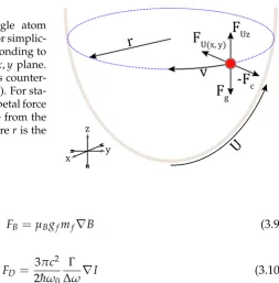
The confinement of an atomic sample to a potential naturally induces a spatial depen-dency to the spread in the atomic velocities. This can easily be shown when considering the somewhat simplified system shown in Figure 3.8 where the atomic motion correlated to temperature is confined to thex,yplane.

An atom placed in a potential (U) will feel a force (F_U(x,y)) which for magnetic and

electro-magnetic fields is proportional to the field gradient (∇). Equations 3.9 and 3.10 give the applied force for a neutral atom in a magnetic or optical potential, whereµB is

the Bohr magneton,gf is the Landé g-factor,mf is the magnetic spin state,cis the speed

of light,ω0is the frequency of the nearest atomic resonance, and Iis the optical intensity.

For a typical harmonic potential this gradient increases with the radius (r), whereas a quadrupole potential has a constant field gradient. In order to obtain a stable orbit in the potential the centripetal force (Fc = mv2/r =3kBTe f f/r) andFU(x,y)must be equal. This

gives a general mapping ofvtorand as a consequencertoTe f f, where the stable orbital