A geomorphology based reconstruction of ice volume distribution at
the Last Glacial Maximum across the Southern Alps of New Zealand
William H.M. James
a,*, Jonathan L. Carrivick
b, Duncan J. Quincey
b, Neil F. Glasser
c aSchool of Geography and Leeds Institute for Data Analytics, University of Leeds, Leeds, West Yorkshire, LS2 9JT, UKbSchool of Geography and water@leeds, University of Leeds, Leeds, West Yorkshire, LS2 9JT, UK cDepartment of Geography and Earth Sciences, Aberystwyth University, Wales, SY23 3DB, UK
a r t i c l e i n f o
Article history:
Received 11 February 2019 Received in revised form 26 June 2019
Accepted 28 June 2019
Keywords:
Geomorphology Glacial Glaciation Glaciology Quaternary Southern pacific
a b s t r a c t
We present a 3D reconstruction of ice thickness distribution across the New Zealand Southern Alps at the Last Glacial Maximum (LGM, c. 30e18 ka). To achieve this, we used a perfect plasticity model which could easily be applied to other regions, hereafter termed REVOLTA (Reconstruction of Volume and Topography Automation). REVOLTA is driven by a Digital Elevation Model (DEM), which was modified to best represent LGM bed topography. Specifically, we removed contemporary ice, integrated offshore bathymetry and removed contemporary lakes. A review of valley in-fill sediments, uplift and denudation was also undertaken. Down-valley ice extents were constrained to an updated geo-database of LGM ice limits, whilst the model was tuned to best-fit known vertical limits from geomorphological and geochronological dating studies. We estimate a total LGM ice volume of 6,800 km3, characterised pre-dominantly by valley style glaciation but with an ice cap across Fiordland. With a contemporary ice volume of approximately 50 km3, this represents a loss of 99.25% since the LGM. Using the newly created ice surface, equilibrium line altitudes (ELAs) for each glacier were reconstructed, revealing an average ELA depression of approximately 950 m from present. Analysis of the spatial variation of glacier-specific ELAs and their depression relative to today shows that whilst an east-west ELA gradient existed during the LGM it was less pronounced than at present. The reduced ELA gradient is attributed to an overall weakening of westerlies, a conclusion consistent with those derived from the latest independent climate models.
©2019 The Authors. Published by Elsevier Ltd. This is an open access article under the CC BY license (http://creativecommons.org/licenses/by/4.0/).
1. Introduction
The New Zealand Southern Alps is a key site for glacial recon-struction studies and is one of only three mid-latitude southern hemisphere locations at which extensive Pleistocene glaciation occurred. Furthermore, the geomorphological record of the Last Glacial Maximum (LGM) in New Zealand has excellent spatial and
temporal coverage (Barrell et al., 2011) and has long been
recog-nized for its potential for improving understanding of former
cli-matic conditions via glacier geometry reconstruction (e.g.Porter,
1975b). LGM ice thickness has previously been reconstructed for
individual catchments in New Zealand (e.g.Putnam et al., 2013) and
at the regional scale (Golledge et al., 2012), although uncertainty
still exists regarding the extent, timing and associated climatic
conditions.
Glacial reconstruction in New Zealand presents significant
challenges as the extreme relief and high precipitation of parts of the Southern Alps gives rise to a complex yet large-scale system (Chinn et al., 2014). To date, the work byGolledge et al. (2012)is the only attempt at a regional reconstruction of LGM ice thickness, and that was achieved using the Parallel Ice Sheet Model (PISM). They used a Digital Elevation Model (DEM) and climate parameter inputs
(spatially uniform scaling of contemporary conditions) to bestfit
the areal ice limits delimited byBarrell (2011)(Fig. 1). Some
rela-tively large (tens of kilometers) discrepancies must be noted however, where the PISM was unable to recreate known
down-valley limits derived fromfield-based observations and
indepen-dently dated landforms. Specifically, in comparison to the mapping
ofBarrell (2011),Golledge et al. (2012)underestimated ice extent in
the eastern outlets including the Rakaia and Waimakariri (Fig. 1).
As an alternative to top-down climate models, a number of
bottom-up,‘topography based’techniques have been developed for
*Corresponding author.
E-mail address:w.h.m.james@leeds.ac.uk(W.H.M. James).
Contents lists available atScienceDirect
Quaternary Science Reviews
j o u r n a l h o m e p a g e : w w w . e l s e v i e r. c o m / lo c a t e / q u a s c i r e v
https://doi.org/10.1016/j.quascirev.2019.06.035
estimating contemporary ice thickness (Linsbauer et al., 2012; James and Carrivick, 2016) and palaeo-ice thickness (Pellitero et al.,
2016). With the Southern Alps presenting excellent input datasets
for LGM ice thickness reconstruction in this manner (high resolu-tion DEMs and well constrained down-valley ice limits), and with climate driven models currently unable to resolve known ice limits
in some catchments (i.e.Golledge et al., 2012), we developed and
applied a topography driven model to produce a new estimate of distributed LGM ice thickness. Our approach is similar to that
described byPellitero et al. (2016)and in effect a reverse of the
VOLTA contemporary ice thickness model developed byJames and
[image:2.595.100.505.60.620.2]Carrivick (2016). As such the model is hereafter referred to as REVOLTA (Reconstruction of Volume and Topography Automation). Using this approach, the aim of this study is to reconstruct the Fig. 1.Location map of regions referred to in this study and previous delineations of LGM ice extent. Note the mismatch between extents estimated byBarrell (2011)andGolledge
LGM distributed ice thickness across the Southern Alps of New Zealand to help improve our knowledge of glaciological and asso-ciated climatic conditions during the LGM in the Southern Hemi-sphere. Being far from the centres of Northern Hemisphere glaciation, research in New Zealand provides the potential to examine the climatic effects of changes in Northern Hemisphere ice sheets on Southern Hemisphere climate, as well as events of origin
in the Southern Hemisphere (Shulmeister et al., 2019).
2. Methods: a framework for reconstructing distributed ice thickness
REVOLTA initially calculates the surface profiles of former
gla-ciers along a network of centrelines using an exact solution of a
‘perfect plasticity’ approach. Ice thickness values are iteratively
calculated along each centreline, starting at the former terminus
position. A‘nearest neighbour’routine is used in conjunction with
the DEM to convert the centreline thickness points into a 3D distributed thickness. REVOLTA expands on the 2D only model
presented byBenn and Hulton (2010)and is similar in nature to
Pellitero et al. (2016). A schematic diagram of the REVOLTA
framework is shown in Fig. 2 and major processing steps are
described in the following sections.
2.1. Constructing a DEM to represent the LGM
A digital elevation model (DEM) forms the primary input of REVOLTA. Whilst contemporary DEMs are often used to represent
former glacier beds (Trommelen and Ross, 2010), the most accurate
results will be achieved if the DEM is representative of the period of reconstruction (i.e. the LGM). To achieve this, we used a
contem-porary 8m resolution DEM (Geographix, 2012), to which we applied
a number of corrections: (i) removing contemporary ice thickness, (ii) integrating offshore bathymetry, (iii) removing modern-day
lakes thatfill the remnants of troughs evacuated by LGM ice. The
impact of uplift, denudation and postglacial sediment valley infill
was also considered.
2.1.1. Removal of contemporary ice from the DEM
The Southern Alps currently supports around 3,000 glaciers
covering an area of approximately 1,200 km2 (Chinn, 2001).
Contemporary ice was removed from the DEM to estimate a surface which better represents LGM bed conditions. This removal was achieved using the distributed ice thickness results of the VOLTA
model (James and Carrivick, 2016) to compute modern day ice
thickness (e.g. as for Southern South America byCarrivick et al.
(2016)and as for the entire Antarctic Peninsula byCarrivick et al. (2019)). VOLTA was run on all contemporary glaciers>1 km2and
resulted in a total (contemporary) ice volume of 40.68 km3with a
maximum thickness of over 550 m. Full details of the VOLTA model
can be found inJames and Carrivick (2016), whilst details of the
contemporary ice thickness distribution of the Southern Alps can
be found inJames (2016).
2.1.2. Appending an offshore DEM
Sea level during the LGM was approximately 125 m below
cur-rent levels (Milne et al., 2005), with palaeoglaciers on the West
Coast of New Zealand inferred to extend into these currently
sub-marine environments. Specifically, analysis of areal LGM limits
delineated byBarrell et al. (2011)revealed that 2.5% of a total LGM
glaciated area occurred beyond the present coastline and conse-quently outside the limits of the standard DEM. Therefore, an alternative topographical source was required for these presently-offshore areas. For this purpose, we used the National Institute of Water and Atmospheric Research (NIWA) 250 m resolution
bathymetric dataset (Mitchell et al., 2012) and these data were
appended to the existing DEM. To create a seamless dataset, the bathymetry was resampled to the resolution of the land surface (8 m) and merged.
2.1.3. Contemporary lakes
Whilst palaeoglaciers extended past the contemporary coast-line, they also occupied areas where contemporary lakes now exist, for which standard DEMs represent the water surface level and not the underlying bathymetry, thus obscuring the former glacier bed topography. Substantial lakes inboard of LGM moraine sequences of
the Southern Alps are over 450 m deep (e.g.Irwin, 1980),
high-lighting the importance of considering their bathymetry. Many of these lakes developed at the end of the LGM and were in contact
with a calving ice margin (Sutherland et al., 2019).
To produce a DEM more representative of LGM conditions, the water depth of major lakes within the model domain was sub-tracted from the initial DEM. Each map was georeferenced, with water depth contours ranging in interval between 5 m and 100 m digitized. Bathymetry was adjusted to the lake level of the DEM before a gridded surface was interpolated using the hydrologically
correct ANUDEM algorithm (Hutchinson, 1989). These data were
subsequently merged with the DEM, helping to produce a surface more representative of LGM bed conditions.
Whilst sediment deposition has occurred in these lakes since
the LGM, there is insufficient data to remove this from the DEM. Of
the limited data which does exist, cores from Lake Ohau found sediment thicknesses (deposited since lake formation at the end of the LGM) of 82 m and 43 m beneath 101 m and 68 m of water
respectively (Levy et al., 2018). This shows that whilst the presence
of such sediment needs to be acknowledged, water depth alone accounts for the majority of the difference between the LGM bed and the contemporary DEM surface. By removing the water depth, our study accounts for over 60% of the difference between the LGM bed and the contemporary DEM, something which has not been
considered by previous studies (e.g.Golledge et al., 2012).
2.1.4. Uplift and denudation
Uplift and denudation are processes that modify the landscape,
meaning their influence on the DEM needs to be considered. Whilst
these changes are commonly too small to introduce significant
error (Finlayson, 2013) and are thus commonly not included in ice
thickness modelling studies (Golledge et al., 2012;McKinnon et al.,
2012), here we assess how robust their omission is in terms of
impacting ice volume of the Southern Alps.
Post-LGM isostatic rebound in New Zealand is considered to
have been minimal (Pickrill et al., 1992), with Mathews (1967)
suggesting a maximum of 30 m rebound. However, tectonic uplift
rates in the Southern Alps are high, with the Pacific plate being
compressed into the Australian plate (Coates, 2002). Whilst long
term Cenozoic uplift rates of 0.1e0.3 mm yr1were estimated by
fission track thermochronology (Tippett and Kamp, 1995), rates
during the Pleistocene and Holocene are thought to have been
greater (Adams, 1980). The Paringa River site (location shown in
Fig. 1) provides one of the few robust constraints, with Pleistocene
to Holocene rates calculated at 8±1 mm yr1(Norris and Cooper,
2001). However, this rate is not thought to be representative of
the Southern Alps as a whole as the uplift pattern was highly
spatially variable, as evidenced by tilted lake shorelines (Adams,
1980).
Since AD 2000, GPS measurements have been collected along a transect running broadly perpendicular to the Alpine Fault, providing further information on the distribution of uplift rates across the Southern Alps. Results show a maximum average vertical
and critically, rates reduce rapidly with distance from the Alpine Fault, with measurements 29 km from the fault recording an uplift
rate of just 1.8±1 mm yr1, whilst no significant vertical rise was
measured at 68 km (Beavan et al., 2007). As these GPS
measure-ments record current rates, it is acknowledged that they are not necessarily applicable to longer (glacial) timescales. Nonetheless, with contemporary uplift rates reducing exponentially with
dis-tance from the Alpine Fault and no significant rise recorded at
68 km from the fault, and in lieu of any other geological data per-taining to long-term and spatially-distributed uplift rates, it is likely that much of the model domain for an LGM ice reconstruction would fall within relatively low uplift areas. This interpretation is
consistent with the inferred uplift pattern ofAdams (1980), with
the majority of the LGM ice extent occupying low uplift regions. Importantly, denudation effectively counteracts uplift, with long
term rates in the Southern Alps approximately equal (Adams, 1980).
For example, whilst the highest peak in the Southern Alps (Aoraki,
Mount Cook) is 3,724 m high, the total amount of uplift during
orogeny is estimated to be approximately 15e20 km (Kamp et al.,
1989).Tippett and Kamp (1995)provide one of the few quantifi
-cations of denudation, using fission track thermochronology to
estimate long term Cenozoic denudation rates ranging from
~2.5e0.5 mm yr1, decreasing with distance from the Alpine Fault.
This is supplemented by contemporary river load measurements by Adams (1980)who estimated the total river load of the Southern
Alps to be 700±200109kg yr1whilst basin averaged rates for
the Nelson/Tasman region are estimated to be between 112 and
298 t km2yr1(Burdis, 2014). Whilst providing a useful insight
into denudation rates, these estimates are not sufficient to
construct a regional distribution required for DEM modification.
In summary, whilst it is acknowledged that uplift and
denuda-tion have modified the geomorphological expression of the
[image:4.595.102.501.64.526.2]contemporary DEM. Furthermore, with rates of both uplift and denudation decreasing with distance from the Alpine Fault, much of our model domain falls within relatively low uplift/denudation areas. With the New Zealand land mass largely in its present
configuration by the mid-Pleistocene (Barrell, 2011), we therefore
made no further modifications to the DEM. These issues of tectonic
deformation and denudation will become increasingly prevalent for older glaciations, so care must be taken if seeking to reconstruct earlier glacial episodes.
2.1.5. Postglacial sediment valley infill
Large volumes of sediment accumulated in valley floors is a
commonly noted feature of the Southern Alps (McKinnon et al.,
2012). This process of landscape modification has previously been
recognized as a potential source of uncertainty when
reconstruct-ing palaeoglaciers in New Zealand (Golledge et al., 2012) and needs
to be considered when using a DEM to represent a former glacier beds.
It was initially postulated that the majority, or entirety of valley
fill in the New Zealand Southern Alps was deposited post-LGM
(Suggate, 1965; Adams, 1980) simply due to the‘absence of any
conflicting evidence’Adams (1980, p. 77), with some contemporary
research supporting the hypothesis that glaciers did indeed erode
to bedrock at the LGM (Thomas, 2018). However, this notion has
been challenged for the down valley reaches of LGM glaciers in the
Southern Alps, with Rother et al. (2010) suggesting that recent
glaciations in the Hope Valley (see Fig. 1for location) were not
powerful enough to cause extensive erosion and overrode pre-LGM sediments rather than removing them. At this location, infrared stimulated luminescence (IRSL) dating and sediment analysis found the majority of material was deposited during the pre-LGM period of 95.7 to 32.1 ka with only approximately 30 m of sediment accumulation occurring post LGM, overriding 200 m of previous
deposits (Rother et al., 2010). This pattern is consistent with seismic
investigation in the Franz Josef Valley byAlexander et al. (2014),
suggesting that the LGM bed was well above the bedrock. A
modelling study by McKinnon et al. (2012) also supports the
concept of LGM glaciers overriding pre-existing sediment, using a variety of models to simulate the LGM bed of the Pukaki glacier. The notion of pre-LGM sediment surviving in glaciated valleys is also consistent with studies outside of New Zealand, with pre LGM deposits found beneath more recent sediments in the European
Alps (e.g.Hinderer, 2001).
In summary, recent field based observations and modelling
studies provide evidence that LGM glaciers often overrode pre-existing sediments to some extent and did not always reach bedrock. Whilst it may seem surprising that gravels were able to
survive the entirety of the LGM,Shulmeister et al. (2019)suggests
that rapid water drainage through these stratified gravels resulted
in motion being initially limited to the slow and inefficient process
of internal ice deformation, allowing ice advance without sub-stantial erosion of the underlying substrate. As such, whilst
tech-niques exist to estimate and remove the entirety of sediment infill
from a DEM (e.g.Harbor and Wheeler, 1992;Jaboyedoff and Derron,
2005), this approach is not deemed appropriate for the regional
scale modelling of LGM glaciers in the New Zealand Southern Alps. With some sediment surviving, LGM bed elevations lie some-where between the contemporary DEM and the level that would
exist if all postglacial valley-fill were removed. However, since
inferred LGM sediment thickness is only available for a few select
locations (e.g.McKinnon et al., 2012), there are not enough data to
generate a regional distribution of the LGM bed surface beneath
Holocene valleyfill sediments. Therefore, with the consensus in the
literature suggesting that at least some sediment was present pre-LGM, for the regional scale modelling, REVOLTA was applied
without removing post LGM sediment.
2.1.5.1. Distributed post-LGM sediment thickness of the Pukaki Valley.
As discussed in section2.1.5, regional modelling was performed
without removal of any post-LGM sediment as there is insufficient
data to generate a regional distribution. However, modelling by McKinnon et al. (2012)provides sufficient information to estimate post-LGM sediment thickness for the Pukaki Valley and conse-quently allowed us to test the sensitivity of REVOLTA at this
loca-tion. Specifically, McKinnon et al. (2012)found that a mass-flux
balance model (as described byAnderson et al. (2004)) produced
the most reliable LGM bed profile and associated post-LGM
sedi-ment thicknesses. The reader is directed toMcKinnon et al. (2012)
andAnderson et al. (2004)for a full discussion of the model choice and its mechanics.
Spatially distributed post-LGM sediment thickness was
esti-mated byfirstly identifying the areal extent of sediment in-fill and
subsequently interpolating the sediment thickness in this region
using the transect data ofMcKinnon et al. (2012). The areal extent
was identified using a modified version of the algorithm presented
by Straumann and Korup (2009), using a GIS derived stream
network as‘seed cells’and iteratively assessing the relative
eleva-tion of neighboring cells. Specifically, we set a gradient threshold of
1.5between neighboring cells as this was found to best match the
visual geomorphological evidence. The mathematics of the
algo-rithm can be found inStraumann and Korup (2009)and for our
purposes we coded the process in the Python programming
lan-guage. Once the areal extent of sediment infill was delineated, we
interpolated the post LGM thickness within this region using the
massflux balance bed profile generated byMcKinnon et al. (2012).
Interpolation was achieved using the ANUDEM algorithm as this is
designed specifically for topographical applications (Hutchinson,
1989).
2.2. Areal extent of LGM glaciers
Alongside the DEM, areal ice extents are required as a model input for REVOLTA, with the downstream point of each centreline
defining the starting point for each glacier reconstruction. The
latest revision of LGM ice extent mapping was produced byBarrell
(2011), including data based on the QMAP (Quarter Million Scale Mapping) project, a nationwide geological mapping project where the ages of quaternary deposits were mapped in terms of marine
isotope stages (Heron, 2014). As such, we use the mapping ofBarrell
(2011)as the input for REVOLTA, with some minor adjustments made to account for new and unexploited evidence, as summarised inTable 1. Thefinal extent outline we used can be seen inFig. 1and a full discussion for each individual adjustment can be found in James (2016).
2.3. Centreline generation and point ice thickness estimation
REVOLTA initially estimates ice thickness values at regular in-tervals along a network of centrelines in a similar manner to other 2D (Benn and Hulton, 2010) and 3D (Pellitero et al., 2016) ap-proaches. Centrelines for all major catchments and tributaries were constructed using a GIS based hydrological routing approach, as
used in other glaciological studies (e.g.Schiefer et al., 2008).
Cen-trelines were manually checked and adjusted to best define the
centre of each glacier branch.
Ice thickness values were subsequently calculated at 50 m in-tervals along each centreline, using a perfect plasticity approach
similar to that developed byBenn and Hulton (2010)and used by
Pellitero et al. (2016). The original basis for this method was
hiþ1¼ hiþ
Tb=f
H
i
D
xpg (1)
Wherehiis the ice surface elevation,His the ice thickness,Tbis the
basal shear stress (equal to the yield stress), f is a shape factor
representing the proportion of the driving stress supported by the
bed,pis ice density (917 kg m3), g is gravitational acceleration
(9.81 m s2) andiis a specified interval of distance along the
cen-treline (50 m in this study).
2.4. Shear stress
Basal shear stress (Tb) is a critical parameter of Equation(1)as it
determines at which point deformation will occur.Tbis generally
between 50 and 150 kPa for mountain valley glaciers (Paterson,
1994), although it may vary between individual glaciers due to
various factors (e.g. basal sliding, ice viscosity, subglacial defor-mation). A constant shear stress value was used along the length of each centreline as this has been shown to adequately reproduce ice
thickness estimates along the length of a centreline (Li et al., 2012)
and has been successfully used in other palaeoglacier
reconstruc-tion studies (Rea and Evans, 2007). We calibratedTb using
inde-pendent estimates of ice thickness from a variety of published records. This method is more reliable than using globally averaged
values (e.g.Locke, 1995;Rea and Evans, 2007) and is the preferred
choice for calibrating perfect plasticity based models (Benn and
Hulton, 2010;Pellitero et al., 2016).
Although the standard perfect plasticity model assumes motion by internal deformation only, basal sliding may also contribute to motion if glaciers are wet based. It is unclear to what extent basal
sliding occurred during the LGM in New Zealand, withGolledge
et al. (2012)suggesting the geomorphological evidence noted by Mager and Fitzsimons (2007) (striated and abraded bedrock, deformed subglacial till and the transport of erratics through sub-glacial pathways) as evidence of its occurrence. Conversely, Shulmeister et al. (2019) propose that water rapidly drained
through the stratified gravel beds, minimizing basal sliding. In
either case, basal sliding is accounted for in this study asTb is
calibrated from local landform evidence, effectively prescribing a
softer ice rheology, as described byVeen (2013).
Whilst prescribing a softer ice-rheology in this manner is
suit-able for reconstructing former profiles, it should be noted thatTb
effectively becomes a‘lumped parameter’and further calculations,
such as estimates of ice velocity may be spurious. Basal sliding also
needs to be carefully considered ifTbis calculated differently (e.g.
from globally averaged values).
2.5. Shape factor
It is unrealistic to assume that the bed shear stress equals the
driving stress in mountain glaciers as friction from the valley walls
provides resistance to flow (Paterson, 1994). This effect is
commonly incorporated into perfect plasticity models using a
‘shape factor’(f) as shown in Equation(1). REVOLTA dynamically
adjustsfdepending on the local valley geometry using a modified
version of the method described byBenn and Hulton (2010):
f ¼ A
Hp (2)
WhereAis half the glacierised area (of the cross section),pis
half the glacierised perimeter and H is the ice thickness at the
centreline. Initially, an approximate ice surface elevation and cross
section is generated by using a standardfvalue of 0.8 (Nye, 1965).
From this initial cross section, a‘valley geometry based’fvalue can
be calculated using Equation(2)which is used to update the ice
surface elevation. In a similar approach to that ofBenn and Hulton
(2010), an iterative process is applied to determine if the valley
geometry based f value adequately describes the updated cross
section (defined as within an error of ±0.1), recalculating the ice
surface elevation and valley geometry based f value until an
appropriate solution is found.
2.6. Creation of an ice surface
For each point at which the ice surface elevation is estimated
along the centreline, a‘nearest neighbour’approach is used tofind
the closest point on each of the valley sides which is of equal or greater elevation. The procedure is executed twice; once for each valley side, and the resultant nearest points effectively mark the lateral extent of the glacier being reconstructed. These points on the valley sides are assigned a zero ice thickness and are used with the centreline point ice thickness values to generate a fully 3D distributed ice surface.
2.7. Automated palaeo-ELA estimation
The LGM ice surface generated by REVOLTA was used to esti-mate Equilibrium Line Altitudes (ELAs) during the LGM. Firstly, individual glacier catchments were approximated by generating watersheds from the newly created LGM ice surface. ELAs for each individual glacier were then calculated using the Area-Altitude
Balance Ratio (AABR) method (Osmaston, 2005). This was
ach-ieved using Python code modified fromPellitero et al. (2015)and as
used by Carrivick et al. (2019)for Little Ice Age glacier ablation
areas, but in this case using the newly generated LGM ice surface
and outlines as inputs. With insufficient data (i.e. mass balance)
available to parameterize the balance ratio directly, we used
representative balance ratios suggested byRea (2009), as
recom-mended byPellitero et al. (2015). To assess the sensitivity of the
[image:6.595.40.556.85.188.2]specific balance ratios used, we calculated the ELAs under two
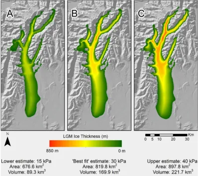
Table 1
Summary of revisions made to LGM outline used in this study. Locations shown inFig. 1. SED¼Surface Exposure Date. Location Description of adjustment (Barrell (2011)as baseline). Basis for adjustment Hope valley 15 km downstream to‘Glenhope’moraines IRSL dating (Rother, 2006)
Waimakariri Valley 20 km downstream to‘Otarama’moraines Mapping and SEDs (Rother et al., 2015)
Rakaia Valley 2 km downstream to‘Tui Creek’moraine crest. SEDs (Shulmeister et al., 2010) and mapping (Soons and
Gullentops, 1973)
Cascade Valley 5 km downstream (to LGM shoreline) Profile of lateral moraine (Sutherland et al., 2007) Upper Clutha Valley (Lake Hawea&Lake
Wanaka)
10 km upstream (to Mt. Iron moraine) IRSL dating (Wyshnytzky, 2013) and radiocarbon dating
(McKellar, 1960).
Milford Sound 3 km upstream (to correspond with submarine terminal moraine)
scenarios;firstly using a‘global’value of 1.75 for all glaciers and
secondly using a‘mid-latitude maritime’value (1.9) for glaciers to
the west of the main divide and a continental mid-latitude value (1.59, derived from the European Alps) for those to the east. The values in the latter scenario were chosen to best accommodate the
east-west climate gradient of the Southern Alps (Henderson and
Thompson, 1999), which is also believed to have been a
promi-nent during the LGM (Drost et al., 2007;Shulmeister et al., 2019).
3. Results
[image:7.595.37.550.543.742.2]3.1. Contemporary lake bathymetry
Table 2details the lakes removed from the DEM and summary
statistics. The location of each lake can be seen onFig. 1. The lakes
have a combined volume of 240.6 km3, highlighting the importance
of their consideration for palaeo ice thickness estimation.
Furthermore, this is thefirst known attempt to quantify the volume
of these lakes, revealing that Lake Wakatipu is volumetrically the
largest (64.2 km3). This is interesting as the title of the‘largest lake
of the South Island’is sometimes noted as Lake Te Anau as it is the
largest by surface area (e.g.McLintock, 1966).
3.2. Shear stress
The vertical extent of LGM glaciation in New Zealand is
unde-fined for the majority of individual catchments. The available
evi-dence, where geomorphological mapping (e.g.Barrell et al., 2011)
has been combined with geochronological dating and some
nu-merical modelling, is summarised inTable 3. This dataset permitted
multiple model runs of varying shear stress to be made of each LGM
glacier to manually best-fit modelled palaeo ice surfaces to that
field-measured and dated. Any surface exposure dates cited
here-after have been recalibrated to the updated production rate from Putnam et al. (2010)in a similar manner to that ofDarvill et al. (2016).
We aimed to generate a profile slightly above the dated
land-form evidence due to the general convex profile of glaciers in the
ablation zone (Nesje, 1992) where centreline ice elevations are
above those on the valley sides, with a differential of 50 m
approximated in previous research deemed appropriate (Glasser
et al., 2011).
The results of the shear stress parameterisation are shown for
each location inFig. 3. A value of 30 kPa best-fitted the available
evidence, providing an acceptablefit to all locations. Since these
catchments include examples from both the east and west of the Main Divide, it appears that for the purposes of our study, a single regionally-averaged value of 30 kPa is appropriate for the entire Southern Alps. Whilst it is acknowledged this approach does not accommodate some inter-catchment variability, we consider it appropriate for our modelling because our aim is to provide geo-metric and volugeo-metric details, rather than information on local ice dynamics or thermal regime, for example.
3.3. Distributed ice thickness and total ice volume
Fig. 4a shows the results of the reconstructed LGM ice thickness across the Southern Alps, with an estimated total volume of
6,800 km3. The REVOLTA model produces large, predominantly
valley-constrained, glaciersflowing to the east of the Main Divide
(e.g. Rakaia and Pukaki Glaciers,Fig. 4b and c) and some piedmont
style glaciers coalescing on the West Coast (e.g. Haast region, Fig. 4d). With the LGM shoreline estimated 125m below present (Milne et al., 2005), only 1 glacier extends marginally past the LGM
coastline (Fig. 4d), accounting for just 0.5 km3of ice (<0.007% of the
total modelled LGM ice volume).
A large number of nunataks are present, especially around the high peaks of the central region. Far fewer nunataks are present south of the Lake Wakatipu region and indeed REVOLTA produces a
localised ice cap in the Fiordland region (Fig. 4e). A maximum
modelled ice thickness of 1,108 m is located at the Wakatipu Glacier (seeFig. 4for location).
3.3.1. Sensitivity analysiseshear stress
We conducted a sensitivity analysis ofTbusing the LGM Pukaki
Glacier as a test case. Analysis was performed for the Pukaki Glacier
due to the abundance of dated landform evidence (Table 3). As
previously noted, the‘bestfit’Tb value of 30 kPa was purposely
chosen to generate a profile slightly above the dated landform
ev-idence. This is due to the general convex profile of glaciers in the
ablation zone (Nesje, 1992) where centreline ice elevations are
above those on the valley sides, with a differential of 50 m
approximated in previous research deemed appropriate (Glasser
et al., 2011). Considering such a convex profile, a‘low’Tbestimate
Table 2
Lakes removed from the contemporary DEM and reference for original source. Summary statistics calculated from interpolated bathymetry.
Lake Name Reference Volume km3 Max depth m Area km2
Te Anau Irwin (1971) 48.25 417 344.2
Hooker Robertson et al. (2012) 0.06 140 1.22
Maud Warren and Kirkbride (1998) 0.08 90 1.40
Godley Warren and Kirkbride (1998) 0.08 90 1.99
Mueller Robertson et al. (2012) 0.02 83 0.87
Pukaki (Irwin, 1970b) 8.9 98 172.8
Rotoroa Irwin (1982b) 2.17 145 23.6
Tasman Dykes et al. (2010) 0.54 240 5.96
Tekapo (Irwin, 1973) 6.94 120 96.5
Monowai Irwin (1981b) 2.56 161 32.0
McKerrow Irwin (1983) 1.69 121 22.9
Manapouri Irwin (1969) 22.47 444 138.6
Kaniere Irwin (1982a) 1.38 198 14.7
Hawea Irwin (1975) 24.49 384 151.7
Hauroko Irwin (1980) 10.97 462 71.0
Ohau (Irwin, 1970a) 4.56 129 59.3
Sumner Irwin (1979) 1.1 134 13.7
Coleridge Flain (1970) 3.65 200 36.9
Brunner Irwin (1981a) 2.24 109 40.6
Wanaka Irwin (1976) 31.92 311 198.9
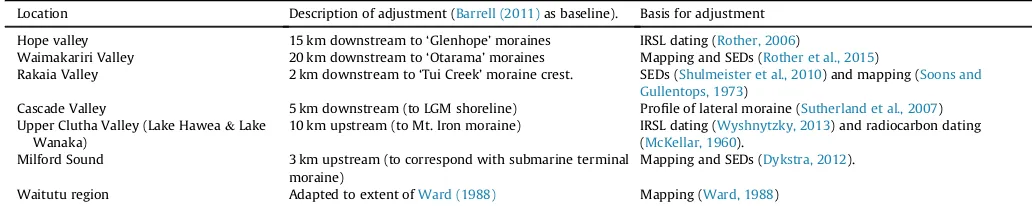
(15 kPa) was used to approximate the lowest elevation landform
evidence whilst a‘high’Tbestimate (40 kPa) was used to exceed the
elevation of the geomorphological evidence by over 50 m.Fig. 5
shows the impact of alteringTbwithin the bounds described: aTb
of 15 kPa (Fig. 5a) produces an area 17.5% less than the ‘bestfit’
30 kPa scenario whilst the 40 kPa scenario (Fig. 5c) produces an
area 9.5% greater than the baseline. For ice volume there was an underestimate of 47.4% (15 kPa model) and an overestimate of 30.5% (40 kPa model). Much of these differences are driven by the
specific topography of the Pukaki Valley, although they provide a
first order estimate of the model sensitivity.
3.3.2. Sensitivity analysisepost LGM sediment infill
Sensitivity analysis was also conducted with regards to post
LGM sediment infill. Analysis was performed for the Pukaki Valley
as this is the only location of the Southern Alps where sufficient
data on sediment thickness exists (McKinnon et al., 2012). Using
the methods described in Section2.1.5.1,Fig. 6a shows the
esti-mated post-LGM sediment thickness distribution (and areal extent)
within the Pukaki Valley, revealing up to 348 m of post-LGM infill.
Modelled LGM ice thickness is shown using the original (no
sedi-ment removed) DEM inFig. 6b and for the newly created‘sediment
removed’version inFig. 6b. Corresponding cross sections of the
LGM bed profile, original DEM and ice surfaces are shown inFig. 6d.
For this modelling, all other parameters were set as per the
stan-dard model (Tbof 30 kPa). When considering overall ice volume in
the study region, modelling with the standard DEM predicts a
volume 4.0 km3(7.3%) lower than that with the sediment removed.
3.4. ELA reconstruction
To compare LGM ELAs with contemporary ELAs, we use a digi-tized version of the contemporary ELA trend surface produced by Chinn and Whitehouse (1980). We use this surface as our baseline
as it is effectively an ELA0surface as most glaciers were close to zero
balance during this period (Chinn et al., 2005).Table 4summarises
the results of the reconstructed LGM ELAs under both balance ratio
scenarios (as described in section2.7) alongside the contemporary
values for corresponding regions, whilstFig. 7graphically displays
the results for the balance ratio 1.9 west/1.59 east scenario. LGM ELAs were substantially lower than present, with regionally aver-aged estimates of approximately 900 m. There was large spatial
variability of ELAs during the LGM, as there is at present (Carrivick
and Chase, 2011), with LGM glaciers flowing to the west coast exhibiting ELAs approximately 320 m lower than those to the east.
A gradual south west e north east trend can also be observed
(Fig. 7a), with the lowest values found in the south west. Super-imposed upon these trends is further local variability, with
localised ELA low points found where additional mountain masses are parallel and offset to the west of the main divide (e.g. Solution
Range, Fig. 7a) whilst higher ELAs are found where low passes
penetrate the main divide (e.g. Hollyford Pass,Fig. 7a). Both balance
ratio scenarios produce similar results, although a marginally stronger east-west differential and associated ELA gradient are evident under the 1.9 west/1.59 east scenario.
LGM ELAs were depressed by approximately 950 m on average, although depressions were greater for glaciers to the west of the main divide (under both balance ratio scenarios). Calculation of average ELA gradients across three transects (as originally used by Chinn and Whitehouse (1980)) reveals that east-west ELA gradients during the LGM were markedly reduced at locations where they are
presently very high (Fig. 7, T2: Mt. Cook and T3: Olivine Range
transects) whilst increasing at the northernmost transect (T1: Whitcombe Pass) where a lower ELA gradient is currently present.
4. Discussion
4.1. Style and nature of glaciation during the LGM
Our estimate of 6,800 km3 ice volume for the Southern Alps
during the LGM is similar to that by Golledge et al. (2012) of
6,400 km3(adjusted herein for the same spatial extent). The
com-parison is especially interesting because of the markedly different
approaches:Golledge et al. (2012)took climate proxy data to drive
an iceflow dynamics model, whereas we utilised geomorphological
evidence of glacier extent to derive distributed glacier ice thickness independent of climate estimates. With current ice volume of
approximately 50 km3(Chinn, 2001), the Southern Alps has lost
approximately 99.25% of its glacial ice since the LGM, highlighting the climatic sensitivity of the glaciers. For comparison, Greenland has lost approximately 36% of its ice since the LGM and Antarctica
just 7% (Bintanja et al., 2002).
There is some debate and uncertainty surrounding the vertical ice extent in New Zealand during the LGM although there is a growing consensus that glaciers were somewhat constrained by
topography and a full ice cap was not present. Anderson and
Mackintosh (2006) suggest the abundance of extremely sharp ridgelines as evidence they were not overridden by ice whilst modelling of individual catchments clearly shows exposed
ridge-lines around the Mt. Cook region (Putnam et al., 2013). Although
the previous regional modelling byGolledge et al. (2012)presents a
continuous‘icefield’style of glaciation, ice thickness over many of
the peaks and ridgelines is actually modelled to be extremely low. The results of REVOLTA in this study are consistent with a valley constrained style of glaciation, with exposed ridges and nunataks,
[image:8.595.45.563.84.215.2]especially in central and northern regions (Fig. 4). The main
Table 3
Locations used for manually parameterising shear stress value for use in REVOLTA. SeeFig. 1for locations. SED¼Surface Exposure Date.
Location Description Reference(s)
Pukaki Valley Clearly defined 40 km lateral moraine sequence constrained to LGM period (18e30 ka) by over 50 SED samples
Doughty et al. (2015) Kelley et al. (2014) Schaefer et al. (2006)
Glaciological model McKinnon et al. (2012)
Ohau Valley Series of SED samples constraining lateral moraines to LGM period (18e30 ka).
Putnam et al. (2013)
Glaciological model Putnam et al. (2013)
Milford Sound Series of SED samples between 8 and 238 m a.s.l. within LGM period (18e30 ka)
Dykstra (2012)
Waimakariri Valley SED samples constraining various geological features to LGM period (18e30 ka)
Rother et al. (2015)
Cascade Valley Clearly defined 13 km long lateral moraine dated to LGM (~21.85 ka) by a series of cosmogenic samples.
Fig. 4.a) REVOLTA derived 100 m resolution simulation of LGM ice thickness for the Southern Alps domain using optimal parameters (Tb¼30 kPa). 3D simulations of: b) Rakaia
exception to this is in the Fiordland region, where REVOLTA
sug-gests a localised ice cap style of glaciation (Fig. 4e). Interestingly,
this pattern is almost identical to that proposed by Chinn et al.
(2014)who postulated that the Darran Range (adjacent to Milford Sound) marked an approximate boundary between a southern ice cap and a northern region where peaks and ridges penetrated the LGM ice.
The REVOLTA modelling approach also provides an indirect insight into potential basal conditions as the parameterisation
scheme forTbeffectively accounts for basal sliding (Veen, 2013).
Specifically, we found aTbvalue of 30 kPa best represented
land-form evidence, with a range between 15 kPa and 40 kPa deemed plausible. If motion was solely by internal deformation we would
expectTbto be around 50e150 kPa (Nye, 1952;Paterson, 1994). As
such, we interpret that basal sliding was prominent for NZ glaciers during the LGM. Whilst this is in agreement with other studies (e.g. Golledge et al., 2012) due to sedimentary and geomorphological
evidence (Mager and Fitzsimons, 2007; Evans et al., 2013),
Shulmeister et al. (2019) suggests this is not always the case. In their study, it is suggested that basal substrate plays a crucial role,
with rapid water drainage through stratified gravels limiting
mo-tion to internal deformamo-tion. Conversely, when the bed consists of a high mud content (e.g. lake basins), rapid basal sliding may occur. Whilst our study supports the notion of generally wet and sliding conditions at the regional scale, further research is needed to quantify variability over space and time.
Whilst the total volume and most of the longitudinal profiles
presented inFig. 3are similar to those ofGolledge et al. (2012), the
Milford profile (Fig. 3e) is markedly different, with differentials of
ice surface elevation in excess of 300 m in places. The good agree-ment between REVOLTA and the (albeit limited) surface exposure dates in this catchment suggests that the results of REVOLTA are the
most plausible in this location. One potential reason forGolledge
et al. (2012)overestimating glacier ice surface elevations and
vol-ume in this specific catchment (compared the age controlled
geomorphological evidence and REVOLTA) is their assumption of spatially-uniform differentials of temperature and precipitation between the LGM and present. This is noted in their analysis, where scenarios which better reproduced known glacial limits to the east of the main divide (e.g. the Rakaia) produced overextended glaciers
in the central west coast areas. In essence, their‘optimal
recon-struction’can be seen as a compromise between under-estimating
certain glaciers to the east of the main divide (as discussed in their
analysis and shown in Fig. 1) and over-estimating those of the
central west coast (as shown inFig. 3e).
4.2. ELA reconstruction and implications for climatic conditions
Our LGM ELA estimates for individual glaciers of between 375 m
and 1,502 m are of a similar range to those reported byGolledge
[image:11.595.93.492.66.420.2]increased east/west differential, as would be expected (Table 4). As the differences are minimal, we suggest that either scenario is appropriate for the purposes of our modelling, although the 1.9 west/1.59 east scenario may be preferred as this better represents
the known conditions of the glaciers currently in the region (Chinn
et al., 2005). Importantly, the global scenario (balance ratio for all
glaciers¼1.75) still reproduces a strong west-east differential, so
we can be confident that this differential is not due to the choice of
balance ratios on each side of the main divide.
A high east-west ELA gradient has long been recognized be-tween contemporary Southern Alps glaciers and is often
inter-preted as a response to the current precipitation pattern (Porter,
1975a). As such we infer the presence of an east-west ELA gradient during the LGM as evidence that westerly circulation was in operation to some extent during the LGM, a view shared by other
[image:12.595.107.502.64.468.2]authors (e.g.Rother and Shulmeister, 2006). Crucially however, our
Fig. 6.a) Estimated areal extent and thickness of post LGM-sediment in the Pukaki basin. b) Modelled ice thickness (standard DEM). c) Modelled ice thickness (sediment removed DEM). d) Cross-section of M1-M2 transect.
Table 4
Contemporary and LGM ELAs for the Southern Alps, associated depression during the LGM and east-west gradients. SeeFig. 7a for location of transects. Contemporary LGM
balance ratio 1.75 balance ratio 1.9 west/1.59 east
Mean (entire) 1,849 m 900 m 898 m
Mean (east) 1,976 m 1,087 m 1,100 m
Mean (west) 1,681 m 774 m 760 m
Depression from contemporary (entire) 949 m 951 m Depression from contemporary (east) 889 m 876 m Depression from contemporary (west) 907 m 921 m ELA gradient, transect T1 (Whitcombe Pass) 3.7 m/km1 11.6 m/km1 12.6 m/km1
ELA gradient, transect T2 (Mt. Cook Region) 31 m/km1 13.5 m/km1 14.0 m/km1
[image:12.595.41.562.530.639.2]results show that there was spatial variability in the ELA depression and associated gradients, suggesting that climatic change was not
uniform across the Southern Alps. Analysis of the‘Mt. Cook’and
‘Olivine Range’ transects (Fig. 7) shows that LGM ELA gradients
were markedly reduced compared to present (reducing from 31 to
14 m/km1 and 20 and 12.5 m/km1 respectively) whilst the
currently low ELA gradient at the Whitcombe Pass (3.7 m/km1)
was enhanced during the LGM to 12.6 m/km1.
Our assertion of spatial variability in climatic change is in line with a growing body of evidence from other studies using a variety
of techniques, although to our knowledge this study is thefirst to
use glacial reconstruction for such a purpose in New Zealand. McKinnon et al. (2012)collated estimates of temperature deviation
(for the New Zealand LGM) from different studies,finding a large
range in reported values. For example,Sikes et al. (2002)found that
sea surface temperature south of Chatham rise were 8C cooler
than present whilst Marra et al. (2006) inferred very moderate
cooling in the Canterbury region, as little as 2C on average (albeit
probably during a short inter-stadial within the extended LGM). The notion of spatial variability is supported by climate modelling byDrost et al. (2007)who estimated that temperature reduction
varied spatially between 2.5C and 4C from pre-industrial levels.
Although LGM precipitation estimates are less well constrained than temperature, there is evidence to suggest that both the
amount and distribution were significantly different from present.
Palaeo-vegetation studies suggest a major reorganization of vege-tation patterns during the New Zealand LGM, with a general
consensus of drier conditions overall (McGlone et al., 1993).
Pre-cipitation patterns were also likely to be different during the LGM,
with recent research by Shulmeister et al. (2019) postulating
changes driven by a shift in the track of westerlies. Precipitation
modelling byDrost et al. (2007) also supports the concept of a
generally drier climate, albeit with substantial local variation.
Most recently, downscaled climate modelling byKarger et al.
(2017) and Brown et al. (2018) has produced high resolution (~1 km) gridded estimates of LGM mean annual temperature and
precipitation, which were downloaded fromwww.paleoclim.org.
Fig. 8a displays the mean annual temperature distribution at the
LGM using the CCSM4 model, whilst Fig. 8b shows the
corre-sponding values at present (Landcare Research Ltd, 2003b). Similar
maps are shown for precipitation distribution, withFig. 8c showing
the modelled LGM distribution and Fig. 8d showing the
contemporary distribution (Landcare Research Ltd, 2003a). By
dif-ferencing the LGM estimates and corresponding contemporary datasets, the differentials can be calculated for both temperature (Fig. 8e) and precipitation (Fig. 8f). Note that LGM glaciers are
delineated inFig. 8e as no correction has been made for changes in
ice surface elevation and associated effect of lapse rate. Importantly,
the downscaling precipitation algorithm used by Karger et al.
(2017)andBrown et al. (2018)incorporates orographic predictors
including windfields, valley exposition, and boundary layer height,
with a subsequent bias correction. We are therefore confident that
the modelled precipitation data (Fig. 8c) adequately captures the
magnitude of orographic precipitation enhancement in the high-relief setting of the Southern Alps.
These new, high resolution datasets form an independent source for assessing the spatial variability of climatic parameters. Fig. 8e and f demonstrates that changes in temperature and pcipitation distribution varied spatially, as predicted by the ELA
re-constructions of this study (Fig. 7).Fig. 8e shows the majority of the
Southern Alps experienced cooling in the range of 2e5C, broadly
similar to the New Zealand average of 4.6C reported byDrost et al.
(2007)although perhaps slightly lower than the 6.5C suggested byGolledge et al. (2012). Whilst the negligible cooling estimated in north-west regions is surprising, this is within the ranges reported
in the literature, withMarra et al. (2006)suggesting a temperature
increaseof up to 0.5C during summer LGM interstadials at Lyndon
Stream (seeFig. 8e for location) whilstSamson et al. (2005)
re-ported winter sea surface temperature decreases of just 0.9C
(offshore of New Zealand North Island).
For precipitation,Fig. 8f shows major changes in the amount and
distribution during the LGM. Whilst an east-west precipitation
gradient is clearly still modelled during the LGM (Fig. 8c), this is
much reduced, with less precipitation on the west coast, which
currently has some of the highest rainfall on Earth (Henderson and
Thompson, 1999). The pattern is consistent with the assertion of an
overall drier conditions during the LGM (McGlone et al., 1993;Drost
et al., 2007).Drost et al. (2007)also found the greatest precipitation decreases in Western regions, with average reductions of 30% (from pre-industrial levels) in Southern Otago-Southland regions.
In essence, the climate model estimates based on the work of Karger et al. (2017)andBrown et al. (2018)are in correspondence
with the results from the ELA reconstructions in this study (Fig. 7a):
gradient with substantial local level variability. The agreement is especially interesting because of the markedly different
ap-proaches:Karger et al. (2017)andBrown et al. (2018)used a global
climate model to estimate temperature and precipitation wheras we utilised geomorphological evidence to derive ice thickness and associated ELAs.
5. Conclusions
In this study we used geomorphological and geochronological records from the Southern Alps of New Zealand to drive a glacial reconstruction model (REVOLTA) for the LGM. We modelled a total
volume of 6,800 km3of glacier ice across the Southern Alps during
the LGM, representing a 99.25% volume loss to present. Analysis of
the distributed ice thickness reveals a‘valley-constrained' style of
glaciation with many exposed ridges and nunataks, even when
parameterised tofit the maximum vertical extent of
geomorpho-logical evidence. An ice-cap style of glaciation was predicted for the Fiordland region, where maximum surface elevations are lower. We found a low shear stress value of approximately 30 kPa was
required to bestfit the geomorphological evidence, from which we
infer that at least some glaciers were warm-based during the LGM. Reconstructed ELAs reveal a regionally averaged depression of approximately 950 m during the LGM. This ELA depression is
consistent withfindings of other studies. However, and crucially,
we found substantial spatial variability in ELA depression, with east-west ELA gradients during the LGM generally decreased. In conjunction with evidence from the latest independent climate
models (Karger et al., 2017;Brown et al., 2018), we propose that
westerly circulation was decreased during the LGM compared to at present, resulting in decreased precipitation to the west of the main
divide.
The recognition of spatially variable climatic differentials is important because they have not been previously considered when reconstructing LGM ice thickness in New Zealand. Namely, the only
previous such model byGolledge et al. (2012)assumed
spatially-uniform differentials of temperature and precipitation between
the LGM and present. Whilst producing an acceptablefit at the
regional scale, they were unable to resolve known ice limits in some catchments (by up to 40 km). We suggest that some of these anomalies may be due to the use of unrealistic uniform climate differentials, especially precipitation distribution to which glaciers
of the Southern Alps are known to be highly sensitive (Rowan et al.,
2014). The advent of independent high resolution estimates of
palaeo climatic conditions (Karger et al., 2017;Brown et al., 2018)
may help to address some of these issues, allowing further
differ-ences between ‘top down’ climate based reconstructions and
‘bottom up’landform based reconstructions (e.g. REVOLTA) to be
assessed in more detail. The framework presented here could easily be applied to other formerly glaciated regions, helping to improve our knowledge of the global climate system.
Acknowledgements
WJ was funded by a NERC PhD studentship (NE/K500847/1). JC and WJ thanks the School of Geography, University of Leeds, for
assistance with fieldwork costs. Trevor Chinn commented on an
early version of the manuscript.
Appendix A. Supplementary data
[image:14.595.112.499.70.368.2]https://doi.org/10.1016/j.quascirev.2019.06.035.
References
Adams, J., 1980. Contemporary uplift and erosion of the southern Alps, New
Zea-land’. Geol. Soc. Am. Bull. 91, 1e114.
Alexander, D., Davies, T., Shulmeister, J., 2014. Formation of the Waiho Loop
ter-minal moraine, New Zealand. J. Quat. Sci. 29, 361e369.
Anderson, B.M., Hindmarsh, R.C.A., Lawson, W.J., 2004. A Modelling Study of the
Response of Hatherton Glacier to Ross Ice Sheet Grounding Line Retreat’, Global
and Planetary Change, vol. 42. Elsevier, pp. 143e153, 1e4.
Anderson, B., Mackintosh, A., 2006. Temperature change is the major driver of
late-glacial and Holocene glacierfluctuations in New Zealand. Geology 34, 121e124.
Barrell, D.J.A., Andersen, B.G., Denton, G.H., Smith Lyttle, B., 2011. Glacial Geo-morphology of the Central South Island, New Zealand, vol. 27. GNS Science
monograph.
Barrell, D.J.A., 2011. Quaternary glaciers of New Zealand. In: Ehlers, J., Gibbard, P.,
Hughes, P. (Eds.), Developments in Quaternary Science. Elsevier, Amsterdam.
Beavan, J., Ellis, S., Wallace, L., Denys, P., 2007.‘Kinematic Constraints from GPS on
Oblique Convergence of the Pacific and Australian Plates, Central South Island,
New Zealand’, vol. 175. Geophysical Monograph Series, pp. 75e94.
Benn, D.I., Hulton, N.R.J., 2010. An Excel (TM) spreadsheet program for
recon-structing the surface profile of former mountain glaciers and ice caps. Comput.
Geosci. 36, 605e610.
Bintanja, R., Van de Wal, R.S.W., Oerlemans, J., 2002. Global ice volume variations through the last glacial cycle simulated by a 3-D ice-dynamical model. Quat. Int.
95, 11e23.
Brown, J.L., Hill, D.J., Dolan, A.M., Carnaval, A.C., Haywood, A.M., 2018. PaleoClim, High Spatial Resolution Paleoclimate Surfaces for Global Land Areas, vol. 5.
Scientific data, 180254.
Burdis, A.J., 2014. Denudation Rates Derived from Spatially-Averaged Cosmogenic Nuclide Analysis in Nelson/Tasman Catchments, South Island, New Zealand.
PhD thesis. University of Wellington.
Carrivick, J.L., Davies, B.J., James, W.H.M., Quincey, D.J., Glasser, N.F., 2016. Distrib-uted ice thickness and glacier volume in southern South America. Global and
Planetary Change 146, 122e132.
Carrivick, J.L., Davies, B.J., James, W.H.M., McMillan, M., Glasser, N.F., 2019. A comparison of modelled ice thickness and volume across the entire Antarctic
Peninsula region, Geografiska Annaler: Series A. Physical Geography 101 (1),
45e67.
Carrivick, J.L., Boston, C.M., King, O., James, W.H.M., Quincey, D.J., Smith, M.W., Grimes, M., Evans, J., 2019. Accelerated volume loss in glacier ablation zones of NE Greenland, Little Ice Age to present. In: Geophysical Research Letters, vol. 46. American Geophysical Union.https://doi.org/10.1029/2018GL081383.
Carrivick, J.L., Chase, S.E., 2011. Spatial and temporal variability in the net mass balance of glaciers in the Southern Alps, New Zealand. N. Z. J. Geol. Geophys. 54,
415e429.
Chinn, T., Kargel, J.S., Leonard, G.J., Haritashya, U.K., Pleasants, M., 2014. New Zea-land's glaciers. In: JS, K., et al. (Eds.), Global Land Ice Measurements from Space.
Praxxis, Chichester.
Chinn, T.J., 2001. Distribution of the glacial water resources of New Zealand.
J. Hydrol. (New Zealand) 40, 139e187.
Chinn, T.J.H., Whitehouse, I.E., 1980.‘Glacier Snow Line Variations in the Southern
Alps, New Zealand’,World Glacier Inventory, vol. 126. International Association
of Hydrological Sciences Publication, pp. 219e228.
Chinn, T.J., Heydenrych, C., Salinger, M.J., 2005.‘Use of the ELA as a practical method
of monitoring glacier response to climate in New Zealand's Southern Alps'.
J. Glaciol. 51, 85e95.
Coates, G., 2002. The Rise and Fall of the Southern Alps. Canterbury University
Press, Christchurch.
Darvill, C.M., Bentley, M.J., Stokes, C.R., Shulmeister, J., 2016. The timing and cause of glacial advances in the southern mid-latitudes during the last glacial cycle based on a synthesis of exposure ages from Patagonia and New Zealand. Quat.
Sci. Rev. 149, 200e214.
Doughty, A.M., Schaefer, J.M., Putnam, A.E., Denton, G.H., Kaplan, M.R., Barrell, D.J.A., Andersen, B.G., Kelley, S.E., Finkel, R.C., Schwartz, R., 2015. Mismatch of glacier extent and summer insolation in Southern Hemisphere mid-latitudes. Geology
43, 407e410.
Drost, F., Renwick, J., Bhaskaran, B., Oliver, H., McGregor, J., 2007.‘A simulation of
New Zealand's climate during the Last Glacial Maximum’. Quat. Sci. Rev. 26,
2505e2525.
Dykes, R.C., Brook, M.S., Winkler, S., 2010. The contemporary retreat of Tasman Glacier, Southern Alps, New Zealand, and the evolution of Tasman proglacial
lake since AD 2000. Erdkunde 64, 141e154.
Dykstra, J., 2012. The Role of Mass Wasting and Ice Retreat in the Post-LGM Evo-lution of Milford Sound, Fiordland, New Zealand. PhD thesis. University of
Canterbury, New Zealand.
Evans, D.J.A., Rother, H., Hyatt, O.M., Shulmeister, J., 2013. The glacial sedimentology and geomorphological evolution of an outwash head/moraine-dammed lake,
South Island, New Zealand. Sediment. Geol. 284, 45e75.
Finlayson, A., 2013. Digital surface models are not always representative of former glacier beds: palaeoglaciological and geomorphological implications.
Geo-morphology 194, 25e33.
Flain, M., 1970. Lake Coleridge Bathymetry, 1:23. New Zealand Oceanographic
Institute Chart Series, p. 760.
Geographix, 2012. NZ 8m Digital Elevation Model.www.geographx.co.nz. (Accessed January 2018).
Glasser, N.F., Harrison, S., Jansson, K.N., Anderson, K., Cowley, A., 2011. Global
sea-level contribution from the patagonian icefields since the little ice age
maximum. Nat. Geosci. 4, 303e307.
Golledge, N.R., Mackintosh, A.N., Anderson, B.M., Buckley, K.M., Doughty, A.M., Barrell, D.J.A., Denton, G.H., Vandergoes, M.J., Andersen, B.G., Schaefer, J.M., 2012. Last glacial maximum climate in New Zealand inferred from a modelled
southern Alps icefield. Quat. Sci. Rev. 46, 30e45.
Harbor, J.M., Wheeler, D.A., 1992. On the mathematical description of glaciated
valley cross sections. Earth Surf. Process. Landforms 17, 477e485.
Henderson, R.D., Thompson, S.M., 1999. Extreme rainfalls in the southern Alps of
New Zealand. J. Hydrol. (New Zealand) 38, 309e330.
Heron, D.W., 2014. ‘Geological Map of New Zealand 1:250 000’, GNS Science
Geological Map 1. GNS Science, New Zealand. Lower Hutt.
Hinderer, M., 2001. Late Quaternary denudation of the Alps, valley and lakefillings
and modern river loads. Geodin. Acta 14, 231e263.
Hutchinson, M.F., 1989. A new procedure for gridding elevation and stream line
data with automatic removal of spurious pits. J. Hydrol. 106, 211e232.
Irwin, J., 1969. Lake Manapouri Bathymetry, 1:31,680. New Zealand Oceanographic
Institute Chart Series.
Irwin, J., 1970a. Lake Ohau Bathymetry, 1:31,680. New Zealand Oceanographic
Institute Chart Series.
Irwin, J., 1970b. Lake Pukaki bathymetry, 1:31,680. New Zealand Oceanographic
Institute Chart Series.
Irwin, J., 1971. Lake Te Anau Bathymetry, 1:63,360. New Zealand Oceanographic
Institute Chart Series.
Irwin, J., 1972. Lake Wakatipu Bathymetry, 1:63,360. New Zealand Oceanographic
Institute Chart Series.
Irwin, J., 1973. Lake Tekapo Bathymetry, 1:31,680. New Zealand Oceanographic
Institute Chart Series.
Irwin, J., 1975. Lake Hawea Bathymetry, 1:47,520. New Zealand Oceanographic
Institute Chart Series.
Irwin, J., 1976. Lake Wanaka Bathymetry, 1:55,440. New Zealand Oceanographic
Institute Chart Series.
Irwin, J., 1979. Lake Sumner, Katrine, Mason and Marion Bathymetry, 1:12,000. New
Zealand Oceanographic Institute Chart Series.
Irwin, J., 1980. Lake Hauroko Bathymetry, 1:30,000. New Zealand Oceanographic
Institute Chart Series.
Irwin, J., 1981a. Lake Brunner Bathymetry, 1:15,000. New Zealand Oceanographic
Institute Chart Series.
Irwin, J., 1981b.‘Lake Monowai Bathymetry, 1:20,877’. New Zealand Oceanographic
Institute Chart Series.
Irwin, J., 1982a. Lake Kaniere Bathymetry, 1:12,000. New Zealand Oceanographic
Institute Chart Series.
Irwin, J., 1982b. Lake Rotoroa Bathymetry, 1:15,840’. New Zealand Oceanographic
Institute Chart Series.
Irwin, J., 1983. Lake McKerrow and Lake Alabaster Bathymetry, 1:18,000. New
Zealand Oceanographic Institute Chart Series.
Jaboyedoff, M., Derron, M.-H., 2005. A new method to estimate the infilling of
al-luvial sediment of glacial valleys using a sloping local base level. Geografia
Fisica e Dinamica Quaternaria 28, 37e46.
James, W.H., Carrivick, J.L., 2016. Automated modelling of distributed glacier ice
thickness and volume. Comput. Geosci. 92, 90e103.
James, W.H.M., 2016. A Landform Based 3D Reconstruction of Glacier Ice at the Last Glacial Maximum the Southern Alps, New Zealand. PhD Thesis. University of
Leeds.
Kamp, P.J.J., Green, P.F., White, S.H., 1989. Fission track analysis reveals character of
collisional tectonics in New Zealand. Tectonics 8, 169e195.
Karger, D.N., Conrad, O., Bohner, J., Kawohl, T., Kreft, H., Soria-Auza, R.W.,€
Zimmermann, N.E., Linder, H.P., Kessler, M., 2017. Climatologies at High
Reso-lution for the Earth's Land Surface Areas, vol. 4. Scientific data. Nature
Pub-lishing Group (170122).
Kelley, S.E., Kaplan, M.R., Schaefer, J.M., Andersen, B.G., Barrell, D.J.A., Putnam, A.E., Denton, G.H., Schwartz, R., Finkel, R.C., Doughty, A.M., 2014. High-precision 10Be chronology of moraines in the Southern Alps indicates synchronous cooling in Antarctica and New Zealand 42,000 years ago. Earth Planet. Sci. Lett.
405, 194e206.
Landcare Research Ltd, 2003a. Mean Annual Precipitation Dataset.www.lris.scinfo.
org.nz. (Accessed March 2018).
Landcare Research Ltd, 2003b. Mean Annual Temperature Dataset.www.lris.scinfo.
org.nz. (Accessed August 2018).
Levy, R.H., Dunbar, G., Vandergoes, M., Howarth, J.D., Kingan, T., Pyne, A.R., Brotherston, G., Clarke, M., Dagg, B., Hill, M., 2018. A High-Resolution Climate Record Spanning the Past 17 000 Years Recovered from Lake Ohau, South Island,
New Zealand. Scientific Drilling.
Li, H., Ng, F., Li, Z., Qin, D., Cheng, G., 2012. An extended“perfect-plasticity”method for estimating ice thickness along theflow line of mountain glaciers. J. Geophys. Res. 117 (F1)https://doi.org/10.1029/2011jf002104.
Linsbauer, A., Paul, F., Haeberli, W., 2012. Modeling glacier thickness distribution and bed topography over entire mountain ranges with GlabTop: application of a fast and robust approach. J. Geophys. Res. 117 (F3) https://doi.org/10.1029/
2011JF002313.