sampling
.
White Rose Research Online URL for this paper:
http://eprints.whiterose.ac.uk/144212/
Version: Published Version
Article:
Chang, Wanli orcid.org/0000-0002-4053-8898, Goswami, Dip, Chakraborty, Samarjit et al.
(1 more author) (2018) OS-aware automotive controller design using non-uniform
sampling. ACM Transactions on Cyber-Physical Systems. 26. ISSN 2378-9638
https://doi.org/10.1145/3121427
[email protected] https://eprints.whiterose.ac.uk/ Reuse
Items deposited in White Rose Research Online are protected by copyright, with all rights reserved unless indicated otherwise. They may be downloaded and/or printed for private study, or other acts as permitted by national copyright laws. The publisher or other rights holders may allow further reproduction and re-use of the full text version. This is indicated by the licence information on the White Rose Research Online record for the item.
Takedown
If you consider content in White Rose Research Online to be in breach of UK law, please notify us by
26
Non-Uniform Sampling
WANLI CHANG
,Singapore Institute of TechnologyDIP GOSWAMI
,Eindhoven University of TechnologySAMARJIT CHAKRABORTY
,Technical University of MunichARNE HAMANN
,Robert Bosch GmbHAutomotive functionalities typically consist of a large set of periodic/cyclic tasks scheduled under a real-time operating system (OS). Many of the tasks are feedback control applications with stringent performance requirements. OSEK/VDX is a common class of automotive OS that ofers preemptive periodic schedules supporting a pre-conigured set of periods. The feedback controllers implemented onto such OSEK/VDX-compliant systems need to use one of the pre-conigured (sampling) periods. A shorter period is often de-sired for a higher control performance, and this implies a higher processor load. For a given performance requirement, the longest sampling period that meets this requirement is the optimal one. Given a limited set of pre-conigured periods, such optimal sampling periods are often not available, and the practice is to choose a shorter available period—leading to a higher processor load. To address this, we propose a controller that cyclically switches among the available periods, thereby leading to an average sampling period closer to the optimal one. This way, we reduce the processor load and are able to pack more control applications on the same processor. The main challenge in this article is the design of such controllers that takes into account such cyclic switching of sampling periods (i.e., use non-uniform sampling). The controller needs to meet speciied performance requirements (settling time) and system constraints (e.g., input saturation). Such a non-convex constrained controller optimization problem as raised in the OS-aware automotive systems design has not been addressed in the traditional optimal control literature. A novel approach based on adaptively parame-terized particle swarm optimization (PSO) is proposed to solve it. Using the OS-aware controller design with non-uniform sampling, we show that a higher number of applications can be packed on a processor, which is of particular interest in the cost-sensitive automotive industry.
CCS Concepts: •Computer systems organization→Embedded and cyber-physical systems; Real-time operating systems;
Additional Key Words and Phrases: OSEK/VDX, non-uniform sampling, computation resources, optimal control
ACM Reference format:
Wanli Chang, Dip Goswami, Samarjit Chakraborty, and Arne Hamann. 2018. OS-Aware Automotive Contro-ller Design Using Non-Uniform Sampling.ACM Trans. Cyber-Phys. Syst.2, 4, Article 26 (July 2018), 22 pages.
https://doi.org/10.1145/3121427
This work is partially supported by the Singapore National Research Foundation under its Campus for Research Excellence And Technological Enterprise (CREATE) program.
Authors’ addresses: W. Chang, Singapore Institute of Technology, 10 Dover Drive, Singapore 138683; email: wanli.chang@ singaporetech.edu.sg; D. Goswami, Eindhoven University of Technology, P.O. Box 513, 5600 MB Eindhoven, The Nether-lands; email: [email protected]; S. Chakraborty, Technical University of Munich, Arcisstrasse 21, D-80290, Munich, Ger-many; email: [email protected]; A. Hamann, Robert Bosch GmbH, Renninger, 70465 Stuttgart, GerGer-many; email: arne. [email protected].
Permission to make digital or hard copies of all or part of this work for personal or classroom use is granted without fee provided that copies are not made or distributed for proit or commercial advantage and that copies bear this notice and the full citation on the irst page. Copyrights for components of this work owned by others than ACM must be honored. Abstracting with credit is permitted. To copy otherwise, or republish, to post on servers or to redistribute to lists, requires prior speciic permission and/or a fee. Request permissions [email protected].
1 INTRODUCTION
In the past decade, the complexity of automotive software and the number of applications and software tasks have considerably increased. For instance, in engine management, the main drivers are complex exhaust gas treatment systems like NOx storage catalyst converter (NSC) and selec-tive catalytic reduction (SCR) and fuel eiciency measures like staged injection and variable cam timing (Jeong et al. 2011; Popovic et al. 2003). As a consequence, standard engine management software nowadays contains dozens of tasks with around 1,500 runnables (Kramer et al.2015). At the same time, automotive systems are highly cost sensitive, and there is an increasing efort to in-tegrate multiple tasks onto a single electronic control unit (ECU). In line with such developments, in this article we study a commonly occurring setup—where multiple feedback control applica-tions are to be implemented on a single ECU. The goal is to pack as many applicaapplica-tions as possible in an efort to reduce costs.
Tasks in automotive software systems are typically scheduled with preemptive policies and cyclically repeated with a ixed period on OSEK/VDX-compliant operating systems (OS)1(Feiler 2003; Consortium 2005; Apuzzo et al.2016). For control applications, runnables containing the functional code are assigned to tasks according to the continuous dynamics of the physical process being controlled. For example, injection control in engine management has faster dynamics than exhaust gas control and thus requires a shorter period.
A feedback control loop consists of three operations:
—Measure:Sensors measure the states of the physical plants. This is also called sampling. —Compute:Taking the data from sensors, control programs are executed and compute the
control input.
—Actuate:The control input is sent to actuators, aiming to achieve certain desired behavior of the plants.
In this work, we assume that the measure and the actuate operations take negligible time compared to the compute operation, and they are performed in a separate sensing/actuating unit under a strict time-triggered policy. As shown in Figure1, the time duration between two consecutive measurements (or samplings) of the plant states is deined as the sampling periodh. The time duration between the measurement and the actuation of one feedback control loop is deined as the sensor-to-actuator delayτsa. The actual execution time of the control program is denoted as Eand the worst-case execution time (WCET) isEwc. The actuate operation is performed exactly afterEwctime from the measure operation while the compute operation is performed in between. This setting leads to a constant sensor-to-actuator delay, i.e.,τsa=Ewc.
Generally, a shorter sampling period allows the controller to respond to its plant more frequently and is thus potentially able to achieve a better control performance with an appropriately designed controller. The obvious downside is a higher processor load, since the control program is executed more frequently. This prevents more functions and applications from being integrated onto the ECU. Therefore, the controller should be designed to use the largest possible sampling period (to reduce ECU load) that is able to fulill the control performance requirement and satisfy the system constraints. This is theoptimalsampling period that should be ideally used.
Fig. 1. The general timing model of a control loop.
Fig. 2. Allowed switching instants among multiple sampling periods.
Fig. 3. Packing of control applications onto the ECU.
However, an OSEK/VDX OS is usually pre-conigured to support a small set of predeined sam-pling periods.2Hence, often the optimal sampling period is not directly realizable on the ECU. The conventional way to handle it is to use the largest sampling period from the pre-conigured set of sampling periods available in the OSEK/VDX OS that is shorter than the optimal one. It is clearly a waste of scarce computation resources on board.
Main idea:In this work, we design controllers thatswitchbetween the available pre-conigured sampling periods ofered by the OSEK/VDX OS, following a predeined static schedule. A typical example with sampling periods of 2, 5, and 10ms on OSEK/VDX OS is illustrated in Figure2. For one application, switching between two sampling periods can only occur at the common multiplier of them. For instance, switching between 2 and 5ms is possible at the time instant of 10ms, 20ms, and so on. Therefore, possible sequences of sampling periods are {2ms, 2ms, 2ms, 2ms, 2ms, 5ms, 5ms, repeat}, {5ms, 5ms, 10ms, repeat}, and so on.
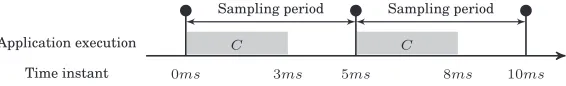
Illustrative example:We now explain a simple case that multiple identical control applications C need to be implemented on ECUs. Assuming that the control performance requirement ofC can be satisied with a sampling period of 5ms, yet not with 10ms. If the WCET ofCis 3ms, then only one application can be implemented on the ECU as shown in Figure3, since the sampling
[image:4.486.102.385.342.385.2]period 5ms is not long enough to execute two applications, which require 6ms. If 10ms is used as the sampling period, then three applications can be integrated into the ECU. However, this is not feasible due to the violation of the control performance requirement. A non-uniform sampling schedule {5ms, 5ms, 10ms, repeat} achieves an average sampling period of 6.67ms, which reduces the processor load compared to the schedule with a constant sampling period of 5ms and enables two applications to be packed onto the ECU. Detailed scheduling will be explained later in this article. The question is how to design the controller for such a non-uniform sampling schedule to satisfy the control performance requirement.
Contributions:The main technical challenge we address is designing a controller that uses a non-uniform scheme, striving for optimizing control performance and respecting system constraints simultaneously to pack more control applications on one processor. Given a non-uniform sampling schedule, which could come up by checking the performance of uniform sampling schedules, our proposed controller design approach optimizes the settling time—a common control performance metric that is especially important for real-time applications and harder to analyze than quadratic cost and explicitly respects the hard physical constraint on the input saturation. Such a constrained non-convex optimization problem with signiicant non-linearity has not been addressed in the control theory literature and does not lend itself to an analytical closed-form solution. Therefore, one has to resort to heuristic optimization techniques. In this article, we address this problem using an approach based on particle swarm optimization (PSO) with adaptive parameterization for controller pole-placement. The proposed idea is evaluated on a real-life electro-mechanical braking (EMB) system. The number of applications implemented on an ECU can be higher, which makes the presented approach attractive for the cost-sensitive automotive domain.
Although the OS-related constraints are a major problem faced in the industry when designing embedded control systems, currently there are no systematic solutions. This is the irst article that provides a solution to handle OS-related characteristics directly in the control strategy. While there have been works taking network characteristics or communication resources into account when designing controllers (Hong et al.2010,2015; Chen et al.2014), in many embedded systems, computation resources are often also scarce (due to the use of simple microcontrollers and cost pressures). Our work goes in this direction and the techniques we provide result in computation-resource-eicient controllers.
Organization:The rest of the article is organized as follows. Section2discusses the related work on resource-aware embedded control systems design, optimal control and non-uniform sampling. Section3describes the automotive system architecture under consideration, including feedback control applications and the OSEK/VDX OS. The OS-aware controller design is presented in Sec-tion4. A novel PSO technique with adaptive parameterization is proposed in Section5to solve the pole-placement problem. Section6introduces an alternative controller design with better scala-bility. Experimental results on the EMB system are reported in Section7, and Section8makes the concluding remarks.
2 RELATED WORK
illustrated on a train car. In Yue et al. (2013), a delay system model is constructed by investigating the efect of the network transmission delay. A novel event-trigger controller that co-designs the feedback gain and the trigger parameters is proposed and shown to have superior performance with simulation results. A co-optimization approach, which synthesizes both the controllers and communication schedules for FlexRay-based distributed control systems, is reported in Roy et al. (2016). The scalability issue is addressed and the tradeof between control performance and bus utilization ofers lexibility to designers.
Computation resources have been taken into account in only a few works (Castane et al.2006; Greco et al.2011; Cervin et al.2002). A resource management strategy adjusting the task periods at runtime considering the response over a inite time horizon of the plants is proposed in Castane et al. (2006) to maximize the control performance. In Greco et al. (2011), a novel controller design technique based on a hierarchy of controllers is proposed, so that when the allocated execution time is short, a low-level computationally light controller is activated to achieve basic control per-formance and when the execution time is long, a high-level computationally intensive controller is used aiming for better control performance. In Cervin et al. (2002), a scheduling architecture for real-time control tasks is proposed. The scheduler uses feedback from execution time mea-surements and feedforward from workload changes to adjust the sampling periods of the control tasks so that the combined performance (a linear or quadratic cost function) of the controllers is optimized. None of the eforts above address the restriction from the OS.
Works in control theory literature with non-uniform sampling and switched systems focus on guaranteeing stability (Lin and Antsaklis2009; Lemmon and Hu2011). Generally, theoretical tools such as common quadratic Lyapunov functions (CQLF) and switched Lyapunov functions (SLF) tackle arbitrary switching between sampling periods to assure stability of the overall closed-loop system. In our work, as opposed to arbitrary switching, the sequence of sampling periods is cyclic and decided in the design phase. We aim for further performance optimality by exploiting this additional knowledge about the switching behavior. In the ield of optimal control, techniques such as linear quadratic regulator (LQR) and its variants (e.g., periodic LQR) (Lavretsky and Wise 2013) are well developed. However, they do not explicitly consider the hard constraint on the control input, which exists in most real-life control applications such as automobiles.
The combination of performance optimization and input constraint satisfaction is addressed by model predictive control (MPC) techniques (Rawlings and Mayne2009)—another well-developed area. MPC performs online optimization in every sampling period, making it computationally heavy and unsuitable for being implemented on the resource-constrained embedded platform, which is what we are studying in this work. Explicit MPC pre-optimizes the controller for all pos-sible system states and searches for the optimal control input from a look-up table online. These existing optimal control methods cannot be directly applied in our work, since their optimization objective is quadratic cost. Considering both settling time and input saturation simultaneously, which are non-convex on the controller poles is particularly challenging and will be addressed in this work.
Online optimal sampling period assignment is investigated in Cervin et al. (2011) to maximize the control performance. A feedback scheduler is developed to periodically assign new sampling periods based on the current plant states. It is shown that most computation can be done oline and stored in a look-up table. Again, only the quadratic cost function is considered and the selection of sampling periods is not restricted. Besides, since the switching is not ixed, yet occurs depending on the plant states in real time, stability cannot be guaranteed. Building on these previous works, our method formulates an optimal pole-placement problem for a non-uniform schedule known in the design phase, where the input saturation is explicitly respected, the settling time is minimized, and the stability is ensured.
3 SYSTEM ARCHITECTURE
We consider a typical automotive setup that multiple feedback control applications share an ECU with other applications. The ECU runs OSEK/VDX OS. The two main elements of such a system architecture—feedback control applications and the OSEK/VDX OS—are described in this section.
3.1 Feedback Control Applications
Plant dynamics:A control application is responsible for controlling a plant or a dynamic system. In particular, we consider linear single-input-single-output (SISO) control applications where the dynamic behavior is modeled by a set of diferential equations,
˙
x(t) =Ax(t)+Bu(t),
y(t) =Cx(t), (1)
wherex(t)∈Rn is thesystem state, ˙x(t)is the derivative ofx(t)with respect to time,y(t) is the
system output, andu(t) is thecontrol inputapplied to the system. The number of system states is n. Thesystem matrix(orstate matrix) isA, theinput matrixisB, and theoutput matrixisC. These matricesA,B, andCcapture physical properties of the plant. System poles are eigenvalues ofA.
Discretized dynamics:In most applications, the controller is implemented in a digital fashion on a computer. This implies that the system states must be sampled when measured by the sensors, as has been shown in Figure1. Assuming the sampling period to beh, the sampled system state is denoted as
x[k]=x(tk), tk =kh, k=0,1,2,3, . . . . (2)
Similarly, the sampled system output is
y[k]=y(tk). (3)
The control input taking discrete values is denoted asu[k], which is passed through a zero-order hold (ZOH)3and applied to the plant. The output of the ZOH is given by
u(t)=u[k], tk ≤t <tk+1. (4)
The discretized dynamics can then be derived by solving Equation (1) (Åström and Murray2009), x[k+1]=Adx[k]+Bdu[k],
y[k]=Cx[k], (5)
where
Ad =eAh, Bd =
h
0
(eAτ′dτ′)B. (6)
Clearly,AdandBddepend on the sampling periodh.
System controllability:Controllability of a discrete system is deined as the ability to transfer the system from any initial statex[0]=x0 to any desired inal statex[kf]=xf in a inite time. The square controllability matrix is
CO=Bd AdBd · · · An−1
d Bd
. (7)
IfCOis non-singular, then there is a unique sequence of control input that transfers the initial system statex0to the desired system statexf inkf steps. In this work, we require the system to be controllable.
Control performance:Settling time is a widely used metric to quantify the control performance, especially for real-time control applications. In general, settling time in control systems is the time required for a response to become steady. In this work, it is deined as the time for the system out-puty[k] to reach and stay in a closed region around the reference valuer(e.g., 0.98r to 1.02r) and denoted asts. Shorter settling time implies better control performance. For safety-critical applica-tions, there is often a requirement that the settling time must be within a certain periodts0.
Input saturation:In almost every real-world system, due to the physical constraint of the actu-ator, there is a maximum available control input (e.g., the maximum voltage or current that can be supplied by a battery) and the controller needs to be designed such that the maximum value of|u[k]|does not exceed this limitUmax, i.e.,|u[k]| ≤Umax. This is the constraint of the input saturation.
State-feedback control:The general structure of a linear state-feedback controller is as follows:
u[k]=Kx[k]+Fr, (8)
whereKis the feedback gain andFis the feedforward gain. Then, the closed-loop system dynamics becomes
x[k+1]=(Ad+BdK)x[k]+BdFr, (9)
Pole-placement:Diferent locations of closed-loop system poles, i.e., eigenvalues of(Ad+BdK), result in diferent system behaviors. In pole-placement, poles are placed in desired locations (eigen-values are set) often to fulill various high-level goals, such as control performance maximization and system constraints satisfaction. The desired polespcan be decided with empirical or optimiza-tion techniques. This method is feasible, since there is the freedom to choose the feedback gainK. All eigenvalues of(Ad+BdK)must have absolute values of less than unity to ensure system sta-bility (Åström and Murray2009). In this work, we formulate the pole-placement as a constrained optimization problem, with the poles as decision variables, the control performance as the opti-mization objective, and system requirements (input saturation and system stability) as constraints. The maximum control performance (i.e., the minimum settling time) is then checked against its requirement. The number of poles (i.e., the number of decision variables) is equal to the number of system statesn. A novel PSO-based technique is proposed to solve this challenging non-convex optimization problem.
Feedback and feedforward gain:Once the pole locations are decided, the following character-istics equation ofzcan be constructed with these poles as roots:
zn+γ1zn−1+γ2zn−2+· · ·+γn=0. (10)
Substituting thenroots into (10) results innsimultaneous equations that can be solved to obtain γ1,γ2, . . . ,γn. Then we deine
γc(Ad)=And+γ1A n−1
d +γ2A n−2
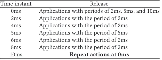
Table 1. An Example OSEK/VDX OS Time Table of Applications Release
Time instant Release
0ms Applications with periods of 2ms, 5ms, and 10ms 2ms Applications with the period of 2ms
4ms Applications with the period of 2ms 5ms Applications with the period of 5ms 6ms Applications with the period of 2ms 8ms Applications with the period of 2ms
10ms Repeat actions at 0ms
whereIis an identity matrix. According to Ackermann’s formula (Ackermann and Utkin1998), the feedback gain used to stabilize the closed-loop system (i.e., to continuously make x[k+1] approachx[k]) is calculated as
K=[0 · · · 0 1]CO−1γc(Ad). (12)
Note that a stable system will havex[k+1]=x[k] andy[k]=Cx[k] in the steady-state. The static
feedforward gainFis used to make the system outputy[k] track the referencer. We letx[k+1]= x[k] andy[k]=Cx[k]=r. Rearranging Equation (9), leads to
F = C 1
d(I−Ad−BdK)−1Bd
. (13)
3.2 Operating System
As a class of real-time OS widely used in the automotive industry, OSEK/VDX OS supports pre-emptive ixed-priority scheduling. That is, priorities are assigned to applications and at any point in time, the task with the highest priority among all active ones is executed.
On OSEK/VDX OS, tasks can be triggered by events (e.g., interrupts) or by time (alarm peri-ods for task activation). The latter scheme is considered in this work, where each application gets released and is allowed to access the processor periodically. There are various periods of release times and each application is assigned one. Diferent applications may have diferent periods. Ev-ery time an application is released, its program gets the chance to be executed, depending on its priority.
A time table containing all the periodic release times within the alleged hyperperiod (i.e., the minimum common multiple of all periods) needs to be conigured. An example with a set of three periods 2ms, 5ms, and 10ms is illustrated in Table 1. The hyperperiod is equal to 10ms and the time table repeats itself every 10ms by reseting the timer. The assigned priority will determine the execution order of applications. A higher priority is typically assigned to the application released with a shorter period (i.e., the rate monotonic scheduling), since this generally results in a more eicient use of the processor. To be computationally eicient in practice, the priority is often not ixed and given to the task with the earliest deadline, which is the dynamic earliest deadline irst (EDF) scheduling (Buttazzo and Gai2006). It is to be noted that the approach proposed in this work is orthogonal to the scheduling policy.
An example with two applicationsC1andC2sharing one ECU is illustrated in Figure4.C1has a
period of 2ms andC2has a period of 5ms. The execution time ofC1is assumed to be 0.7ms and the
execution time ofC2is assumed to be 2ms.C1has a higher priority thanC2. Within a hyperperiod
of 10ms,C1is released at 0ms, 2ms, 4ms, 6ms, 8ms, and 10ms.C2is released at 0ms, 5ms, and 10ms.
It can be seen thatC2is executed only whenC1does not require to access the ECU. For instance,
Fig. 4. Release and execution time of two applications sharing one ECU.C1with a sampling period of 2ms
has a higher priority thanC2with a sampling period of 5ms. Execution times ofC1andC2are 0.7ms and
2ms, respectively.
Fig. 5. Illustration of the controller design with an example scheduleS0={2ms,2ms,2ms,2ms,2ms,5ms,
5ms}. The actuation occurs at the end of a sampling period. The figure is not drawn to scale.
whileC2has to wait. At 0.7ms,C1completes its execution andC2gets the access to the ECU. At
2ms,C1 starts its execution. AlthoughC2 has not completed its execution, it is preempted and
suspended.
Feedback control under OSEK/VDX OS:As can be seen from the above example, in the preemp-tive scheduling of OSEK/VDX OS, the execution completion time of the control program varies in diferent sampling periods. Therefore, we postpone the actuation to the end of a sampling pe-riod, i.e., the to-actuator delay is equal to one sampling pepe-riod, to avoid varying sensor-to-actuator delays. Referring to Equation (8) and as illustrated in Figure5, the control inputu[k] computed based on the system statex[k] sampled at the time instanttk, is applied to the plant at the time instanttk+1.x[k+1] is then dependent on its previous statex[k] and the control input
u[k−1], which is computed based onx[k−1] and applied attk. It is noted that in this work, the control inputu[k] is also dependent on the previous control inputu[k−1], which will be explained later in Section4. The system dynamics in Equation (5) becomes
x[k+1]=Adx[k]+Bdu[k−1]. (14)
Processor Load:We assume that the set of available periods restricted by the OSEK/VDX OS isϕ. As briely discussed in Section1, control applications have to be sampled with one period or a combination of multiple periods fromϕ. In the latter case, switching between two sampling periods can only occur at the common multiplier of them, as has been illustrated in Figure2. Often, the optimal sampling period for a control application does not belong to the setϕ. The simple and straightforward method used in practice is to select the largest sampling period inϕthat is smaller than the optimal one. Taking the example in Table1, assuming that the optimal sampling period is 7.5ms, then 5ms is chosen as the sampling period to be used. This results in a higher processor load, which is an important design aspect.
Denotingeito be the WCET of a control applicationCi, if the uniform sampling period ish, the processor load forCiis
Li = ei
[image:10.486.60.431.185.268.2]The upper bound on the load of any processor is denoted asU. Considering a single processorp,
{i|Ciruns onp}
Li ≤U. (16)
Under the EDF scheduling, the upper boundU is equal to 1. Under the rate monotonic scheduling, U is equal tom(21/m −1), wheremis the number of applications running onp(Liu and Layland 1973). A variety of tools, such as Inchron (2017), Timing Architects (2017), and Symtavision (2017), are used in the industry for more general scheduling analysis. Clearly, increasing the sampling period of a control application decreases its processor load and thus potentially enables more applications to be integrated on the ECU.
4 CONTROLLER WITH NON-UNIFORM SAMPLING
The design problem for a control applicationCi in this work is to reduce the processor loadLi, while satisfying the settling time requirementts0,i, the system stability and the input saturation constraintUmax,i. Towards this, we propose a controller with non-uniform sampling switching among multiple sampling periods inϕ.
The cyclic sequence of sampling periods for a control application deines a scheduleS,
S={T1,T2,T3, . . . ,TN}, (17)
where∀j ∈ {1,2, . . . ,N},Tj ∈ϕ. It implies the sequence of sampling periods as
T1→T2→ · · · →TN →T1→T2→ · · · →TN →repeat
Following the assumption in Equation (15) that the WCET ofCi isei, the processor load forCi overSis
Li =NN ei
j=1Tj
. (18)
Dictated by the scheduleS,Nsystems switch cyclically in a deterministic fashion. The dynamics ofN systems within one cycle ofSis (referring to Equation (14))
x[k+1]=Ad(T1)x[k]+Bd(T1)u[k−1],
x[k+2]=Ad(T2)x[k+1]+Bd(T2)u[k],
.. .
x[k+N]=Ad(TN)x[k+N −1]+Bd(TN)u[k+N −2].
(19)
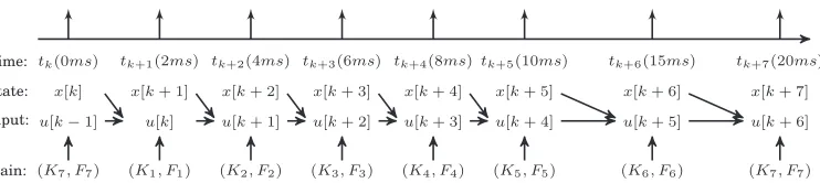
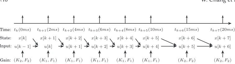
The scheduleS0={2ms,2ms,2ms,2ms,2ms,5ms,5ms}with seven systems is used as an example for the illustration purpose and shown in Figure5. As discussed in Section3.2, the actuation occurs at the end of a sampling period and the sensor-to-actuator delay is equal to one sampling period. For example, the control inputu[k] is computed based on the system statex[k] attkand actuated attk+1.
We introduce a new augmented statez[k]=[x[k]u[k−1] ]T. Then, ∀j∈ {1,2, . . . ,N},
z[k+j]=
A
d(Tj) Bd(Tj)
0 0
z[k+j−1]+
0
1
u[k+j−1], (20)
where0is a zero vector.AauдandBauдare the system matrix and input matrix for the new aug-mented state, and denoted as
Aauд(Tj) =
A
d(Tj)Bd(Tj)
0 0
, Bauд(Tj)=
0
1
The system output is
y[k+j−1]=Cauдz[k+j−1], (22) where
Cauд=[C0 ]. (23)
The control input is designed as
u[k+j−1]=Kjz[k+j−1]+Fjr. (24)
As shown in Figure5, for example,u[k] is computed fromx[k],u[k−1], andK1. Combining
Equa-tions (20), (21), and (24), the closed-loop dynamics is
z[k+j]=Aauд(Tj)z[k+j−1]+Bauд(Tj)u[k+j−1]
=(Aauд(Tj)+Bauд(Tj)Kj)z[k+j−1]+Bauд(Tj)Fjr. (25) We denote the closed-loop system matrix as
Acl,j =Aauд(Tj)+Bauд(Tj)Kj. (26)
It is noted that Equations (22), (24), (21), (25), and (26) are applied for everyjin{1,2, . . . ,N}. In the following of this section, we continue not to repeat the condition.
According to Equation (25), the overall dynamics within a cycle of the exampleS0is
z[k+7]=Acl,7z[k+6]+Bauд(T7=5ms)F7r
=Acl,7(Acl,6z[k+5]+Bauд(T6=5ms)F6r)+Bauд(T7=5ms)F7r
=Acl,7Acl,6z[k+5]+Acl,7Bauд(T6=5ms)F6r +Bauд(T7=5ms)F7r
=Acl,7Acl,6(Acl,5z[k+4]+Bauд(T5=2ms)F5r)
+Acl,7Bauд(T6=5ms)F6r+Bauд(T7=5ms)F7r
=Acl,7Acl,6Acl,5z[k+4]+Acl,7Acl,6Bauд(T5=2ms)F5r
+Acl,7Bauд(T6=5ms)F6r+Bauд(T7=5ms)F7r
.. .
=
7
j=1
Acl,jz[k]+
7
j=2
Acl,jBauд(2ms)F1r+
7
j=3
Acl,jBauд(2ms)F2r
+
7
j=4
Acl,jBauд(2ms)F3r+
7
j=5
Acl,jBauд(2ms)F4r
+
7
j=6
Acl,jBauд(2ms)F5r+Acl,7Bauд(5ms)F6r+Bauд(5ms)F7r.
(27)
If the pair(Aauд(Tj),Bauд(Tj))is controllable, then the feedback gainKj can be designed by pole-placement and computed as per Equation (12),
Kj =[0 · · · 0 1]CO−j1γc(Aauд(Tj)), (28)
where
COj =[Bauд(Tj) Aauд(Tj)Bauд(Tj) · · · Aauд(Tj)n−1Bauд(Tj)]. (29) Poles to place are eigenvalues ofAcl,j. The number of poles is(n+1)N. To ensure stability, eigen-values of the overall closed-loop system matrix7
j=1Acl,j must have absolute values of less than
Fj is computed in a similar way to Equation (13). In Equation (25), we letz[k+j]=z[k+j−1]
andy[k+j−1]=Cauдz[k+j−1]=r. Then we have
z[k+j−1]=(Aauд(Tj)+Bauд(Tj)Kj)z[k+j−1]+Bauд(Tj)FjCauдz[k+j−1]. (30)
This equation is valid, no matter what valuez[k+j−1] takes. Therefore,
I=Aauд(Tj)+Bauд(Tj)Kj+Bauд(Tj)FjCauд. (31)
Then,
Fj = C 1
auд(I−Aauд(Tj)−Bauд(Tj)Kj)−1Bauд(Tj)
. (32)
5 PSO-BASED POLE-PLACEMENT
We now formulate an optimization problem for the pole-placement as
min
D ts
subject to
|u[k]| ≤Umax, ts ≤ts0,
(33)
where poles are decision variables. The settling timets, which can be evaluated with simulation de-pending on the decision variables, is to be minimized as the objective. There are three constraints. First, the input saturation has to be respected. Second, the settling time requirement has to be sat-isied. Third,Dis a domain of poles ensuring the stability of the overall system. We try to optimize
the settling time beyond the requirement, so that the control performance can be maximized while nothing else (e.g., the processor load) needs to be compromised.
It is challenging to solve such a constrained non-convex optimization problem with signiicant non-linearity. We use the eicient PSO technique (Sedighizadeh and Masehian2009). A group of particles are randomly initialized in the decision space with positions and velocities. The particles represent decision variables (i.e., controller poles). They search for the optimum by iteratively updating their positions. The search is led by two points. The irst is the local best point that has been reached by a particle. Every particle has its own local best point. The second is the global best point that has been reached considering all particles. We let feasibility dominate performance when comparing two points:
• A point respecting all constraints is better than a point violating one or more constraints. That is, the objective value has no inluence.
• If both points respect all constraints, then the point with a shorter settling time (i.e., the optimization objective) is considered better.
• If neither of the points respects all constraints (i.e., both of them violate at least one con-straint), then still the point with a shorter settling time is considered better.
The velocity of a particle is determined by the following equation:
Vnew=α0Vcurrent+α1rand(0,1)(Plbest−Pcurrent)+α2rand(0,1)(Pgbest−Pcurrent), (34)
whereVnewis the new velocity,Vcurrentis the current velocity,Pcurrentis the current position,Plbest is the local best point of this particle andPgbestis the best point of all particles. rand(0,1) is a random number with uniform distribution from the open interval(0,1).α0is the weight inertia.
α1andα2are cognitive and social scaling parameters. Widely used values for these parameters are
which have been shown to have good performance in many optimization scenarios. The new position of this particle is
Pnew=Pcurrent+Vnew. (36)
The algorithm is terminated once all particles have converged or the maximum number of itera-tions has been reached. The timing complexity of PSO is clearly polynomial.
ALGORITHM 1:Pole-placement with PSO
Input:PoleNum,ParticleNum,IterationNum Output:Pgbest
1 fori←1toParticleNumdo
2 forj←1toPoleNumdo
3 Randomly initializePi
jin [0,1]
4 Vi
j =0
5 end
6 Pi
lbest=Pi ={P1i,Pi2, . . . ,PPoleNumi }
7 end
8 RecordPgbest 9 k=0
10 whilek<IterationNumandnot all particles have convergeddo 11 UpdateVi
j andPij with (34) and (36)
12 fori←1toParticleNumdo
13 UpdatePilbest 14 end
15 UpdatePgbest 16 k=k+1 17 end
The pseudocode is shown in Algorithm1to illustrate the pole-placement with PSO. Every pole of every particle is randomly initialized in [0,1] (Line 3). This gives the initilized particles a good chance of being feasible (i.e., satisfying all the constraints). The velocity is initialized to be 0 (Line 4). The local best point of every particle (Line 6) and the global best point of all particles (Line 8) are recorded. Afterwards, we iteratively update the position and velocity of every particle (Line 11). At every iteration, we record the local best point of each particle (Line 13) and the global best point of all particles (Line 15). Once the algorithm is terminated, the global best point is re-turned. It is noted that we do not impose hard feasibility requirement in this algorithm. The rules that prioritize feasibility over performance when comparing two points drive the search towards the feasible region. The inal solution has the best performance among all the visited feasible points during the search.
One major issue with PSO is its tendency for fast and premature convergence before the global optimum has been found, since its search is highly directional (Sedighizadeh and Masehian2009). This problem gets more severe as the number of dimensions in the decision space grows larger. The cognitive and social scaling parametersα1 andα2 have a signiicant impact on the search
behavior and convergence of PSO. Ifα1is larger thanα2, then the PSO tends to have better local
searches, yet converges more slowly. Ifα2 is larger thanα1, then the PSO often converges fast
There have been a number of works extensively investigating the parameterization of PSO (Jordehi and Jasni 2013; Pedersen 2010; Nickabadi et al.2011). Various existing strategies for PSO parameters setting are summarized in Jordehi and Jasni (2013), which discusses some fu-ture research directions. A list of good parameter choices for several benchmarks is reported in Pedersen (2010). An adaptive inertia weight is proposed in Nickabadi et al. (2011) and uses the suc-cess rate of the swarm as its feedback parameter to ascertain the particles’ situation in the search space. In this work, we propose an adaptive parameterization approach for the cognitive and social scaling parameters with a constant sum. As the iteration number increases,α1 is decreased and
α2increases. The basic idea is that at the beginning of the optimization when particles are more
disperse, local areas are better searched aiming to explore a larger space. When the optimization approaches to the end, particles are close to one another, and the focus is placed on convergence. The goal is to achieve optimality and eiciency at the same time.
Assuming that the iteration number isq(0<q ≤qmax, whereqmax is the maximum number of iterations), the cognitive and social scaling parameters can be computed as
α2=f
q qmax
, α1=4−α2, (37)
where the constant sum ofα1andα2is taken as 4.f is a function that can be customarily decided.
In this work, we use an exponential function as
f(x) =0.5e2x+0.1. (38)
A numerical example is used to show the advantage of the proposed adaptively parameterized PSO technique. The formulation is as follows:
max
D φ=e
−13β13+β1−β22
subject to
D={(β1,β2)| −1.8≤β1 ≤2, −2≤β2≤2},
(39)
whereβ1andβ2are two continuous decision variables, constrained in the decision spaceD. The
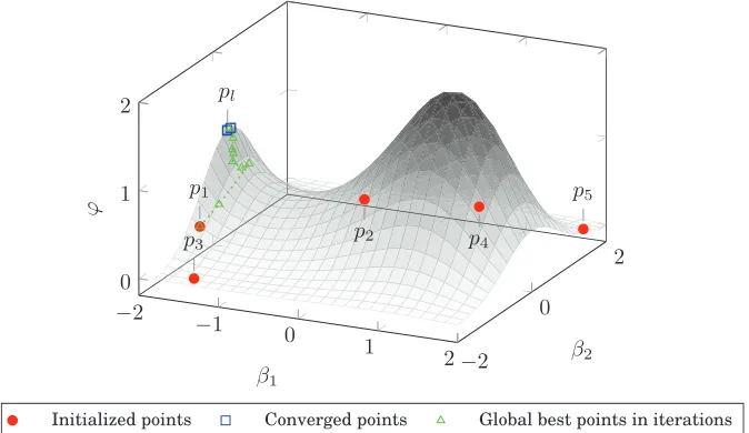
objective to maximize isφ. The conventional PSO method is illustrated in Figure6. Five parti-cles are randomly initialized atp1,p2,p3,p4, andp5, as shown in Table2. Among them,p1has
the best objective value. After 13 iterations, all ive particles converge to points around the local optimumpl (β1=−1.7997,β2=8.3188×10⁻³,φ=1.1540). The path showing how the global best
point evolves iteratively is drawn, with certain points that are too close to others omitted for better illustration. It can be seen that the search is highly directed towards the global best point in each iteration. The global optimum is not found and particles quickly converge to the local optimum before exploring the decision space suiciently.
The proposed novel PSO method with adaptive parameterization is illustrated in Figure7. The same initial points are used as in Figure6and Table2. After 13 iterations, all ive particles converge to points around the global optimumpд(β1=9.8765×10⁻¹,β
2=−3.9853×10⁻³,φ
Fig. 6. With the conventional particle swarm optimization method, five particles are randomly initilized and converge to the local optimumpl.
Table 2. Randomly Initialized Particles in the Numerical Example of PSO
Particle p1 p2 p3 p4 p5
β1 −1.7 −0.8 −1.4 0.5 1.9
β2 −1 1.5 −1.8 1.8 1.6
φ 0.3456 0.0562 0.0241 0.0619 0.0525
Fig. 8. Illustration of the alternative more scalable controller design with an example scheduleS0. Gains are the same for systems with the same sampling period. The figure is not drawn to scale.
6 ALTERNATIVE CONTROLLER DESIGN FOR SCALABILITY
As discussed before, the number of dimensions in the decision space using the controller design presented in Section4is(n+1)N. When the number of sampling periodsN in a schedule is very
large, solving the pole-placement optimization problem could be computationally too heavy, even for an oline task. The PSO-based technique naturally ofers a solution—decreasing the number of particles and iterations. However, this renders the result stochastic with a large variation and considerably dependent on the choices during initialization, which is often undesirable. In this section, we provide an alternative controller design aiming for better scalability on the number of sampling periods.
The complexity of the proposed controller in Section 4comes from that the closed-loop dy-namics of all the sampling periods are considered and optimized. A simpler design technique is to assume identical closed-loop dynamics for the systems with the same sampling period (the same open-loop dynamics as well). That is, ifTj =Tj′, the poles and feedback/feedforward gains
of these two systems are the same. TakingS0 as an example, as shown in Figure8, for the ive systems with the sampling period of 2ms, poles are assumed to be the same. Therefore, the feedback gains are all K1 and the feedforward gains are all F1. The closed-loop system matrix
Aauд(2ms)+Bauд(2ms)K1is considered in the pole-placement. Similarly, for the two systems with
the sampling period of 5ms, feedback gains areK2and feedforward gains areF2. The closed-loop system matrixAauд(5ms)+Bauд(5ms)K2is considered in the pole-placement. Everything else re-mains unchanged with respect to the design described in Section4and Section5.
Clearly, the solution is suboptimal, since the assumption that poles are identical for systems with the same sampling period does not necessarily hold. The advantage is a smaller decision space. The number of decision variables (i.e., poles to place) becomes (n+1)N′—the number of
states of the plant multiplied by the number of distinctive sampling periods in the schedule. For the example scheduleS0,N′is 2 and thus the number of dimensions in the decision space is 27 of the one in Section4. Therefore, when the number of sampling periodsN in the scheduleSis very large and the number of distinctive sampling periodsN′is relatively small, this alternative
controller has better scalability on the number of sampling periods.
7 EXPERIMENTAL RESULTS
Fig. 9. A simplified model of the electro-mechanical braking system.
Table 3. EMB System Requirements
Settling time requirement Input saturation Reference position WCET
150ms 12V 2mm 0.7ms
Table 4. Setling Time and Processor Load of Three Schedules
Schedule Settling time Requirement satisfaction Processor load
S1={5ms} 256.40ms Violated 14%
S2={2ms} 113.27ms Satisied 35%
S0(novel PSO) 132.14ms Satisied 24.5%
S0(conventional PSO) 154.05ms Violated 24.5%
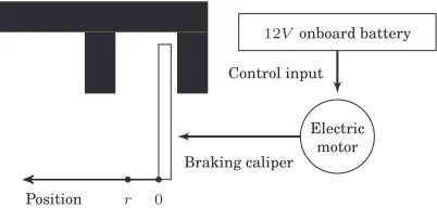
of the EMB system, which is of interest in several scenarios: braking, disk wiping, and pre-crash preparations. The system dynamics can be modeled as
A= ⎡⎢ ⎢⎢ ⎢⎢ ⎢⎢ ⎢⎢ ⎢⎣
−520−220 0 0 0
220 −500−999994 0 2×10⁸
0 1 0 0 0
0 0 66667 −0.1667−1.3333×10⁷
0 0 0 1 0
⎤⎥ ⎥⎥ ⎥⎥ ⎥⎥ ⎥⎥ ⎥⎦
, B=
⎡⎢ ⎢⎢ ⎢⎢ ⎢⎢ ⎢⎢ ⎢⎣ 1000 0 0 0 0 ⎤⎥ ⎥⎥ ⎥⎥ ⎥⎥ ⎥⎥ ⎥⎦ ,
C=0 0 0 0 1.
(40)
There are ive system states—motor current, motor angular velocity, motor angular position, caliper velocity, and caliper position. The control input is the applied voltage on the motor. The re-quirements are summarized in Table3. The set of available sampling periods ofered by OSEK/VDX OS is
ϕ={1ms,2ms,5ms,10ms,20ms,50ms,100ms,200ms,500ms,1s}. (41) In the experiments of this work, we consider the EDF scheduling under the OSEK/VDX OS. When the deadlines are the same, the application with a smaller index has a higher priority.
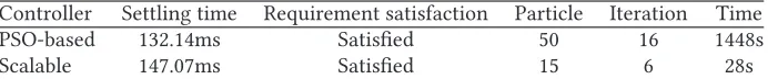
PSO-based controller design with non-uniform sampling:As shown in Table4and Figure10, the scheduleS1={5ms}cannot meet the settling time requirement. The largest sampling period
smaller than 5ms inϕis 2ms. The scheduleS2={2ms}is able to fulill all the requirements.
Ac-cording to Equation (15), using the WCET requirement in Table3, the processor load ofS2 is 35%. As discussed before, this number can be unnecessarily large and prevents more applications from sharing the ECU.
Then we evaluate the schedule S0={2ms,2ms,2ms,2ms,2ms,5ms,5ms} switching between
[image:18.486.107.384.385.463.2]Fig. 10. System output of three diferent schedules. The proposed PSO technique is used forS0.
Fig. 11. System output of the PSO-based controller and its scalable variant.
Table 5. Comparison of the PSO-based Controller Design with Its Scalable Variant
Controller Settling time Requirement satisfaction Particle Iteration Time
PSO-based 132.14ms Satisied 50 16 1448s
Scalable 147.07ms Satisied 15 6 28s
discussed in Section3.2. The controller with non-uniform sampling is designed as proposed in Sec-tion4and the novel PSO with adaptive parameterization as in Section5is used for pole-placement. 50 particles are deployed and converge after 16 iterations. Increasing the number of particles be-yond 50 does not further improve the control performance. There are 42 poles from the seven closed-loop system matrices. S0 has a slightly longer settling time thanS2, yet still fulills the requirement. According to Equation (18), the processor load is 24.5%, achieving a 30% reduction compared toS2. We also evaluate the settling time ofS0 using the conventional PSO technique. Fifty particles are used, and the convergence also takes 16 iterations. As reported in Table4, the solution does not satisfy the requirement.
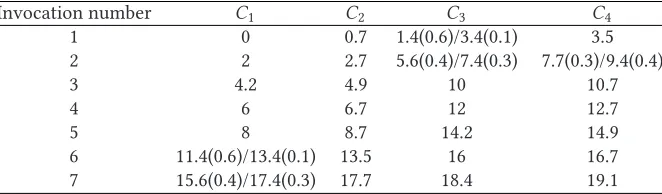
[image:19.486.71.417.444.480.2]Fig. 12. Invocation timing of four control applications under the scheduleS0. The schedule forC1andC2is
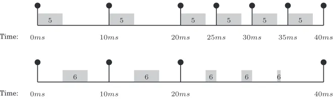
{2ms,2ms,2ms,2ms,2ms,5ms,5ms}, and the schedule forC3andC4is{5ms,5ms,2ms,2ms,2ms,2ms,2ms}. Numbers 1, 2, 3, and 4 represent the applicationsC1,C2,C3, andC4, respectively. Preemption is allowed in
OSEK/VDX OS.
Table 6. Exact Invocation Starting Times of Four Control Applications Under the Non-uniform Sampling ScheduleS0
Invocation number C1 C2 C3 C4
1 0 0.7 1.4(0.6)/3.4(0.1) 3.5
2 2 2.7 5.6(0.4)/7.4(0.3) 7.7(0.3)/9.4(0.4)
3 4.2 4.9 10 10.7
4 6 6.7 12 12.7
5 8 8.7 14.2 14.9
6 11.4(0.6)/13.4(0.1) 13.5 16 16.7
7 15.6(0.4)/17.4(0.3) 17.7 18.4 19.1
When one invocation is preempted, two starting times are separated by a forward slash, and the number in the bracket indicates the duration. The timing unit is ms.
by the scalable controller is longer, yet still satisies the requirement. It takes 15 particles that con-verge after 6 iterations. Increasing the number of particles beyond 15 does not further improve the control performance. The total computation time on a computer with an Intel i5 processor oper-ating at 2.6GHz with 4GB RAM is 28s, compared to 1448s for the controller aiming for optimality. Although 1448s sounds acceptable for an oline task, when a schedule has more sampling periods thanS0, the computation could take hours or even days due to the increase of the decision space dimensions. In such a case, if the number of distinctive sampling periods is small, the scalable controller design is preferred.
Packing of more applications:Now we consider a case that multiple applications are to be im-plemented on ECUs. For the convenience of illustration, all applications are assumed to be identi-cal to the EMB system discussed before with the WCET of 0.7ms. As reported above, the schedule S2={2ms}is able to satisfy the control performance requirement and system constraints. Under
S2, an ECU is able to accommodate two applications according to Equation (16). Under the non-uniform sampling scheduleS0, four applications can share one ECU, where detailed invocation timing is presented in Figure12and Table6. Numbers 1, 2, 3, and 4 represent the applicationsC1,C2,
C3, andC4, respectively. While the schedule forC1andC2is{2ms,2ms,2ms,2ms,2ms,5ms,5ms},
the schedule forC3andC4is{5ms,5ms,2ms,2ms,2ms,2ms,2ms}. The switching of sampling
[image:20.486.78.409.270.367.2]Fig. 13. Invocation timing ofC5andC6under the non-uniform sampling schedules. The schedule forC5is
{10ms,10ms,5ms,5ms,5ms,5ms}, and the schedule forC6is{10ms,10ms,20ms}. Numbers 5 and 6 represent
the applicationsC5andC6, respectively.
Table 7. Exact Invocation Starting Times ofC5andC6under the Non-uniform
Sampling Schedules
Invocation number 1 2 3 4 5 6
C5 0 10 20 25 30 35
C6 3.5 13.5 23.5(1.5)/28.5(1.5)/33.5(0.5) N.A. N.A. N.A.
When one invocation is preempted, two starting times are separated by a forward slash and the number in the bracket indicates the duration. The timing unit is ms.
ECU, others are in the longer sampling period (5ms in this case), requesting the execution less often. In this way, the number of applications packed onto the ECU can be maximized.
It is noted that preemption is supported in OSEK/VDX OS. In this case, we consider the EDF scheduling. For instance, at 1.4ms when bothC1andC2inish their irst invocations,C3is started
and allowed to access the processor for 0.6ms. After that,C3is suspended, waiting for the second
invocations ofC1andC2, which have higher priorities. Then,C3resumes and completes its irst
invocation.
It can be seen that the number of applications that are accommodated by an ECU is doubled with the proposed OS-aware non-uniform sampling controller design, which is signiicant improvement for the cost-sensitive automotive domain.
To further validate the advantages brought by the proposed approach, we consider another case consisting of applications with diferent non-uniform sampling schedules. We assume that the schedule with the uniform sampling period 5ms is able to satisfy the performance require-ment of the applicationC5. We also assume that the non-uniform sampling schedule with two
sampling periods 5ms and 10ms satisies the performance requirement ofC5. However, the
sched-ule with the uniform sampling period 10ms does not satisfy the performance requirement ofC5.
The performance requirement of the applicationC6can be satisied with the schedule{10ms}and
{10ms,10ms,20ms}, yet not {20ms}. The WCETs of bothC5C6 are 3.5ms. If only uniform
sam-pling schedules are considered, thenC5 andC6 cannot be implemented on one processor, since
the total processor load is 3.5/5+3.5/10=1.05, which exceeds the upper bound 1 as discussed in Equation (16). If non-uniform sampling schedules are deployed, then bothC5andC6can be
imple-mented on one processor. Detailed invocation timing is presented in Figure13and Table7. It can be seen that the processor can run another strictly periodic application. If the period is 5ms, then the longest allowed WCET is 0.625ms. It is noted that the third invocation ofC6 will be evenly
8 CONCLUDING REMARKS
To deal with the restriction imposed by the OS on sampling periods for control applications, we present a novel performance-oriented controller design with a non-uniform sampling schedule, in which an adaptively parameterized PSO is used for pole-placement. It reduces the processor load, while satisfying the control performance requirement and system constraints. This saves computation resources and enables integration of more functions and applications into an ECU, thereby saving costs, which is critical in the automotive domain. Experimental results show that the number of control applications sharing an ECU can be higher with the proposed OS-aware controller design with non-uniform sampling.
The focus of this article is to show that more applications can be packed using a non-uniform sampling schedule and the proposed controller design method. A relevant question for the future works is the design of the optimal sampling schedule. Given that the controller design has to be redone for every possible schedule, the optimal schedule design is a non-trivial problem, especially when the number of applications sharing one processor is large. However, by checking the per-formance of uniform sampling schedules (e.g., the period of 2ms is able to satisfy the perper-formance requirement and the period of 5ms is not), it is possible to intuitively come up with a few non-uniform sampling schedules as candidates of design interest (e.g., schedules switching between 2ms and 5ms, 1ms, and 10ms, etc.) to be evaluated with the approach proposed in this article.
While in this article the focus was on single-core ECUs, we intend to extend our approach to multi-core architectures. There are mainly two challenges to address. First, due to load balancing requirements, it might be necessary to distribute diferent parts of complex control applications to diferent cores. This introduces additional delays for sensor-to-actuator cause-efect chains that need to be taken into account during controller design to ensure stability. Second, memory par-titioning and code placement need to be considered, since they have a major inluence on the execution times of control programs.
REFERENCES
2017. Inchron GmbH. Retrieved fromhttps://www.inchron.de/.
2017. Symtavision GmbH. Retrieved fromhttps://www.symtavision.com/. 2017. Timing Architects. Retrieved fromhttp://www.timing-architects.com/.
Juergen Ackermann and Vadim Utkin. 1998. Sliding mode control design based on Ackermann’s formula.IEEE Trans. Au-tomat. Control43, 2 (1998), 234–237.
Adolfo Anta and Paulo Tabuada. 2009. On the beneits of relaxing the periodicity assumption for networked control systems over CAN. InProceedings of the 30th IEEE Real-Time Systems Symposium (RTSS’09).
Vincenzo Apuzzo, Alessandro Biondi, and Giorgio C. Buttazzo. 2016. OSEK-like kernel support for engine control appli-cations under EDF scheduling. InProceedings of the 22nd IEEE Real-Time and Embedded Technology and Applications Symposium (RTAS’16).
Karl J. Åström and Richard M. Murray. 2009.Feedback Systems: An Introduction for Scientists and Engineers. Princeton University Press.
Enrico Bini and Giuseppe M. Buttazzo. 2014. The optimal sampling pattern for linear control systems.IEEE Trans. Automat. Control59, 1 (2014), 78–90.
Giorgio Buttazzo and Paolo Gai. 2006. Eicient EDF implementation for small embedded systems. InProceedings of the 2006 International Workshop on Operating Systems Platforms for Embedded Real-Time Applications (OSPERT’06).
Rosa Castane, Pau Marti, Manel Velasco, Anton Cervin, and Dan Henriksson. 2006. Resource management for control tasks based on the transient dynamics of closed-loop systems. InProceedings of the 18th. Euromicro Conference on Real-Time Systems (ECRTS’06).
Anton Cervin, Johan Eker, Bo Bernhardsson, and Karl-Erik Årzén. 2002. Feedback-feedforward scheduling of control tasks. Real-Time Syst.23, 1–2 (2002), 25–53.
Anton Cervin, Manel Velasco, Pau Marti, and Antonio Camacho. 2011. Optimal online sampling period assignment: Theory and experiments.IEEE Trans. Control Syst. Technol.19, 4 (2011), 902–910.
OSEK/VDX Consortium. 2005. OSEK/VDX operating system speciication Version 2.2.3.
Peter H. Feiler. 2003.Real-time Application Development with OSEK: A Review of the OSEK Standards. Technical Report. Carnegie Mellon University.
Luca Greco, Daniele Fontanelli, and Antonio Bicchi. 2011. Design and stability analysis for anytime control via stochastic scheduling.IEEE Trans. Automat. Control56, 3 (2011), 571–585.
Shengyan Hong, Xiaobo Sharon Hu, Tao Gong, and Song Han. 2015. On-line data link layer scheduling in wireless net-worked control systems. InProceedings of the 27th Euromicro Conference on Real-Time Systems (ECRTS’15).
Shengyan Hong, Xiaobo Sharon Hu, and Michael Lemmon. 2010. Reducing delay jitter of real-time control tasks through adaptive deadline adjustments. InProceedings of the 22nd Euromicro Conference on Real-Time Systems (ECRTS’10). Kyusoo Jeong, Donggon Lee, Sungwook Park, and Changsik Lee. 2011. Efect of two-stage fuel injection parameters on
NOx reduction characteristics in a DI diesel engine.Energies4, 11 (2011), 2049–2060.
Ahmad Rezaee Jordehi and Jasronita Jasni. 2013. Parameter selection in particle swarm optimization: A survey.J. Exp. Theor. Artif. Intell.25, 4 (2013), 527–542.
Simon Kramer, Dirk Ziegenbein, and Arne Hamann. 2015. Real world automotive benchmark for free. InProceedings of the 6th International Workshop on Analysis Tools and Methodologies for Embedded and Real-Time Systems (WATERS’15). Eugene Lavretsky and Kevin Wise. 2013.Robust and Adaptive Control with Aerospace Applications. Springer.
Michael Lemmon and Xiaobo Sharon Hu. 2011. Almost sure stability of networked control systems under exponentially bounded bursts of dropouts. InProceedings of the 14th. ACM International Conference on Hybrid Systems: Computation and Control (HSCC’11).
Hai Lin and Panos J. Antsaklis. 2009. Stability and stabilizability of switched linear systems: A survey of recent results. IEEE Trans. Automat. Control54, 2 (2009), 308–322.
Chunglaung Liu and James W. Layland. 1973. Scheduling algorithms for multiprogramming in a hard-real-time environ-ment.J. ACM20, 1 (1973), 46–61.
Ahmad Nickabadi, Mohammad Mehdi Ebadzadeh, and Reza Safabakhsh. 2011. A novel particle swarm optimization algo-rithm with adaptive inertia weight.Appl. Soft Comput.11, 4 (2011), 3658–3670.
Magnus Erik Hvass Pedersen. 2010.Good Parameters for Particle Swarm Optimization. Technical Report. Hvass Laboratories. Dobrivoje Popovic, Mrdjan Jankovic, Steve Magner, and A. Teel. 2003. Extremum seeking methods for optimization of
variable cam timing engine operation. InProceedings of the 2003 American Control Conference (ACC’03). James B. Rawlings and David Q. Mayne. 2009.Model Predictive Control: Theory and Design. Nob Hill Publishing. Debayan Roy, Licong Zhang, Wanli Chang, Dip Goswami, and Samarjit Chakraborty. 2016. Multi-objective co-optimization
of lexray-based distributed control systems. InProceedings of the 22nd IEEE Real-Time and Embedded Technology and Applications Symposium (RTAS’16).
Davoud Sedighizadeh and Ellips Masehian. 2009. Particle swarm optimization methods, taxonomy and applications.Int. J. Comput. Theory Eng.1, 4 (2009), 486–502.
Dong Yue, Engang Tian, and Qinglong Han. 2013. A delay system method for designing event-triggered controllers of networked control systems.IEEE Trans. Automat. Control58, 2 (Feb. 2013), 475–481.