Exploiting lattice structures in shape grammar implementations

and Manufacturing

cambridge.org/aie

Research Paper

Cite this article:Chau HH, McKay A, Earl CF, Behera AK, de Pennington A (2018). Exploiting lattice structures in shape grammar implementations.Artificial Intelligence for Engineering Design, Analysis and Manufacturing 32, 147–161. https://doi.org/10.1017/ S0890060417000282

Received: 15 October 2016 Revised: 17 May 2017 Accepted: 17 May 2017 Key words:

Ambiguity; bill of materials (BOM) structures; complemented distributive lattice; design descriptions; maximal representation; set grammars; shape emergence

Author for correspondence:

Hau Hing Chau, E-mail:H.H.Chau@leeds.ac.uk

© Cambridge University Press 2018. This is an Open Access article, distributed under the terms of the Creative Commons Attribution licence (http://creativecommons.org/licenses/ by/4.0/), which permits unrestricted re-use, distribution, and reproduction in any medium, provided the original work is properly cited.

grammar implementations

Hau Hing Chau1_{, Alison McKay}1_{, Christopher F. Earl}2_{, Amar Kumar Behera}1 and Alan de Pennington1

1

School of Mechanical Engineering, University of Leeds, Leeds LS2 9JT, UK and2School of Engineering and Innovation, The Open University, Milton Keynes MK7 6AA, UK

Abstract

The ability to work with ambiguity and compute new designs based on both defined and emergent shapes are unique advantages of shape grammars. Realizing these benefits in design practice requires the implementation of general purpose shape grammar interpreters that sup-port: (a) the detection of arbitrary subshapes in arbitrary shapes and (b) the application of shape rules that use these subshapes to create new shapes. The complexity of currently avail-able interpreters results from their combination of shape computation (for subshape detection and the application of rules) with computational geometry (for the geometric operations need to generate new shapes). This paper proposes a shape grammar implementation method for three-dimensional circular arcs represented as rational quadratic Bézier curves based on lattice theory that reduces this complexity by separating steps in a shape computation process from the geometrical operations associated with specific grammars and shapes. The method is dem-onstrated through application to two well-known shape grammars: Stiny’s triangles grammar and Jowers and Earl’s trefoil grammar. A prototype computer implementation of an inter-preter kernel has been built and its application to both grammars is presented. The use of Bézier curves in three dimensions opens the possibility to extend shape grammar implemen-tations to cover the wider range of applications that are needed before practical implementa-tions for use in real life product design and development processes become feasible.

Introduction

Shape grammars have been used successfully to explore design spaces in various design con-texts (Strobbe et al.,2015). They are used to both analyze existing styles and generate new designs. Generative capability and shape emergence are two aspects of shape grammars that make them appealing to designers, and many implementations have illustrated how designers might take advantage of this generative capability (Chase,2010). However, there is a range of shape emergence capabilities in these implementations and shape emergence is generally restricted, in each implementation, to particular kinds of shape. This paper demonstrates the potential of lattice structures to improve the shape emergence capabilities ofU13 shape grammar implementations. Shape emergence algorithms in current implementations are com-plex, in part, because computational geometry and shape computation are considered simul-taneously. This paper provides a mechanism where lattices are used to reduce this complexity by decoupling computational geometry (needed for the geometrical operations associated with specific grammars used in the generation of new shapes) and shape computation (needed for sub-shape detection and the application of rules). A prototype implementation of an inter-preter kernel has been built and applied to two well-known shape grammars: Stiny’s triangles grammar (Stiny,1994) and Jowers and Earl’s trefoil grammar (Jowers & Earl, 2010). Early results are promising with more applications, for wider evaluation, and integration with suitable user interfaces as important next steps.

Background and related works

Existing shape grammar implementations that support emergence

Computer implementation of shape grammars with shape emergence is challenging (Chase,

The goal of this research is to provide a shape grammar imple-mentation method that is extensible to a wide range of curves (any that can be represented as a rational Bézier curve) and dimensionalities. Such implementations are needed if shape grammars are to be used as generative design tools in product development processes. For this reason, implementations that support emergence in parametric grammars using rectilinear shapes, for example, Grasl and Economou (2013) are not included. Other implementations that allow emergence, such as those based on bitmap representations (Jowers et al.,2010), are not included because they represent shapes using discrete pixels, essentiallyU02which, again, limits their extensibility.

Shape grammar interpreter (Krishnamurti,1981), uses straight lines as basic elements, but lines parallel with they-axis are trea-ted differently to lines that are not. Chase (1989) reports further progress on the consideration of automatic subshape recognition of shapes consisting of straight lines in any orientation and GEdit (Tapia, 1999) presents users with a visualization of choices of how shape rules based on straight lines can be applied. Shape grammar synthesizer (Chau et al., 2004; Li et al., 2009) uses straight line segments and circular arcs in three dimensions and Jowers and Earl (2011) used quadratic Bézier curve segments as basic elements in two dimensions. Each of these implementations considers computational geometry and shape computation simul-taneously with special cases used to cater for the different geometric combinations in the shape computation process. As a result, extending any of these [five] implementations to cover more shapes and/or dimensionalities would be challenging because of the growth in the number of special cases needed, which is in the order of ann2problem. The approach proposed in this paper explores the potential of lattice structures to decou-ple steps in a shape computation from the geometrical operations associated with specific grammars. This removes the need for the treatment of special cases and so makes the method more exten-sible because it transforms it into the order of annproblem. A fuller description of the proposed approach and a detailed com-parison with Jowers and Earl’s method are included in later sec-tions of this paper.

In the 1999 NSF/MIT Workshop on Shape Computation, one of the four sessions was devoted to computer implementations of shape grammars (Gips, 1999). One discussion area considered whether a single implementation could support both shape emergence and parametric grammars. It was acknowledged that significant research challenges needed to be resolved before both could be achieved. Nearly two decades later, we can find the most substantial grammars, especially in architectural design, are parametric and can be used to both describe styles and gener-ate new designs. On the other hand, Grasl and Economou (2013)

made significant headway to support shape emergence in para-metric grammars using straight lines.

Graph grammar implementations for spatial grammars

Graph grammars are a popular approach for the analysis of styles in architectural and other kinds of design (Rudolph,2006; Grasl,

2012). Grasl and Economou (2013) used graphs and a meta-level abstraction in the form of a hypergraph. Graph grammars also offer tractable implementations of shape grammars, in that they make use of established algorithms for graph operations and rules. The graphs describe shapes in terms of the incidence of shape elements. A range of incidence structures are used in imple-mentations. Each depends on the underlying parts chosen to represent a shape. These range from elements corresponding to the polygons of edges in the shape to incidence between line ele-ments. Substructures in these incidence structures can correspond to emergent shapes. Graph type incidence structures represent binary relations among elements. Higher dimensional relations, where several elements may be mutually related, can be repre-sented by hypergraphs (Berge, 1973). This correspondence is used to good effect by Grasl and Economou (2013) in their appli-cation of graphs and hypergraphs to enable shape emergence in straight line shapes inU13. The graph grammar implementations allow recognition of substructures which may correspond to emergent shapes.

Terminology and the application of lattice theory

The approach proposed in this paper is used for each rule appli-cation in a given shape computation process where the rule is applied under affine transformations except shears. For this rea-son, there are two inputs: a shape rule and an initial shape. Lattice structures are used because of their ability to represent all possible combinations of the collection of shape elements that form the initial shape and could result from the application of the rule. Each node in the lattice represents either a shape ele-ment that is a maximal shape (and so not divisible in the shape computation step) or an aggregation of such elements including both sub-shapes that are parts of the initial shape description and emergent shapes.

Terminology

A partially ordered set (poset) has a binary ordering relation that is reflexive, anti-symmetric, and transitive conditions. The binary relation≤can be read as “is contained in”, “is a part of,” or “is less than or equal to” according to its particular application (Szász, 1963). When Hasse diagrams (Figs. 8, 12) are used to Table 1.Basic elements of selected shape grammar implementations that support emergence

Name

Shape grammar interpreter (Krishnamurti,1981)

A Prolog implementation (Chase,1989)

GEdit (Tapia,

1999)

Shape grammar synthesizer (Chau et al.,2004; Li et al.,

2009)

Quad interpreter (Jowers & Earl,2010)

Basic element type(s)

Straight lines (non-vertical and vertical lines have different descriptions)

Straight lines in 2D Straight lines in 2D

Straight lines in 3D and limited support of circular arc

Quadratic Bézier curve in 2D

Descriptors Endpoints Endpoints Endpoints Endpoints and control polygons

Control polygons

Parametric variable range

represent posets, the ordering relation is represented by a line adjoining two nodes that have different vertical positions, where the lower node is a part of the upper one. Their horizontal posi-tions are immaterial. Visual representaposi-tions of lattices, in the form of Hasse diagrams are used in this paper to illustrate how the use of lattices can decouple computational geometry and shape computation aspects. Hasse diagrams are not required in actual use where it is sufficient to store and relate all elements of a lattice symbolically.

A lattice, in our case, is a poset of shapes. Each node is a shape in algebra Uij, which is a subshape of the initial shape for the

given rule and has a set of basic elements (Stiny, 1991). Each

basic element is a shape in its maximal representation (Krishnamurti,1992) and can be divided into its relatively max-imal parts. These relatively maxmax-imal parts are a segmentation of non-overlapping parts based on the element’s intersections with other basic elements in the initial shape. Any tworelatively max-imal partsof a basic element have no common parts. However, these relatively maximal parts are not in maximal representation and can be recombined to form the original basic element.

Lattice theory

Ganter and Wille (1999) use lattices as a basis for formal concept analysis which enables the definition of ontologies (Simons,1987) induced on sets of objects through their attributes. Numerous applications are reported in the literature especially in the Concept Lattice and Their Applications conference series (Ben Yahia & Konecny, 2015; Huchard & Kuznetsov, 2016) which ranges across architecture, engineering and healthcare, and in

The Shape of Things workshop series (Rovetto, 2011;

Ruiz-Montiel et al., 2011). Aggregations of objects in a formal concept lattice [an ontology] allow parts of the aggregation, the objects, to be recategorized using their attributes. For example, cats, dogs, and snails may be the objects that are initially grouped as family pets; defining them in a formal concept lattice could allow them to be recategorized as mammals and mollusks for a different purpose. In this paper, we use lattices in a different way: to provide a symbolic representation of an initial shape in the context of a shape rule in terms of their common parts. The use of lattices in shape applications is less common but there are examples in the literature. For example, March (1983,

1996) used lattices to describe geometric shapes, Stiny (1994,

2006) used a lattice of parts to describe continuity in a sequence of shape rule applications and Krstic (2010,2016) used lattices in shape decompositions.

A lattice (Szász,1963; Grätzer,1971) is a poset such that the least upper bound and the greatest lower bound are unique for any pair of nodes. As a result, for any pair of shapes (represented as nodes) in the lattice, there exists a unique least upper bound

and a unique greatest lower bound. This property is exploited in the detail of the implementation when calculating, for a given shape, its parents, children, and siblings. A lattice satisfies idempotent, commutative, associative, and absorption laws and is one of the fundamental abstract algebra constructs. In this paper, the nodes in a lattice are used to represent shapes in alge-bra U13, and the binary ordering relation≤is the subshape rela-tion. In essence, we use the lattice to create a temporary set grammar based on the initial shape and the rule that is to be applied.

The lattices we use are complemented distributive lattices because, for any complemented lattice, the complement of any node always exists and is unique, and for any distributive lattice, the join of any two nodes always exists and is unique. A comple-mented distributive lattice is a Boolean algebra and these proper-ties allow shape difference and sum operations to be defined in terms of complements and joins. We exploit this as a basis for set grammar computation of the initial shape and the shape rule represented by the lattice.

Proposed method

The crux of the proposed method is to reduce a shape grammar to a set grammar for each application of a rule,A→B, by decom-posing an initial shape, C, into a finite number of shape atoms in the context of the left-hand side of the rule, A. Each atom is a combination of relatively maximal [shape] parts of C. Since shapeChas a finite number of atoms, a corresponding temporary set grammar can be used to compute the shape difference opera-tions needed to calculate the complementsC−t(A) symbolically without considering the actual geometry of eitherCorA. For any given lattice node that is at(A), its complementC−t(A) can be derived from the lattice.

For the purpose of describing one step of a shape computation, which involves the application of a shape grammar rule, a tem-porary set grammar (represented as a lattice) is derived from the rule and the initial shape. This set grammar is only valid for one step of a shape computation. [Shape] atoms, which consist of a number of relatively maximal parts, are nodes in the lattice. A node represents a shape which is composed of atoms. An atom is a non-decomposable shape during this step of the shape compu-tation. All possible matching t(A) and their complements C− t(A) are also nodes in the lattice.

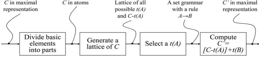
A four-step process (Fig. 1) is proposed for applying a shape rule which may have many potential applications to the initial shape. Aspects of computational geometry and shape computa-tion are decoupled. The computacomputa-tional geometry of basic ele-ments is used in steps 1 and 4, and shape computation in the second and the third. Steps 2 and 3 use the shape algebra of

the set grammar represented by the lattice without considering actual geometry. This is possible because atoms of the set gram-mar are relatively maximal to one another.

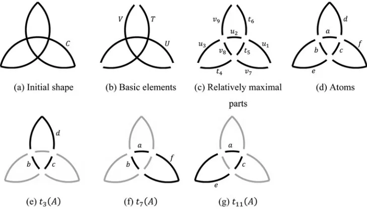
Step 1: divide basic elements into parts

First, basic elements (Fig. 2b) of an initial shapeC (Fig. 2a) are divided into relatively maximal parts (Fig. 2c) under transforma-tions using their registration points (Krishnamurti & Earl,1992). These parts are regrouped to form atoms (Fig. 2d). These atoms of

C are indivisible during an application of a shape rule A→B

under any valid transformationt(Fig. 2e–g). The left-hand side

Aof the rule determines the decomposition ofC.

Registration points are endpoints, control vertices, and intersection points of basic elements of shapes A and C. Three non-collinear registration points from each shape determine a three-dimensional (3D) local coordinate frame that consists of an origin and three orthogonal unit vectors. Each pair of these coordinate sys-tems determines a candidate transformation. This transformation denotes translation, rotation, mirror, proportional scaling or a com-bination of them. All valid transformations that satisfy the subshape relationt(A)≤Care found by an exhaustive search, provided there are at least three non-collinear registration points.

There are other approaches that require less than three regis-tration points to define a coordinate frame. One example is matching Stiny’s (2006, p. 261) that has two or more intersecting lines. It uses only one registration point but requires a pre-defined scaling factor. There is potentially an infinite number of matches which present problems for automatic shape recognition when one wishes to enumerate all possible matches. Another example is two non-intersecting non-parallel lines in three dimensions (Krishnamurti & Earl, 1992). Their shortest perpendicular dis-tance gives two registration points and a length for an automatic scaling calculation. Any endpoint on these lines gives the third registration point. Details are expanded in the subsection

“Determination of curve-curve intersections”. A logical extension to two more cases of this approach would be the use of the short-est perpendicular distance between a straight line and a circular arc, or two circular arcs. Each case is slightly different in the

determination of three registration points. In principle, we could have incorporated the latter approach but did not for the sake of simplicity in demonstrating the core idea of the proposed method.

Each matchingt(A) is then used to operate onCiteratively to divide the basic elements ofCinto its parts unless the two shapes are identical. Since both shapest(A) andCare in maximal repre-sentation, each basic element int(A) is a subshape of one and only one basic element inC. Since that basic element int(A) is a proper subshape of the element ofC, the element ofCis divided into two or three parts: the match and its complement where the complement could be in one part or two discrete parts depending on the spatial relation between that basic element oft(A) and the corresponding element inC. For example, u2 (Fig. 2c) is a sub-shape ofU(Fig. 2b), and its complement consists of two relatively maximal partsu1andu3(Fig. 2c).

The next iteration looks for a match of another basic element oft(A). It is similar to the first iteration except that some basic elements ofCmay be already divided into their relatively maximal parts. Each relatively maximal part ofCcould be further subdi-vided if its spatial relation with another basic element in t(A) demands it. The process is repeated until all basic elements in thist(A) are either matched or not. ShapeCis then partitioned into a set of relatively maximal parts.

Certain combinations of these relatively maximal parts could be either entirely a subshape of all t(A) or not at all under every valid transformation. Each combination is regrouped as an atom. Putting all atoms together results in a visual equivalent ofCbut with a different underlying representation. In addition, certain combinations of these atoms could produce visual equiva-lents of each and everyt(A).

Step 2: generate a lattice of shape C

The atoms from step 1 are then used, in step 2, to construct a lat-tice structure to representC, where each atom and its complement are nodes. Furthermore, the shapeCis the supremum of this lat-tice, and an empty shape its infimum. More importantly, all matchingt(A) and their complementsC−t(A) are nodes in the

lattice. This lattice structure representation, in effect, converts the shape grammar into a temporary set grammar for one shape rule application. It is important to stress that allt(A) and their com-plements C−t(A) are represented in their relatively maximal parts but not in maximal representation.

Step 3: select a matching left-hand sidet(A)

Using the set grammar, for any given rule in the shape grammar, a shape difference operation is used to produce an intermediate shape, C−t(A). This is achieved by navigating the lattice to find all t(A) under Euclidean transformations. Consequently, a shape addition operation is used to produce a visual equivalent of a resulting shape, [C−t(A)] +t(B). All possible resulting shapes are presented to a user who selects one.

Step 4: compute resulting shape [C−t(A)] +t(B)

Finally, the resulting shape [C−t(A)] +t(B), containing atoms of the intermediate shape C−t(A) plus (by shape addition) the right-hand side shapet(B), is computed. This can then be reorga-nized using maximal representation (Krishnamurti, 1992) for subsequent computations.

Implementation and results

The software prototype

A software prototype (https://github.com/hhchau/Using_lattice_ in_shape_grammars/) was implemented in Perl with PDL, Set:: Scalar and Tk modules for matrix operations, set operations, and user interface, respectively. Implementation details and find-ings are reported below. Two case studies were used to test this implementation. They illustrate the four-step process described in the previous section.

Parametric curves as basic elements

Two types of basic elements in algebra U13 are used: straight lines and circular arcs in 3D space. Given two endpointsP0 and P2, a straight line is represented by a parametric equation C(u) = (1−u)P0+uP2and is defined when the parametric

vari-ableuis between 0 and 1.

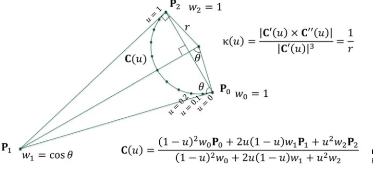
A circular arc (Fig. 3) is represented by a special case of rational quadratic Bézier curve with control vertices P0,P1,P2,

and parametric variable u∈[0, 1]. The weights of the vertices

are w0, w1, and w2, respectively, where w0=w2= 1 and

w1=cos(p/2−/P0P1P2/2). An exact representation of a

circu-lar arc is given by,

C(u) =(1−u) 2_P

0+2u(1−u)w1P1+u2P2

(1−u)2+2u(1−u)w1+u2 .

The convex hull property applies. Curvature κis defined by |C′×C′′|/|C′|3whereC′andC′′ are the first and second deriva-tives with respect tou. Radius is the reciprocal of curvature and both are constant for a circular arc. The central angle of an arc could be close to πradians in theory but for numerical stability in the computation, it is limited to about 2π/3. An arc with a wider central angle could be represented by a spline with two or three spans. Furthermore, a complete circle could be repre-sented by a rational quadratic periodic Bézier spline with three spans. Straight lines could also be represented as degenerate circu-lar arcs. Straight lines in either representation work equally well in this implementation.

Determination of curve–curve intersections

Point inversion and point projection (Piegl & Tiller, 1997, pp. 229–232) are used recursively on two curves to determine the minimum distance between them. If this distance is very small, it indicates an intersection has been found. Multiple seed values are used to ensure both intersections are found if there are two. Virtual intersections beyond the interval 0≤u≤1 are rejected. Given two curvesC(u)andD(t), and their seed values

P=D(t0) and Q=C(u0), the Newton–Raphson method is applied to a pair of parametric equations.

ui+1=ui−

C′(ui) · (C(ui) −P)

C′′(ui) · (C(ui) −P) + |C′(ui)|2

,

ti+1=ti−

D′(ti) · (D(ti) −Q)

D′′(ti) · (D(ti) −Q) + |D′(ti)|2.

Iteration continues until both point coincidence and zero cosine are satisfied, unless it is determined that there are no inter-sections. Two zero tolerances are used, a measure of Euclidean distance ε1= 10−8, and a zero cosine measureε2= 10−11. When the base unit of length is a meter,ε1denotes that any distance clo-ser than 0.01 µm is considered as coincident. Angle toleranceε2

implies that the modeling space is limited to a 1 km cube. No further tolerance analysis is performed. A pragmatic view was taken that there is sufficient precision to support processes like seeing and doing with paper and pencil, product design, and most architectural design purposes. These tolerances are taken from a popular solid modeling kernel, Parasolid. There is no need to differentiate curve–curve intersections from curve–line or line–line intersections.

Transformation matrices

This paper considers an initial shapeCand a shape ruleA→B. Automatic shape recognition relies on finding a complete list of transformations that satisfy t(A)≤C. Each transformation t is represented by a 4 × 4 homogeneous matrix which is defined by two sets of triple registration points (Fig. 4).

ShapeA (and shape B) is defined within a localuvw-frame. Three non-collinear points a1,a2,a3 from A are taken at each

time. The first point a1 is the local origin of shape A. Vector a1a2

_{denotes the u-direction. Vector a}

1a3

_{is on the uv-plane.} Their normalized cross-products are used to derive the orthogo-nal unit vectors uˆ,ˆv,wˆ of their uvw-frames. Each of them is denoted in terms of unit vectorsi,j,kfrom the globalxyz-frame.

ˆ u= a1a2

|a1|a2 ˆ

w= uˆ×a1a3

|uˆ×a1|a3 ˆ

v=wˆ ×uˆ

⎧ ⎪ ⎪ ⎪ ⎪ ⎪ ⎨ ⎪ ⎪ ⎪ ⎪ ⎪ ⎩

.

Likewise, shapeCis defined in a localabc-frame. Its origin and three orthogonal unit vectors,aˆ, bˆ, ˆc, are computed from three non-collinear registration points c4,c5,c6 from C. Translation

from the local origina1 of shapes Aand B to the global origin

is given by T−_A1. Rotation from the local uvw-frame to align with the global xyz-frame is given by T−_uvw1. If the mirror of a rule is used, matrix

M=

1 0

0 1

0 0

0 0

0 0

0 0

−1 0

0 1

⎡ ⎢ ⎢ ⎣

⎤ ⎥ ⎥ ⎦;

otherwise matrix M is an identity matrix. The proportional scaling factor s is used to define a scaling matrix S, where

s= |a1|a2/|c4|c5. Rotation from the global xyz-frame to align

with the local abc-frame is given byAabc. Translation from the

global origin to the local origin of shape C is given by TC.

Hence, a transformation,t, is represented by the following 4 × 4 homogeneous matrixT(Faux & Pratt,1979, pp. 70–78).

T=TCAabcSMA−uvw1T−A1.

Computational geometry in steps 1 and 4

Step 1 divides an initial shapeCinto atoms according to matching transformations that satisfy t(A)≤C. The input to this step is shape C, which is expected to be in maximal representation. If this condition cannot be ascertained, it is necessary to test and to combine elements if required to ensure all basic elements are maximal to one another (Krishnamurti,1980). By applying one valid transformation at a time, each basic element is divided into two or three relatively maximal parts or remains unchanged. Each part has the same original carrier curve. The original curve is defined with a parametric variable in the domain [0, 1]. Relatively maximal parts partition this into two or three non-overlapping domains joining end-to-end. Each atom consists of one or more Fig. 4.A transformationt represented by a 4 × 4

homogeneous matrixT.

relatively maximal parts. Output to this step is a list of symbolic references, each of which refers to an atom.

Step 4 applies a chosen shape rule under transformation t

(A)→t(B). The input to this step is a set grammar with the ruleA→Band a chosen transformationt. This results in an inter-mediate shapeC−t(A) in atoms andt(B) in one atom. The shape sum is computed from these two shapes. The resulting shape [C−t(A)] +t(B) is obtained after converting it into a maximal representation using computational geometry techniques such as joining multiple curve spans into a spline and knot insertion (Piegl & Tiller,1997, pp. 141–161). Hence, one shape rule appli-cation (Figs. 5b, 9b) of a shape grammar is accomplished. Both steps 1 and 4 are computational geometry operations.

Shape computation with set grammar in steps 2 and 3

Step 2 generates a lattice (Figs. 8,12). The input to this step is a set of atoms where each atom is referred to with a symbolic refer-ence and only this symbolic referrefer-ence is used in this step without any reference to its actual geometry. In this step, shape C is denoted by a set of all atoms, and is the supremum of the lattice. In step 3, a human user selects one from all valid transforma-tions. There are two possible ways to group and to present all possible transformation to a user. It could be either a list of all possible subshape matches (Figs. 6a,10a) or a list of visual equiva-lents of all possible resulting shapes (Figs. 6b,10b). The output of this step is a chosen transformation that applies to a shape rule. However, the presented shapes are in atomic form and are only visually equivalent to their maximally represented counterparts.

Two case studies

Two examples, the triangles grammar (Stiny,1994) and the trefoil grammar (Jowers & Earl,2010), are used to show how steps 2 and 3 are performed in practice.

The triangles grammar. One possible shape rule application (Fig. 5b) of a shape rule (Fig. 5a) is shown. ItsU13basic elements are straight lines. Five matches (Fig. 6a) produce five different

resulting shapes [C−t(A)] +t(B) (Fig. 6b). In fact, each match could be produced from 12 different transformations because of symmetry but, in this grammar, all 12 produce the same resulting shape. In step 2, shapeCis decomposed into six atoms (Fig. 7) and a complemented distributive lattice (Fig. 8) is generated that enumerates all possible matches of t(A) and their comple-ments, C−t(A). The triangles lattice (Fig. 8) has a height of 6 and 22 nodes in total.

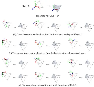
Because of the symmetries of the left- and right-hand shapes of rule 1, there are multiple transformations that produce the samet(B) but, in general, this is not the case. Here we consider all potential shape rule applications to the same equilateral triangle in the initial shape. Consider rule 2, which has the same left-hand shape as rule 1. Its right-hand shape does not have any symmetry and it is a solid inU33(Fig. 13a). The right-hand side of Rule 2 is an extrusion of the right-right-hand equilateral triangle of rule 1 plus an additional geometry to break the sym-metries. Rule 2 could be applied to the initial shape with three dif-ferent transformations from the front (Fig. 13b). Since the rule operates in a 3D space, three more shape rule applications could be made from the back (Fig. 13c). Since the mirror of a rule is also a valid rule, there are six more potential shape rule applications (Fig. 13d). There are altogether 12 valid transforma-tions since the left-hand shape of rule 2 is identical to that of rule 1. With rule 1, all 12 resulting shapest(B) are identical. However, with rule 2, all 12 t(B) are different. Hence, all the 12 resulting shapes [C−t(A)] +t(B) are different.

Decomposition of shapeC(Fig. 7) in connection with rule 1 is the basis for constructing the lattice (Fig. 8). The way in which this decomposition is made is the same as for the trefoil grammar and described in the next section. In the current implementation, step 3 is carried out by a user who manually selects from the pos-sible rule applications identified in step 2.

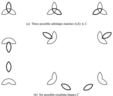
Trefoil grammar. A similar sequence is shown for the trefoil grammar (Fig. 9). ItsU13 basic elements are circular arcs. Three matches (Fig. 10a) produce six different resulting shapes [C− t(A)] +t(B) (Fig. 10b). In fact, each match could be produced from eight different transformations. The shapeChas six atoms (Fig. 11). The complemented distributive lattice generated in step 2 (Fig. 12) enumerates all possible matches of t(A) and their complements C−t(A). The trefoil lattice (Fig. 12) has a height of 4 and 20 nodes.

The lattice for this grammar differs from the previous one, even though both have six atoms. This is because the left-hand Fig. 7.Decomposition of the initial shapeCof the shape grammar of triangles into six

atoms.

side shapesA of the triangles grammar consist of two atoms in some cases or three atoms in others, whereas, the left-hand side shapeA of the trefoil grammar consists of three atoms for each matchingt(A). This shows how the generated lattice structure var-ies according to the initial shape, and the left-hand side of a shape rule.

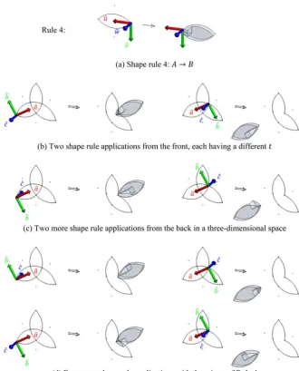
Similar to rules 1 and 2, the relationship between rules 3 and 4 are used demonstrate the effect of symmetries of the left- and right-hand shapes, or the lack of them. Here we consider all potential shape rule applications to the same leaf in the initial shape. Rule 4 (Fig. 14a) could be applied twice from the front (Fig. 14b) and twice from the back (Fig. 14c). With the mirrored rule, there are four further valid transformations (Fig. 14d). With rule 3, there are eight valid transformations for one leaf of the initial shape and there are two different t(B). However, with rule 4, there are eight differentt(B) and, therefore, eight different resulting shapes.

As with the triangles grammar, in the current implementation, step 3 is carried out by a user who manually selects from the pos-sible rule applications identified in step 2.

A note on 2D versus 3D shape rules

Both the triangles grammar and the trefoil grammar were origi-nally defined inU12algebra. By translating them intoU13algebra, we are able to show the effect of symmetries of the left-hand shape

A and right-hand shape B. There are more matches in three dimensions that do not exist in two dimensions.Figures 13,14

show the effect of lack of symmetry of the right-hand shape B. With Rule 1 (Fig. 5a), for every one of the five matched triangles, there is one distinct right-hand shape (Fig. 6b) whereas with rule 2, there are 12 (Fig. 13b–d). With rule 3 (Fig. 9a), for each one of the three matched leaves, there are two distinct right-hand shapes (Fig. 10b) whereas with rule 4, there are eight (Fig. 14b–d). Fig. 8.Lattice of the initial shapeCof the triangles grammar decomposed by Rule 1.

From basic elements to relatively maximal parts to atoms The process of set grammar computation with the triangles grammar and that of the trefoil grammar are similar, but the basic elements used in trefoil grammar are more complex. Details of the trefoil grammar computation are described here as an example. The same general principle of decomposition applies to both grammars.

The initial shape (Fig. 2a) of the trefoil grammar in maximal representation has three basic elements C= {U, T, V} (Fig. 2b). Superimposing each of the three matches of t(A) onto C in turn, each basic element is divided into three relatively maximal parts. Hence,C= {{u1,u2,u3}, {t4,t5,t6}, {v7,v8,v9}} has nine rel-atively maximal parts (Fig. 2c). The parts ofCare relatively max-imal to one another but C is not in maximal representation anymore. Each of the three subshape matches can be produced from eight different transformations. Each set of eight transfor-mations produces the samet(A). Some combinations of these rel-atively maximal parts form partitions. All parts of a partition are either all subshapes oft(A) orC−t(A), but not both and not par-tially in or out. Each partition of relatively maximal parts is called an atom. The analog of an atom is useful here. An atom could consist of more than one relatively maximal part, but it is the smallest indivisible unit in the context of a set grammar derived from a shape grammar under all possible t(A) matches in an initial shape C. Shape C of this set grammar has six atoms (Fig. 2d), which constitute shape C= {u2,v8, t5, {t6,v9}, {u3,t4}, {u1, v7}}. We can rename these atoms as C= {a, b, c, d, e, f} (Fig. 2d) which correspond to the previous partitions. There are 24 transformations,t1,t2,…,t24, that satisfyt(A)≤C. We select three (Fig. 2e–g) transformations that have three differentt(A). They aret3(A) = {b,c,d},t7(A) = {a,b,f},t11(A) = {a,c,e}.

Among the eight transformations that would produce at(A) that is the same as t3(A), four of them would have the same

t(B), and the other four have a differentt(B). There are altogether six possible t(B) as shown inFigure 10b, which aret3(B),t7(B),

t11(B),t15(B),t19(B),t23(B). Among all 24 valid transformations, there are six distinct set grammar computations using symbolic references to relatively maximal parts (Table 2). Three matches of t(A)≤C are shown in Figure 10a. The six resulting shapes [C−t(A)] +t(B) are shown inFigure 10b.

Relatively maximal parts ofCare recombined to form atoms using all matching transformations. These are computed from the algorithm shown below.

Fig. 10.Different shape computations of the trefoil grammar.

Fig. 11.Decomposition of the initial shapeCof the trefoil grammar into six atoms.

ONEpartition_of_C←relatively_maximal_parts_of_C

FOR EACHtransformation

basic_elements_of_t(A)←transformationOFbasic_elements_of_A

FOR EACHpartition_of_C

set_intersect←partition_of_C∩basic_elements_of_t(A)

set_difference←partition_of_C\basic_elements_of_t(A)

THISpartition_of_C ←set_intersect

NEWpartition_of_C←set_differenceUNLESS EMPTY SET

END FOR EACH END FOR EACH

EACHatom_of_C←EACHpartition_of_C

Then, eacht(A) is rerepresented using the symbolic references of the atoms of C.

FOR EACHtransformation

basic_elements_of_t(A)←transformationOFbasic_elements_of_A

FOR EACHatom_of_C

basic_elements_of_an_atom←ELEMENTS OFatom_of_C

atoms_of_t(A)←EMPTY SET

FOREACHbasic_elements_of_atom

IF ALLbasic_elements_of_an_atomIS INbasic_elements_of_t(A)

atoms_of_t(A)←atoms_of_t(A) +atom_of_C

Discussion

Implementation details related to the representation of basic ele-ments, their division into relatively maximal parts, and the use of control vertices to describe circular arcs are considered in the first three parts of this section. The final two sections compare this implementation with that of the quad interpreter (QI) and con-sider the benefits of using a generalized description ofU13basic elements.

Representation of basic elements

Two different types of basic element (parametric curve) were used in this implementation: straight line, and circular arc up to a sub-tending angle of 2π/3. Both are represented by a parametric equa-tion which is defined with its parametric variable for the interval [0,1]. A straight line is a constant speed curve with respect to its parametric variable. A circular arc type basic element is repre-sented by a quadratic rational Bézier curve. If the maximum sub-tending angle is limited to 2π/3, its speed deviates by 19% at the most. A circular arc type basic element could be degenerated into

a straight line type if the middle control vertex is coincident with the line adjoining the first and third vertices, and/or the weight of the second vertex is set to zero. A circular arc with a wider subtending angle is represented by a Bézier spline with two or three spans. In terms of finding intersection(s) of any two basic elements, the type of U13 basic element is immaterial. Exactly the same routine is used since all of them are in maximal repre-sentation and defined when their parametric value is within the interval [0, 1].

Dividing a basic element into its relatively maximal parts

with a parametric variable in the interval [0, 1] whereas, the two relatively maximal parts are defined in the intervals of [0, 0.5] and [0.5, 1] using the same carrier curve/line. It is advantageous not to change the carrier curve but simply specifying different ranges of a parametric variable. This is significantly different from previous implementations. It is similar to the use of collinear maximal lines as a descriptor or a carrier line used by Krishnamurti and Earl (1992). But instead of spelling out the coordinates of the end-points of lines/curves, a single value of a parametric variable used. In turn, by applying a parametric value onto curves, the 3D coordinates of the required point can be determined.

Figures 11,2cshows each of the three circular arcs divided into three relatively maximal parts. The use of parametric curves in this work is essentially the same as that of Jowers and Earl (2010). The main difference is that we do not require new control polygons for any new relatively maximal parts; instead, we vary the ranges of the parametric variable on the same carrier line, curve or spline.

Figure 2cshows each of the three circular arc type basic elements divided into three relatively maximal parts. The ranges of their parametric variables are [0, 0.41], [0.41, 0.59], and [0.59, 1].

Control vertices of a rational quadratic Bézier curve

A quadratic Bézier curve (Fig. 3) in general has three control ver-tices,P0,P1,P2. In this paper, circular arcs are represented by a

special case of a rational quadratic Bézier curve. The middle con-trol vertex lies on the perpendicular divider of the line P0P2

adjoining the first and last control vertices, where their weights are set to unity,w0=w2= 1. The weight of the middle vertex is set to a value such that this rational curve is an exact representa-tion of a circular arc, that is, w1=cos(p/2−/P0P1P2/2).

Degeneration of a circular arc to form a straight line is allowed by positioning the middle vertex to lie on the midpoint ofP0P2

and/or setting the weight of the middle vertex to zero, that is,

w1= 0. This is effectively degree elevation (Piegl & Tiller,1997, pp. 188–212) that allows algorithms designed for rational quad-ratic curves to operate correctly on non-rational linear curves.

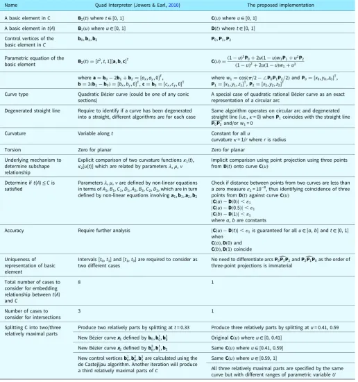
Comparison between QI and the proposed approach

it is divided into two or three relatively maximal parts depending exactly how the two basic elements are embedded.

When QI divides a basic element into two or three relatively maximal parts, each part is defined by a new control polygon. De Castejljau’s algorithm is used to compute the new control ver-tices. Each relatively maximal part is defined when the para-metric variable is within the interval [0, 1]. In this paper, when a basic element is divided into its relatively maximal parts, all parts are represented by the same parametric curve

of the original basic element, but they are defined by discrete and complementary intervals, for example, [0, a], [a, b], and [b, 1], wherea,bare the parametric values where the basic ele-ment splits. There are several implications of these two approaches.

Firstly, in QI a quadratic Bézier curve is represented by a para-metric equation,B2(t) =t2a+tb+c, wherea,b,care defined in

terms of the control verticesb0,b1,b2, to represent a curve of a

conic section. In this paper, we used the rational form of another Fig. 14.Eight matching transformationstand eight

corre-sponding resulting shapest(B) for shape rule 4:A→B.

Table 2.Shape computation in a set grammar using symbolic references

C t(A) C−t(A) [C−t(A)] +t(B)

C= {a,b,c,d,e,f} t3(A) =t15(A) ={b,c,d} {a,e,f} {a,e,f} +t3(B)

{a,e,f} +t15(B)

C= {a,b,c,d,e,f} t7(A) =t19(A) = {a,b,f} {c,d,e} {c,d,e} +t7(B)

{c,d,e} +t19(B)

C= {a,b,c,d,e,f} t11(A) =t23(A) = {a,c,e} {b,d,f} {b,d,f} +t11(B)

parametric equation C(u) = (1−u)2_P

0+2u(1−u)P1+u2P2,

whereP0,P1,P2are the control vertices, as an exact representation

of a circular arc.

Secondly, in QI, the embedding relation of two basic ele-ments, one fromt(A) and the other from C, is determined by intrinsic comparison of curvatures. The curvature of each basic element is represented by an explicit function with four coeffi-cientsA, B, C, Dfor each curve. In turn, these coefficients are defined by non-linear equations in terms of a,band ultimately

b₀,b₁,b₂. Two curvature functions are related by parametersλ,

μ, ν which are defined in terms of coefficients A1, B1, C1, D1,

A2,B2,C2,D2. In contrast to the proposed approach, the embed-ding relation is determined by projecting three points from the element oft(A) onto the element ofC. If the minimum distances between all three point projections are less than a zero measure

ε1= 10−8, the embedding relation is deemed to be satisfied With one or both ends of the element fromt(A) acting as the splitting points for the element from C. This could result in one, two, or Table 3.Comparison between QI and the proposed approach

Name Quad Interpreter (Jowers & Earl,2010) The proposed implementation

A basic element in C B2(t)wheret∈[0, 1] C(u)whereu∈[0, 1]

A basic element int(A) B1(u)whereu∈[0, 1] D(t)wheret∈[0, 1]

Control vertices of the basic element inC

b0,b1,b2 P0,P1,P2

Parametric equation of the

basic element B2(t) =[t

2_{,t, 1][a,b,c]}T _{C(u) =}(1−u) 2

P0+2u(1−u)w1P1+u2P2

(1−u)2_+2u(1−u)w

1+u2

wherea=b0−2b1+b2=[ax,ay, 0]T, b₌2(b1−b0) =[bx,by, 0]T,c=b0=[cx,cy, 0]T

wherew1=cos(p/2−/P0P1P2/2)andP0=[x0,y0,z0]T,

P1=[x1,y1,z1]T,P2=[x2,y2,z2]T

Curve type Quadratic Bézier curve (could be one of any conic sections)

A special case of quadratic rational Bézier curve as an exact representation of a circular arc

Degenerated straight line Require to identify if a curve has been degenerated into a straight, different algorithms are for each case

Same algorithm operates on circular arc and degenerated straight line (i.e.,κ= 0) whenP1coincides with the straight line

P0P2and/orw1= 0

Curvature Variable alongt Constant for allu

curvatureκ= 1/rwhereris radius

Torsion Zero for planar Zero for planar

Underlying mechanism to determine subshape relationship

Explicit comparison of two curvature functionsκ1(t),

κ2[u(t)] which are related by parametersλ,μ,ν Implicit comparison using point projection using three pointsfromD₍t)onto curveC₍u)

Determine ift(A)≤Cis satisfied

Parametersλ,μ,νare defined by non-linear equations in terms ofA1,B1,C1,D1,A2,B2,C2,D2, which are in turn defined by non-linear equations involvinga1,b1,a2,b2

Check if distance between points from two curves are less than a zero measureε1= 10−8, thus identifying coincidence of three points fromD(t)against curveC(u)

|C(a) −D(0)|,11

|C(u) −D(0.5)|,11

|C(b) −D(1)|,11

wherea,bare constants

Accuracy Require further analysis |C(u) −D(t)|,11is guaranteed for allu∈[a,b] andt∈[0, 1] when

C(a),D(0)and

C(b),D(1)coincide

Uniqueness of representation of basic element

Intervals [t0,t1] and [t1,t0] are required to consider as two different cases

No need to differentiate arcsP0P1P2andP2P1P0as the order of three-point projections is immaterial

Total number of cases to consider for embedding relationship betweent(A) andC

8 1

Number of cases to consider for intersections

3 1

Splitting C into two/three relatively maximal parts

Produce two relatively parts by splitting att= 0.33 Produce three relatively parts by splitting atu= 0.41, 0.59

New Bézier curvex1defined byb0,b10,b 2

0 OriginalC(u)whereu∈[0, 0.41] New Bézier curvex2defined byb20,b

1

1,b2 SameC(u)whereu∈[0.41, 0.59] New control verticesb10,b20,b11are calculated using the

de Castejljau algorithm. Another iteration will produce a third relatively maximal parts ofC

SameC(u)whereu∈[0.59, 1]

three relatively maximal parts of C. The proposed approach is simpler in terms of dividing a basic element into its part for later use. The original basic elements and its relatively maximal parts share the same carrier curves but with different parameter ranges.

Thirdly, QI considers Bézier curves as distinct from straight lines, so degeneration of a Bézier curve into a straight is not per-mitted. For this reason, curve–curve, curve–line, and line–line intersections are considered as three different cases. Numerical stability when a curvature is close to zero was not investigated but it is likely to be necessary to impose a minimum curvature limit to avoid division by numbers close to zero. As a result, two different algorithms are required: one for Bézier curves and the other one for straight lines. In this paper, a degenerate straight line can be represented as a Bézier curve (as outlined in the sub-section “Control vertices of a rational quadratic Bézier curve”). With the proposed approach, whether a basic element is a true curve or a straight line is immaterial. They can be dealt with by the same algorithm equally well and, whatever the actual geome-try, only one algorithm is necessary for intersections between any two basic elements of any type. Fourthly, for a particular embed-ding relation, QI is required to determine, which one among all eight possible ways, one basic element is embedded within another one. The ordering of the parametric variables of each curve is important. In this paper, a coincidence test of three points on a curve is needed for testing the embedding relation. The order of testing each of the three points is immaterial. The direction of the parametric variable is immaterial too.

Finally, the most important aspect of the proposed imple-mentation is the use of atoms. QI repeats the above operation for each matching transformation while in this work, a set of atoms and shapes derived from them form a lattice. Each match-ingt(A), among other shapes, is already a node in this lattice.

Benefits of a generalized description ofU13basic elements

In concluding the discussion of implementations for general (Bézier) curves and circular arcs, we note that the example of the trefoil grammar is a special case for the application of the general curve grammar. However, the circular arc implementation concen-trates on addressing the specific geometrical elements arising in the trefoil configurations. In design applications of shape grammars, there is a tension between creating tools specific to geometrical ele-ments of interest and more general tools applicable across a wider range of geometric elements. This paper has demonstrated that limiting geometrical elements can focus attention on the details of where and how emergence occurs as well as the necessary shape computations to implement it in a design context. In par-ticular, the paper indicates that a separation between geometric cal-culation and shape computation assists the development of usable and extensible tools for shape grammar implementation.

Conclusions and future work

The ideas presented in this paper came from research on the use of hypercube lattices to support the configuration of bills of materials (BOMs) in engineering product development processes (Kodama et al.,2016). Important benefits of using lattices for the configura-tion of BOMs are that they provide: (i) a self-consistent computa-tional space within which BoMs can be manipulated and (ii) connectivity to the source design description that allows users to move back and forth between BOMs and other forms of design

description. The type of relationship between parts in a BOM (part–whole relationships) is the same as that between shapes and sub-shapes in shape grammars. This led to us exploring a potential application to shape grammar implementation.

The significance of the proposed approach for software imple-mentation of shape grammars is that computational geometry and shape computation are decoupled. A temporary set grammar is gen-erated using an initial shape and a shape rule and represented as a complemented distributive lattice. All occurrences of the left-hand side of the rule in the initial shape are nodes in the lattice. For this rea-son, shape computation can be performed without considering the actual geometries of the shapes involved. Decoupling the geometry and grammar has resulted in two desirable outcomes. Firstly, shape algebra operations–shape difference and shape sum–are equivalent to complements and joins of nodes in the lattice. This allows the results of shape algebra operations to be derived from the lattice rather than calculated. Secondly, an extension to include more types of shape element will not change the shape computational aspect of a shape grammar implementation. A new set grammar is generated for each rule application in a given shape computation process.

A medium-term objective of the presented approach is to allow shape grammar to be used in domains that require freeform geo-metries, for example, consumer products. In a wider context, shape emergence and calculation with shapes have been studied by scholars from different disciplines (Wittgenstein, 1956; Stiny,

1982; Tversky,2013). Minsky’s (1986, p. 209) enquiry on visual ambiguity and Stiny’s (2006; p. 136) different views on the Apple Macintosh logo examples are examples of multiple interpretations. This research brings closer software tools that realize the potential of calculation with shapes for theoretical studies as well as laying a foundation for practical tools in various spatial design contexts.

Acknowledgments. This research is supported by the UK Engineering and Physical Sciences Research Council (EPSRC), under grant number EP/ N005694/1,“Embedding design structures in engineering information”. We are also grateful to the anonymous reviewers for their constructive comments.

References

Ben Yahia S and Konecny J (eds) (2015) The Twelfth International Conference on Concept Lattices and Their Applications (CLA 2015), Clermont-Ferrand, France, 13–16 October 2015.

Berge C(1973)Graphs and Hypergraphs. Amsterdam: North-Holland.

Chase SC(1989) Shape and shape grammars: from mathematical model to computer implementation. Environment and Planning B: Planning and Design16(2), 215–242.

Chase SC(2010) Shape grammar implementations: the last 36 years. Shape grammar implementation: from theory to useable software. In Design Computing and Cognition (DCC’10) Workshop, Stuttgart, 11 July 2010.

Chau HH, Chen X, McKay A and de Pennington A(2004) Evaluation of a 3D shape grammar implementation. In Gero JS (ed.).Design Computing and Cognition’04. Dordrecht, The Netherlands: Kluwer, pp. 357–376.

Faux ID and Pratt MJ (1979) Computational Geometry for Design and Manufacture. Chichester, UK: Ellis Horwood.

Ganter B and Wille R (1999) Formal Concept Analysis: Mathematical Foundations. Berlin: Springer.

Gips J(1999) Computer implementations of shape grammars. InNSF/MIT Workshop on Shape Computation, Cambridge, MA, April 1999.

Grasl T (2012) Transformational palladians.Environment and Planning B: Planning and Design39(1), 83–95.

Grasl T and Economou A(2013) From topologies to shapes: parametric shape grammars implemented by graphs.Environment and Planning B: Planning and Design40(5), 905–922.

Huchard M and Kuznetsov SO (eds) (2016) The Thirteen International Conference on Concept Lattices and Their Applications (CLA 2016), Moscow, Russia, 18–22 July 2016.

Jowers I and Earl CF(2010) The construction of curved shapes.Environment and Planning B: Planning and Design37(1), 42–58.

Jowers I and Earl CF(2011) Implementation of curved shape grammars.

Environment and Planning B: Planning and Design38(4), 616–635.

Jowers I, Hogg DC, McKay A, Chau HH and de Pennington A(2010) Shape detection with vision: implementing shape grammars in conceptual design.

Research in Engineering Design21(4), 235–247.

Kodama T, Kunii TL and Seki Y(2016) A case study of homotopic BOM information management using the cellular data system. In IEEE Congress on Evolutionary Computation (CEC), 24–29 July 2016. pp. 4501–4507.

Krishnamurti R(1980) The arithmetic of shapes.Environment and Planning B: Planning and Design7(4), 463–484.

Krishnamurti R (1981) The construction of shapes. Environment and Planning B: Planning and Design8(1), 5–40.

Krishnamurti R(1992) The maximal representation of shapes.Environment and Planning B: Planning and Design19(3), 267–288.

Krishnamurti R and Earl CF(1992) Shape recognition in three dimensions.

Environment and Planning B: Planning and Design19(5), 585–603.

Krstic D (2010) Approximating shapes with hierarchies and topologies.

Artificial Intelligence for Engineering Design, Analysis & Manufacturing,

24(2), 259–276.

Krstic D (2016). From shape computations to shape decompositions. In Gero JS (ed.).Design Computing and Cognition‘16. Switzerland: Springer, pp. 263–281.

Li AI-K, Chau HH, Chen L and Wang Y(2009) A prototype system for devel-oping two- and three-dimensional shape grammars. In Chang T-W, Champion E, Chien S-F and Chiou S-C (eds).CAADRIA 2009: Proceedings of the 14th International Conference on Computer-Aided Architecture Design Research in Asia, Touliu, Taiwan. Taiwan: Department of Digital Media Design, National Yunlin University of Science & Technology, pp. 717–726.

March L(1983) Design in a universe of chance.Environment and Planning B: Planning and Design10(4), 471–484.

March L(1996) The smallest interesting world?Environment and Planning B: Planning and Design23(2), 133–142.

McKay A, Chase S, Shea K and Chau HH(2012) Spatial grammar implemen-tation: from theory to useable software.Artificial Intelligence for Engineering Design, Analysis & Manufacturing26(2), 143–159.

Minsky M(1986)The Society of Mind. New York: Simon & Schuster.

Piegl L and Tiller W(1997)The NURBS Book, 2nd edn, Berlin: Springer.

Rovetto RJ(2011) The shape of shapes: an ontological exploration. In Kutz O, Hastings J, Bhatt M and Borgo S (eds).SHAPE 1.0: The Shape of Things, Paper 9, Karlsruhe, Germany, 27 September 2011. CEUR-WS Volume 812.

Rudolph S(2006) A semantic validation scheme for graph-based engineering design grammars. In Gero JS (ed.). Design Computing and Cogntion’06. Dordrecht, The Netherlands: Springer, pp. 541–560.

Ruiz-Montiel M, Mandow L, Pérez-de-la-Cruz J-P and Gavilanes J(2011). Shapes, grammars, constraints and policies. In Kutz O, Hastings J, Bhatt M and Borgo S (eds).SHAPE 1.0: The Shape of Things, Paper 4, Karlsruhe, Germany, 27 September 2011. CEUR-WS Volume 812.

Simons P(1987)Part: A Study in Ontology. Oxford, UK: Oxford University Press.

Stiny G(1982) Spatial relations and grammars.Environment and Planning B: Planning and Design9(1), 113–114.

Stiny G(1991) The algebras of design.Research in Engineering Design2(3), 171–181.

Stiny G(1994) Shape rules: closure, continuity, and emergence.Environment and Planning B: Planning and Design21, s49–s78.

Stiny G(2006)Shape: Talking about Seeing and Doing. Cambridge, MA: MIT Press.

Strobbe T, Pauwels P, Verstraeten R, De Meyer R and Van Campenhout J

(2015) Toward a visual approach in the exploration of shape grammars.

Artificial Intelligence for Engineering Design, Analysis & Manufacturing,

29(4), 503–512.

Szász G (1963) Introduction to Lattice Theory. Budapest: The Publishing House of the Hungarian Academy of Sciences.

Tapia MA (1999) A visual implementation of a shape grammar system.

Environment and Planning B: Planning and Design26(1), 59–73.

Tversky B(2013) Lines, shapes, and meaning. In Kutz O, Bhatt M, Borgo S and Santos P (eds). SHAPE 2.0: The Shape of Things. pp. 41–45. Workshop held at the World Congress and School on Universal Logic, Rio de Janerio, Brazil, April 3–4, 2013. CEUR-WS Volume 1007.

Wittgenstein L(1956)Remarks on the Foundations of Mathematics. Oxford, UK: Basil Blackwell.

Yue K and Krishnamurti R(2013) Tractable shape grammars.Environment and Planning B: Planning and Design40(4), 576–594.

Hau Hing Chauis a teaching fellow in the School of Mechanical Engineering at the University of Leeds. He obtained his PhD in 2002 from the University of Leeds on the preservation of brand identity in engineering design using a grammatical approach. Since then, his research has focused on shape com-putation and the implementation of 3D shape grammar-based design sys-tems for use in the consumer product development processes.

Alison McKayis a Professor of Design Systems in the School of Mechanical Engineering at the University of Leeds. Her research focus on three kinds of design system: shape computation and information systems used to create designs and develop products, and the socio-technical systems within which designers work and in which their designs are used. Her research is posi-tioned within the context of stage-gate processes that typify current industry practice and aims to facilitate improved modes of working through the exploitation of digital technology and to establish design methods, and tools to support systematic evaluation of design alternatives at decision gates.

Christopher Earlhas been a Professor of Engineering Design at the Open University since 2000. He obtained his PhD in design from the Open University and works closely with a wide range of research groups in design and shape computation worldwide. Prior to 2000, he held positions at Newcastle University, affiliated with the Engineering Design Centre in the Faculty of Engineering, where his research concentrated on the design and man-ufacture processes for large, complex, engineering to order products, particu-larly their planning and scheduling under uncertainty. Dr Earl’s main research interests are in generative design, models of design processes, and com-parisons across design domains.

Amar Kumar Beheraholds BTech, MTech, and minor degrees from Indian Institute of Technology, Kharagpur; MS from the University of Illinois, Urbana-Champaign; and PhD from the Katholieke Universiteit Leuven. He joined Mphasis an HP company in 2008 and later worked as an Assistant Professor at Birla Institute of Technology and Science, Pilani, and a research fellow at the University of Nottingham. Since 2015, he has been with the University of Leeds, where he is a research fellow. His main areas of research interest are digital manufacturing and design informatics. Dr Behera is an associate fellow of the UK Higher Education Academy and has published 35 peer-reviewed articles.