This is a repository copy of A simple account of the complex may take a while : Review of: Stump, Gregory T. & Raphael A. Finkel, Morphological typology: from word to paradigm (= Cambridge Studies in Linguistics 138). Cambridge: Cambridge University Press, 2013. xxiv + 402pp. ISBN: 978-1-107-02924-8 (hardback)..
White Rose Research Online URL for this paper: http://eprints.whiterose.ac.uk/122965/
Version: Accepted Version
Article:
Brown, Dunstan Patrick orcid.org/0000-0002-8428-7592 (2018) A simple account of the complex may take a while : Review of: Stump, Gregory T. & Raphael A. Finkel,
Morphological typology: from word to paradigm (= Cambridge Studies in Linguistics 138). Cambridge: Cambridge University Press, 2013. xxiv + 402pp. ISBN: 978-1-107-02924-8 (hardback). Word Structure. pp. 238-53. ISSN 1750-1245
eprints@whiterose.ac.uk https://eprints.whiterose.ac.uk/ Reuse
Items deposited in White Rose Research Online are protected by copyright, with all rights reserved unless indicated otherwise. They may be downloaded and/or printed for private study, or other acts as permitted by national copyright laws. The publisher or other rights holders may allow further reproduction and re-use of the full text version. This is indicated by the licence information on the White Rose Research Online record for the item.
Takedown
If you consider content in White Rose Research Online to be in breach of UK law, please notify us by
A simple account of the complex may take a while
Stump, Gregory T. & Raphael A. Finkel, Morphological typology: From word to paradigm
(= Cambridge Studies in Linguistics 138). Cambridge: Cambridge University Press, 2013.
xxiv + 402pp. ISBN: 978-1-107-02924-8 (hardback).
Reviewed by DUNSTAN BROWN
Keywords: default, entropy, inflectional class, morphological complexity
1. Overview
Morphological typology: From word to paradigm (MT) was published five years ago. Since
then it has already been widely accessed within the community of scholars working on
morphological theory. Software on the site associated with the book is a useful source for
assessing and evaluating inflectional class systems. Given the time since publication it is also
to be expected that MT has been reviewed, for instance by Dahl (2014). Dahl indicates that
he did not find the book easy reading. There may be some justification to this view, but I
would like to suggest that MT provides us with the means to understand paradigms and their
organisation in ways that have never before been available, and that it is worth the effort of
the community of scholars researching morphology to build on the highly innovative work in
MT and examine further what the different complexity measures mean, and how they can be
used to formulate typologies. It is hardly surprising that morphological complexity is a
challenge to understand, and a complete and overarching account of the topic is probably still
a long way off. But anyone who wishes to develop such an account needs to engage with the
fundamental ideas and methods that are made available in MT.
Before progressing to our discussion of MT we need first to be clear about the
questions that the book addresses. As its title suggests, MT provides a typology of
The structures in question, as the subtitle makes clear, involve the relationship between words
and paradigms. Above all, the book is about the typological classification of paradigms and
the implicative relations that they involve. It provides several different ways of measuring the
variation exhibited in inflectional class systems, and morphological complexity is a key
concept that lies at the heart of this.
There are a myriad different ways in which the term COMPLEXITY can be used, both in
linguistics and beyond. So it is important to understand the domain covered by the term in
MT. In MT complexity is associated with inflection classes. Languages with inflectional
morphology but no inflectional classes, such as Turkish, are excluded from this notion of
complexity, just as much as languages without any inflectional morphology (p. 11). Stump &
Finkel aim to characterise the complexity of inflectional class systems according to how
straightforwardly the different forms of a lexemes can be inferred:
Our objective in this monograph is to propose a clear conception of an IC [inflection
class] system’s complexity, as the extent to which it inhibits motivated inferences about
a lexeme’s full realized paradigm from subsets of its cells. (p. 21)
Under such a construal of complexity a highly complex inflectional class system is one where
the Paradigm Cell Filling Problem (Ackerman, Blevins & Malouf 2009, Ackerman & Malouf
2013) is a big problem. A major contribution of MT to this matter is the development of a
number of measures of IC system complexity. Stump & Finkel emphasize that their
approach, because it is based on principal parts, is about certainty, rather than probability.
The emphasis on inference could bring with it assumptions about what is easy or hard for
speakers, but the measures are really about structural properties of languages, specifically
paradigms. In fact, the investigation of how the measures relate to the processing and
learning of languages would present a very rich seam for investigation. The individual
the full set of forms of lexemes in different ways. In my view, making available measures
that highlight different aspects of morphological complexity is a key part of MT’s value. The
ongoing task is to understand these measures better, determining how they pick out different
sub-types of complexity and assessing their value for morphological typology. As Bane
(2008: 75) has noted, ‘in a sense, it doesn’t really matter whether a metric truly corresponds
to whatever we mean by “complexity,” as long as it is useful.’ Bearing this point in mind, we
need to be clear that the reason why IC system complexity, as discussed in MT, is interesting
is because it represents an additional layer of structure that appears to be unnecessary.
Indeed, it inhibits reliable inferences about inflectional forms. Our purpose should therefore
be to see where the variation lies in languages with IC systems and which of the measures in
MT can be used to describe that typological space. We first consider the different measures in
section 2, then focus in section 3 on some of the predictions in MT. Representational issues
are a major challenge in the area of morphological complexity, and MT has much of value to
say on this, something we discuss in section 4. In section 5 we give an indication of key ideas
arising from MT that should influence future direction in the field, in particular the hybrid
model developed, and the subtly different notions of complexity that the measures pick out.
Stump & Finkel (p. 314) argue that the measures that they develop are not reducible
into each other. In Chapter Eleven they apply ten measures to twelve different inflectional
class systems. As it is important to understand how much of the space of morphological
complexity that MT allows us to account for, we look at these measures and discuss them in
turn.
2. The ten correlates of inflectional class systems’ complexity
As we progress through the correlates and associated measures, I give an indication of how
they can be seen in terms of a simple dichotomy between rules and listing. This is not how
relation to these ideas, given that morphology in a certain sense represents a compromise
between lexical specification (or listing) on the one hand, and rules (or implicative relations)
on the other.
The first of the ten measures presented in their outline of typological variation in
morphological complexity is the number of distillations:
(1) ‘The more distillations an IC system has, the more complex it is.’ (p. 327)
Distillation is a key concept in MT, first introduced in Chapter Two (p. 42). The set of feature
values that define a paradigm cell, morphosyntactic property sets (MPS) in Stump & Finkel’s
terms, give us information about inflectional class distinctions. Where one MPS distinguishes
the classes in the same way as another MPS, these are isomorphic and can be reduced to one
distillation. As a real-life example of this, consider the prefixal marking of gender and
number in Burmeso in Table 1 (based on Donohue 2001: 100, 102).
INSERT TABLE 1 ABOUT HERE
There are two inflectional classes in Table 1 (represented in the rows by the example lexemes
‘see’ and ‘bite’). Each MPS, corresponding to a column, makes the same number of
inflectional class distinctions (here two). This means that the twelve MPS in Table 1 can be
reduced to one distillation. The Burmeso example in Table 1 is therefore not complex when
evaluated from the perspective of (1).1 More distillations indicate that inflectional classes are
not isomorphic, and therefore that the structure of the IC system is complex. In MT (p. 41)
distillations are presented in terms of redundancy within MPSs: The MPSs in a distillation
share the same class structure and are therefore redundant. Another way of looking at it is to
consider the number of MPS and distillations in relation to each other, something that can
indicates to us how many MPSs contribute to the inflectional system actually being an IC
system. We might interpret this as telling us something about how much of the rule system
requires purely morphological information.
The next measure of morphological complexity, as noted by Stump & Finkel, correlates
loosely, but imperfectly, with the number of distillations:
(2) ‘The larger the size of an IC system’s optimal static principal-part sets, the more
complex it is.’ (p. 327)
Static principal parts correspond to the traditional notion of principal part that we are familiar
with from pedagogical grammars: The learner needs to know a specified number of forms in
order to work out the rest of the paradigm. Of course, this fails to take into account the fact
that for some lexemes we can get away with knowing less than for others (something dealt
with by the dynamic principal parts system introduced elsewhere in MT, and discussed later
in this section). Stump & Finkel note that the Icelandic conjugational system requires eight
static principal parts. We could construe this type of measure as telling us something about
the lexical listing that is required in order to facilitate the rule system. One of the reasons why
it is important to interpret the size of the static principal parts set in relation to the number of
distillations is that the latter gives us an indication of how much work the principal parts have
to do, again indicating how the rule system and the listed parts need to interact.
One of the most interesting aspects of IC systems is the implicational overlap of cells in
predicting each other. In a simplistic model of morphology one set of forms are listed and are
used to predict another, disjoint, set of forms. However, in the real morphological world
things are not that simple. There may be alternative static principal parts analyses, and MT
provides a density measure for this:
(3) ‘The lower the density of an IC system’s optimal static principal-part sets, the more
Returning to the Icelandic example, the size of the static principal parts set is 8. The number
of distillations for Icelandic is 21. (In contrast, there are 30 MPSs in the dataset for
Icelandic.) There are 60 alternative combinations of 8 principal parts that work for Icelandic.
The number of possible combinations of 8 principal parts that could be chosen from the 21
distillations is 203,490.2 The density is the ratio of actual to possible static principal parts sets
(60/203,490), which is less than 0.001, the lowest of all the twelve case-study languages in
MT. As Stump & Finkel note, measures based on static principal parts, such as the density
measure in (3), are not entirely satisfactory, because the requirement that the number of
principal parts always be the same inflates the size of the principal parts set. This also means
that for some lexemes the cells included in the principal parts set are not doing that much
work, because of the implicational overlap. The reason why lower density static principal
parts sets are considered more complex is because this indicates that the choice of viable
combinations of cells that allow for other cells in the paradigm being inferred by rule is
limited.
It is worth bearing in mind that, where the size of the static principal parts set is close to
half the number of distillations, the number of possible (as opposed to actual) combinations
will be at their highest. Where the size of the static principal part set is small (that is, close to
one cell), then the density of the static principal parts set is extremely likely to be lower than
for the case where the static principal parts set is large.3 In Table 2 we illustrate this point by
showing for an IC system with 21 distillations, like the Icelandic one, the number of
alternative analyses (second column) for static principal parts sets of sizes ranging from 1 to
21 (first column). The third column shows for static principal parts analyses of each size the
similar to that observed for principal parts analyses of size 8 where there are 60 (out of
203,490) actually observed analyses.
INSERT TABLE 2 ABOUT HERE
The density is calculated as follows:
=
The third column is therefore calculated as follows:
= ∗
The value of density for the observed 60 actual principal parts analyses of size 8 is 0.000294
(60 divided by 203,490). We use this density value to calculate the required number of actual
analyses for principal parts analyses of each of the other sizes (rounded up to the nearest
integer in column 3). For principal parts analyses of size 1 to 3 for an IC system with 21
distillations this density can only be achieved if there are essentially no principal parts sets (0
in the third column). A single viable static principal parts set of size 1 would have the density
of 0.047619. Recall that higher density should mean a greater number of alternatives, but
here the smallest static principal parts analysis with no alternatives would still be higher in
density (0.047619) than a static principal parts set of size 8 with 60 alternatives (0.000294),
by two orders of magnitude. We therefore need to bear in mind the size of the static principal
parts set when comparing across languages. As we shall see later, a measure based on
dynamic principal parts does not suffer from the over-inflation of the number of parts
required and the sensitivity to size of the analysis is smoothed out to some extent by
averaging over lexemes.
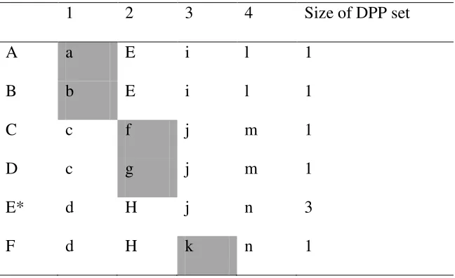
This leads us to measures based on dynamic principal parts. Consider Table 3, which is
INSERT TABLE 3 ABOUT HERE
Dynamic principal parts have the virtue of measuring what is required to infer the full
paradigm lexeme by lexeme. The number of cells in the principal parts set can differ for each
lexeme. The choice of paradigm cells can also differ. That is, there is no requirement for
lexemes to share cells in their principal parts set. In Table 3 lexemes of class A have one
dynamic principal part, and this is associated with the morphosyntatic property set 1. This is
also true for lexemes of class B. Lexemes of classes C and D, on the other hand, use one
dynamic principal part associated with morphosyntatic property set 2. Lexemes of class F
also require only one dynamic principal part, but this time associated with morphosyntactic
property set 3. For lexemes of class E, however, one MPS is insufficient to infer the full
paradigm. It turns out that the minimum size of the dynamic principal part set for class E is
three. There are three alternative analyses, equally optimal, and each involving
morphosyntactic property set 3: {3,1}, {3,2} or {3,4}. For Table 3 the average size of the
optimal dynamic principal parts set is 1.33 (8/6). This is an important measure of complexity:
(4) ‘The larger the size of an IC system’s optimal dynamic principal-part sets, the more
complex it is.’ (p. 330)
This measure is less brittle than (2), because it is sensitive to the variation across lexemes.
Intuitively, the greater on average the size of the dynamic principal-part set, the more burden
has to be taken on by listing information, rather that inferring things by rule. This makes the
system more complex. For the twelve case-study datasets looked at in MT Palantla Chinantec
(or Tlatepuzco Chinantec) has the highest average size of optimal dynamic principal-part sets
(p. 332), making it the most complex in this dimension. If we wish to understand (4) in terms
the size of the paradigm for which the DPP size is calculated. The Palantla Chinantec
paradigm in the dataset used for MT has twelve paradigm cells. So an average size of 1.33 is
still much less than half the paradigm, indicating that the rule system still does a lot. If the
average DPP size for a 12-cell paradigm were 6 or higher, then the role of the rule system
(inference) would be much less.
Given the size of the average dynamic principal parts analysis the next measure, I
suggest, can be interpreted as a way of understanding the consistency of the system. This is
the average ratio of actual to possible optimal dynamic principal-parts analyses (cf. (3), the
density measure used for static principal parts). Stump & Finkel say the following:
(5) ‘The smaller the average ratio of actual to possible optimal dynamic principal-parts
analyses for an IC system, the more complex it is.’ (p. 330)
Consider the optimal dynamic principal-part sets in Table 3. For the sake of illustration, let’s
assume that the lexicon consists of six lexemes, each representing one of the six classes in
Table 3. The ratio is calculated for each lexeme by dividing the number of actual optimal
dynamic principal-part analyses by the number of possible ones. For lexeme A (belong to
class A), there is one optimal dynamic principal part. The number of possible (as opposed to
actual) optimal dynamic principal parts of size one in a four-cell paradigm is four. The ratio
of actual to possible optimal dynamic principal-part analyses for lexeme A is therefore 25%
(1/4). It can easily be confirmed that it is also 25% for A, B, C, D and F. For lexeme E
(representing class E), as we have seen, there actually exist three optimal dynamic
principal-part analyses of size two. The possible (as opposed to actual) number of optimal dynamic
principal-part analyses of size two in a four-cell paradigm is six, because there are six ways
of choosing two from four. The ratio of actual to possible optimal dynamic principal-part
analyses for lexeme E is therefore 50% (3/6). The average ratio of actual to possible optimal
ratios for the set of lexemes, namely 29.2% (Table 4). (The three analyses for lexeme E are
presented on separate rows.)
INSERT TABLE 4 ABOUT HERE
Intuitively, the average ratio of actual to possible optimal dynamic principal-parts analyses
provides us with a measure of how the work is divided up between the different elements of
the system. Although this view is not explicitly stated or endorsed in MT, as far as I could
see, one way we could understand the average ratio of actual to possible optimal dynamic
principal-parts is as a proxy measure of the relationship between rules and listing. Let’s
consider the size-two analyses in Table 4, associated with class E, and construct a system
based on rules and listed items (or sets of items). We also constrain this system by stating that
only items (or sets of items) that are capable of predicting the whole paradigm can appear on
the left-hand side of a rule. The actual system of three combinations Table 4 uses all four
MPS: 1, 2, 3, 4. Bearing in mind the constraint that says we can only allow items that predict
the whole paradigm on the left-hand side, we have the following six rules:
{1,3} 2
{1,3} 4
{2,3} 1
{2,3} 4
{3,4} 1
The first of these rules says that the MPS 1 and MPS 3 combined predict MPS 2, and so on.
For class E in Table 4 we therefore have four items that can be listed (all four MPS) and six
rules.
If we imagine, contra Table 4, that for class E there is only one analysis of size two that
works. Let’s say {1,3}, although it does not matter which. Under this hypothetical system we
would need the following rules:
{1,3} 2
{1,3} 4
We now have two MPS that are listed, and two rules. In a certain sense this would be a
system for class E where the rules and the listing are in balance. How does this relate to the
ratio of actual to possible optimal dynamic principal-parts? This would be the system where
there is only one analysis of size two, and the ratio of actual to possible optimal dynamic
principal-parts for class E would be as low as it could be, namely 17% (1/6). According to
(5), this is complex because it inhibits reliable inferences. Alternatively, we might construe
the ratio as a measure of a different notion of morphological complexity, one in which lexical
listing and the rule system are in balance. This will be at its highest (and the ratio therefore at
its lowest), with no alternative analyses of that size, when half the paradigm is listed (that is,
the size of the average dynamic principal parts set is equal to half the paradigm) and
consequently there will be an equal number of rules that predict each of the remaining cells in
the other half of the paradigm. If the size of the dynamic principal-part set is less than half the
paradigm, rules, while if it is greater than half the paradigm size, listing dominates.
Moving from the predictive power of combinations of cells Stump & Finkel present the
(6) ‘The higher an IC system’s cell predictor number (averaged across ICs), the more
complex it is.’ (p. 332)
The cell predictor number is averaged across an inflectional class. It tells us on average how
many principal parts are required to predict a cell within the inflectional class. When
averaged across all inflectional classes, it tells us how predictable the average paradigm cell
is. This measure tells us something about the strength of the rule system within the language,
as does the next one, average cell predictiveness.
In MT the average predictiveness of a cell can be quantified:
(7) ‘The lower an IC system’s average cell predictiveness, the more complex it is.’ (p.
332)
Naturally, the lower number here gives the more complex result, as a stronger rule system
will make a cell more predictive of another cell. The utility of these measures is that they try
to move down to the individual cell level. One of the things we have insufficient knowledge
about is what contributes to elements of the paradigm coming together to be part of an
effective principal part combination. Some cells may be very effective at picking out
sub-elements of the paradigm and contributing this to principal parts. But understanding the
extent of typological difference between paradigm elements based on the extent of their
predictability and predictiveness is an under-researched area, and these measures are very
valuable for taking this forward.
In MT it is noted that average IC predictability is also a dimension where there can be
significant variation across languages:
(8) ‘The lower an IC system’s average IC predictability, the more complex it is.’ (p. 334)
IC predictability for a given inflectional class is essentially the ratio of adequate dynamic
principal parts sets to all non-empty subsets of cells belonging to that class. It is therefore an
the inflectional class in question. This can be calculated for each inflectional class and
averaged over the whole system (‘average IC predictability’). Where all possible
combinations of cells would work, then the average IC predictability would be high. As we
see in section 3, MT predicts that inflectional classes with low type frequency (‘marginal
classes’) also have a more detrimental effect on the IC predictability of a more central class
(that is, one that contains lots of types) than central classes have on the IC predictability of
marginal classes. The statement in (8) is therefore useful for formulating what appears to be a
strong generalization about inflectional classes.
The next measure deals with individual cells, so that we can make a contrast between
predicting cells and predicting whole ICs.
(9) ‘The lower an IC system’s average cell predictability, the more complex it is.’ (p. 314)
Average cell predictability does not care about inflectional classes as such. For a specific cell
in the paradigm it is an expression of a paradigm’s subsets of distillations that predict that
cell as a proportion of all subsets. This can then be average across the lexicon. A high cell
predictability is therefore an indication that the system can be effectively described by
(implicational) rules. This is why low cell predictability is associated with complexity in the
sense that it inhibits reliable inferences.
The final measure for the ten correlates of morphological complexity is the n-MPS
entropy measure. This measure computes the entropy of a given cell based on a combination
of other cells, normally set to four (that is, combinations of size 4 or less).
(10) ‘The higher an IC system’s average n-MPS entropy, the more complex it is.’ (p. 337)
This could therefore be construed as an information-theoretic version of cell-predictability.
Stump & Finkel express the view that morphological complexity cannot be reduced to a
It may be reasonable to highlight certain of these measures as being of more interest
than others, and some of these are used in key predictions, to which we now turn. Naturally,
given the scope and the book, I am not able to address all of the predictions, but concentrate
on those that appear to me of particular interest.
3. Some key predictions
An important observation is made in MT about the relationship between the average cell
predictor number and average number of dynamic principal parts. Recall that the average cell
predictor number tells us how many principal parts on average are required to determine a
paradigm cell. This is different from the average dynamic principal part number, which gives
us the average number of dynamic principal parts required to predict the whole paradigm. In
Chapter Three of MT ten languages are compared in terms of the average cell predictor
number and the dynamic principal-part number. For each of the languages compared the
average cell predictor number is either equal to or smaller than the dynamic-principal part
number. Stump & Finkel note that this suggests that the Low Entropy Conjecture (Ackerman
& Malouf 2013) can be further refined (p. 61): ‘the determination of a given realized cell
involves lower expected conditional entropy than the determination of the full paradigm to
which it belongs.’ Indeed, a key benefit of the work presented in MT is that it allows us to
tease apart properties of morphological complexity associated with cells from those
associated with whole inflectional classes, for which there are also predictions to be made.
In contrast, an important prediction in relation to inflectional classes is the Marginal
Detraction Hypothesis, introduced in Chapter Eight:
(11) ‘Marginal ICs tend to detract most strongly from the IC predictability of other ICs.’ (p.
225)
Marginal inflectional classes are defined in terms of type frequency (p. 225), not token
lexemes. Recall that IC predictability expresses the number of adequate dynamic principal
part analyses as a fraction of all possible dynamic principal part analyses. Maximum IC
predictability (that is, of value 1) means that the number of adequate principal part analyses is
the same as the potential number. The key idea is that marginal inflectional classes will
detract more from IC predictability of central classes, than central classes will detract from IC
predictability of marginal classes. In MT this is illustrated by using an English-like example
containing a maximum of four ICs, based on ablaut series, as illustrated in Table 5, where the
most marginal class contains only one lexeme, namely the verb run.
INSERT TABLE 5 ABOUT HERE
The last column has been added here in order to illustrate what the Marginal Detraction
Hypothesis says. In the example in Table 5 there are three morpho-syntactic properties
(present, past, past participle). There are seven non-empty members of the powerset of {pres,
past, past_part}:
{past ptcp}
{past}
{present}
{past ptcp, present}
{past, past ptcp}
{past, present}
{past, past ptcp, present}
The penultimate column shows us the IC predictability of conjugation class (a), more
marginal classes are progressively added. For (a) on its own (that is, without any other
powerset will trivially predict the IC. When we add class (b) the IC predictability of (a)
reduces to 0.571, because we need to know the past tense form in order to predict the class,
and four of the seven non-empty members of the powerset contain this information. The
smaller class (c) detracts further from the IC predictability of (a), as we need to know both
the past and the past participle (that is, two out of the seven non-empty members of the
powerset). For class (d) we need to know all three of the properties, and therefore only one
out of the seven non-empty members of the powerset will work.
The final column, which is not given in MT, calculates the IC predictability of the most
marginal class (d), depending on the presence of the other ICs, progressing through the
marginal ones to the central ones. That is, we carry out the exercise in exactly the reverse
order. When only class (d) is given the IC predictability is 1.000. When we add class (c) the
IC predictability for (d) decreases to 0.857, because we need to know either the present or the
past participle, so that six out of the seven non-empty members of the powerset work. Adding
class (b) reduces the IC predictability of (d) further to 0.714, because only five out of seven
non-empty members of the powerset are predictive (that is, {present} plus the other four sets
that contain two or more properties). Finally, adding class (a) reduces the IC predictability of
(d) down to 0.571, because only four out of seven non-empty members of the powerset are
predictive (namely {present}, {past ptcp, present}, {past, present} and {past, past ptcp,
present}). This exercise requires us to force the number of distillations to remain the same
when we make the comparison, as it is noted in MT that where adding an IC increases the
number of distillations this can increase the predictability. (For the purposes of the
calculations in Table 5 we have forced the number of distillations to remain at three.)
It should be apparent from looking at Table 5 that addition of marginal classes detracts
more from the measure of IC predictability for central classes than the addition of central
we start with the central class (a), by the time we get to class (d), IC predictability for (a) has
deteriorated to 0.143. In contrast, if we start with the marginal class (d), by the time we get to
class (a), IC predictability has deteriorated only to 0.571. In MT detailed examples from both
Icelandic and French are used to support the Marginal Detraction Hypothesis.
We should consider what is required for a class to detract from the IC predictability of
another class. Note that a key difference in Table 5 between the ICs is that the central class
contains three allomorphs, whereas the other three have two allomorphs, each of which is
shared with the central class. If a class does not share allomorphs with another class it will
not detract from it. Presented with an inflectional class in which there is overlap between
allomorphs, the Marginal Detraction Hypothesis should allow us to predict which has higher
type frequency.
4. Representational issues
An important issue that arises from MT, and one that is dealt with in depth by the authors is
the question of representation. In the chapter on speaker-oriented and hearer-oriented plats, it
is shown that significant differences in results can depend on the nature of the representation.
The addition of gender information (that is, information about the associated gender
agreement patterns) can diminish IC complexity. Gender appears to be useful in increasing
both predictability and predictiveness, while delimitation of stems increases predictiveness,
but not predictability.
Another important question is the distinction that is made in MT between exponence
and exponents (p. 21), where the former refers to the realization of the complete
morphosyntactic specification associated with a word form, while the latter refers to elements
related to part of the morphosyntactic specification. This brings with it the interesting
realization, something that the tools provided by MT may put us in a position to answer in the
long run.
The representational issues are big ones, of course, but they also create potential for
new research programmes in which we consider the relative importance of exponents as
predictors, as opposed to being predictable. One thing that would be useful to know, for
instance, is how, if at all, the notion of default fits into the picture. This is an important issue,
because we can see other forms as being predictive of defaults, or we can see that defaults are
predictable. It is hard to know how substantial this issue may be, but it is worth investigating.
In fact, with MT there are many ideas that represent key directions for the future, should we
wish to take them up, and it is to some of these that I now turn.
5. Key ideas and future direction for the field
An important distinction is made in MT between two types of rule. One type of rule specifies
the realization, taking a stem and a morpho-syntactic property set. An alternative type are
implicative rules that deduce one cell of a paradigm on the basis of one or more other
paradigm cells. Indeed, MT provides a hybrid conception of inflectional morphology that
makes use of W-relations and R-relations (Chapter Nine). The value of rule systems that
work with multiple elements of the paradigm is also something that is recognized within
contemporary NLP work (see Kann, Cotterell & Schütze 2017). As Sims & Parker (2016)
note, there is significant typological variation in the extent to which implicative relations play
a role in different morphologically complex systems. Sims & Parker’s work considers the
contributions of type frequency and implicative to speakers’ knowledge. In the hybrid model
provided in MT two systems are contrasted: One in which the rule system can make use of IC
diacritics (that is, a purely morphological feature) and one in which implicative rules can be
used. If the role of implicative relations is a matter of typological variation, then the hybrid
As noted, the fundamental starting point is that morphological complexity is about how
readily reliable inferences can be made about realization. Inference is naturally associated
with rules, and MT talks of maximally transparent and maximally opaque ICs (p. 81). In a
maximally transparent system each cell of the IC predicts every other cell (see also Baerman,
Brown & Corbett 2017: 101-2 on grid systems). In a maximally opaque system no
combination of paradigm cells can predict the other members of the paradigm. In terms of
inference the latter is considered morphologically complex, while the other is the opposite.
The two maximal systems (transparent and opaque) presented in MT could also be
understood in terms of rules and lexical listing. The maximally transparent system can be
described by an effective system of implicational rules, where each cell predicts every other
cell. The maximally opaque system requires listing of all forms for the given class. If the
Low Conditional Entropy Conjecture (Ackerman & Malouf 2013) is correct, the maximally
opaque system will not be found. So it is worth considering where we should be focusing our
efforts as morphologists, if one of the extremes is not likely to be attested (which is an
important finding, if correct). Returning to the two basic types identified in MT we can also
note that they represent two ‘pure’ systems: One is based PURELY on rules, while the other
would be based PURELY on listing (the high entropy end). As we know, virtually all
morphology involves an interplay of lexical stipulation (listing) on the one hand, and rules on
the other. We could therefore consider this interplay itself to be a type of complexity (called
‘central system complexity’ in Baerman, Brown & Corbett 2017), which should be at its
highest when the rule system and the system of listing are involved in equal measure.4 From
this perspective maximally transparent and maximally opaque systems are both simple: They
do not involve any compromise between rules and listing, as they are either purely one or the
other. What is more, for one of the measures in MT they both have the same value. That is,
the plat illustrating the maximally opaque system on p. 83 of MT the ratio is 100% because
for every class all three distillations are required, and therefore for every class the number of
possible dynamic principal part analyses is the same as the number of actual analyses (one).
This value for the maximally transparent system is also 100%, because this reduces down to
one distillation, and therefore one analysis. This suggests that the average ratio of actual to
possible optimal dynamic principal-parts could play an important role in investigating this
particular type of complexity.
6. Conclusion
MT provides interesting predictions about what is possible in morphologically complex
systems, as we see with the Marginal Detraction Hypothesis, for instance, and a range of
different measures that pick out subtly different aspects of IC systems. As with any
ground-breaking work it demands a lot of attention when reading, and also prompts thoughts about
the possible implications of the measures provided. Some may prove to be more valuable
than others. In particular, it is reasonable to assume that the measures associated with
dynamic principal parts will prove particularly useful, because they can provide a realistic
assessment of what needs to be stored and what can be inferred, without imposing a rigid
threshold for all items in the lexicon. Perhaps MT’s biggest service is to provide the field
with a new set of measures specifically tailored for morphological complexity. As a toolkit
for measuring the complexity of IC systems MT should be the first port of call. Stump &
Finkel note that there is reason to be skeptical that the different measures can be reduced
down to one, which would indicate that we cannot expect a simple account of the
morphologically complex in the near future. But if such an account were to exist it would
require a thorough understanding of the full range of typological variation that MT now
allows us to measure.
Ackerman, Farrell, James P. Blevins & Robert Malouf 2009. Parts and wholes: Patterns of
relatedness in complex morphological systems and why they matter. In James P.
Blevins & Juliette Blevins (ed.), Analogy in grammar: Form and acquisition. Oxford:
Oxford University Press. 54-82.
Ackerman, Farrell & Robert Malouf 2013. Morphological organization: The low conditional
entropy conjecture. Language. 89: 429-464.
Baerman, Matthew, Dunstan Brown & Greville G. Corbett. 2005. The syntax-morphology
interface: A study of syncretism. Cambridge: Cambridge University Press.
Baerman, Matthew, Dunstan Brown & Greville G. Corbett. 2017. Morphological complexity.
Cambridge: Cambridge University Press.
Bane, Max 2008. Quantifying and measuring morphological complexity. In Charles B. Chang
& Hannah J. Haynie (eds.), Proceedings of the 26th West Coast Conference on Formal
Linguistics. Somerville MA: Cascadilla Proceedings Project. 69-76
Dahl, Östen 2014. Review of Gregory Stump & Raphael A. Finkel, Morphological Typology:
From Word to Paradigm (Cambridge Studies in Linguistics 138). Cambridge:
Cambridge University Press, 2013. Pp. Xxiv + 402. Nordic Journal of Linguistics
37(1): 126-132.
Kann, Katharina, Ryan Cotterell & Hinrich Schütze 2017. Neural multi-sourcemorphological
reinflection. In Proceedings of the European Chapter of the Association for
Computational Linguistics, Valencia 3-7 April.
Sims, Andrea D. & Jeff Parker 2016. How inflection class systems work: On the
informativity of implicative structure. Word Structure, 9: 215-239.
Author’s address: (Dunstan Brown)
Department of Language and Linguistic Science
Heslington, York
YO10 5DD
United Kingdom
Table 1. Burmeso verbal forms (Donohue 2001: 100, 102)
SG I PL I SG II PL II SG III PL III SG IV PL IV SG V PL V SG VI PL VI
‘see’ j- s- g s- g- j- j- j- j- g- g- g-
Table 2. Small static principal parts sets are very likely to have higher density
Size of Static Principal Parts Set Number of Alternative Analyses Actual for Density <0.001
1 21 0
2 210 0
3 1,330 0
4 5,985 2
5 20,349 6
6 54,264 16
7 116,280 34
8 203,490 60
9 293,930 86
10 352,716 104
11 352,716 104
12 293,930 86
13 203,490 60
14 116,280 34
15 54,264 16
16 20,349 6
17 5,985 2
18 1,330 0
19 210 0
20 21 0
Table 3. Dynamic principal parts
1 2 3 4 Size of DPP set
A a E i l 1
B b E i l 1
C c f j m 1
D c g j m 1
E* d H j n 3
Table 4. Calculating the average ratio of actual to possible optimal dynamic principal-parts
analyses for an IC system
1 2 3 4 Size Ratio
A a e i l 1 25% (1/4)
B b e i l 1 25% (1/4)
C c f j m 1 25% (1/4)
D c g j m 1 25% (1/4)
E* d h j n -- --
E* d h j n -- --
E* d h j n 3 50% (3/6)
F d h k n 1 25% (1/4)
Table 5. Marginal classes detract more than central classes (Stump & Finkel 2013: 226)
IC
Predictability
of (a), given
knowledge
of this IC
and ones
above.
IC
Predictability
of (d), given
knowledge
of this IC
and ones
below. Stem Vocalism
Present Past Past
Participle
Sample
Lexemes
(a) -ɪ- -æ- -ʌ- SING,
SINK,
SWIM
1.000 0.571
(b) -ɪ- -ʌ- -ʌ- CLING,
STICK, DIG
0.571 0.714
(c) -ɪ- -æ- -æ- SIT, SPIT 0.286 0.857
Notes
1 Syncretism is not relevant for defining a distillation. In order to belong to the same
distillation there is no requirement for the MPSs to share allomorphs (that is, to be syncretic,
as defined in Baerman, Brown & Corbett 2005, for instance). What is required is that across
MPSs belonging to the same distillation the same inflectional classes are distinguished. For
instance, the MPSs SG V and PL VI belong to the one distillation in Table 1, but they do not
share exponents.
2 This is the binomial co-efficient = !
! !, which in this case is therefore !
! ! .
3 The term ‘large’ is not entirely accurate here, because if the static principal parts set is
larger than half the paradigm size the number of possible analyses will start to reduce.
Informally at least we do not expect the static principal part set to require over half of the
cells in the paradigm to be given, and stick to this informal use of the term ‘large’.
4 It is worth pointing out here that the intention is not to oust one notion of complexity with
another, but merely to consider the different types of complexity and what they tell us.
Indeed, one of the great services of MT is that it provides us with the means of measuring