This is a repository copy of An improved expanding and shift scheme for the construction
of fourth-order difference co-arrays.
White Rose Research Online URL for this paper:
http://eprints.whiterose.ac.uk/134925/
Version: Accepted Version
Article:
Cai, J., Liu, W. orcid.org/0000-0003-2968-2888, Zong, R. et al. (1 more author) (2018) An
improved expanding and shift scheme for the construction of fourth-order difference
co-arrays. Signal Processing, 153. pp. 95-100. ISSN 0165-1684
https://doi.org/10.1016/j.sigpro.2018.06.025
Reuse
This article is distributed under the terms of the Creative Commons Attribution-NonCommercial-NoDerivs (CC BY-NC-ND) licence. This licence only allows you to download this work and share it with others as long as you credit the authors, but you can’t change the article in any way or use it commercially. More
information and the full terms of the licence here: https://creativecommons.org/licenses/
Takedown
If you consider content in White Rose Research Online to be in breach of UK law, please notify us by
An Improved Expanding and Shift Scheme for the
Construction of Fourth-Order Difference Co-Arrays
Jingjing Caia,∗, Wei Liub,∗∗, Ru Zonga, Bin Wua
a
Department of Electronic and Engineering, Xidian University, Xi’an, 710071, China b
Department of Electronic and Electrical Engineering, University of Sheffield, Sheffield, S1 4ET, United Kingdom
Abstract
An improved expanding and shift (IEAS) scheme for efficient fourth-order difference co-array construction is proposed. Similar to the previously pro-posed expanding and shift (EAS) scheme, it consists of two sparse sub-arrays, but one of them is modified and shifted according to a new rule. Examples are provided with the second sub-array being a two-level nested array (IEAS-NA), as such a choice can generate more fourth-order differ-ence lags (FODLs), although with the same number of consecutive lags. Furthermore, the array aperture of IEAS-NA is always greater than the corresponding EAS structure, which helps improving the DOA estimation result. Simulations results are provided to show the improved performance by the proposed new scheme.
Keywords: Sparse arrays, fourth-order difference co-array, expanding and shift scheme, cumulant.
1. Introduction
Sparse arrays combined with the second-order difference co-array con-cept can provide much more degrees of freedom (DOFs) than traditional uniform linear arrays (ULAs), and many methods have been proposed for underdetermined direction of arrival (DOA) estimation based on such arrays, such as the spatial smoothing-based subspace methods [1, 2], or compressive
∗Corresponding author: Tel.: +86-29-88204759; fax: +86-29-88204759. ∗∗Corresponding author: Tel.: +44-114-2225813; fax: +44-114-2225834.
sensing (CS)-based methods [3, 4, 5, 6, 7]. Two representative sparse array structures are the co-prime arrays (CPAs) [8, 3, 9] and the nested arrays (NAs) [10, 11, 12, 13, 14].
By exploiting additional statistical properties of the impinging signals, such as non-Gaussianity or non-stationarity, fourth-order difference co-arrays can be constructed for underdetermined DOA estimation with further in-creased DOFs [15, 16, 17, 18, 19, 20, 21, 22, 23]. Two of the sparse array con-struction methods specifically designed for fourth-order difference co-array generation are the extension based on CPAs and NAs in [23, 24], which we call the three sub-arrays (TSA) scheme in this paper, and the expanding and shift (EAS) scheme proposed in [25], which are based on modifying and combining two existing sparse array structures. It was shown that the EAS scheme can generate much more consecutive co-array virtual sensors than the TSA scheme.
In this work, we propose an improved version of the EAS scheme which can generate more DOFs with a lager aperture. Same as the EAS scheme, there are two sparse sub-arrays in the proposed improved EAS (IEAS) scheme: one of them is expanded and shifted, but the value of shift is con-cerned with the consecutiveness of the second sparse array. As an implemen-tation of the EAS scheme, the EAS-NA structure, where the second sparse sub-array is based on the nested array, is the most efficient one, generating more consecutive fourth-order difference lags (FODLs) than the others [25]. Similarly, one implementation of the IEAS scheme is the IEAS-NA struc-ture, where the second sparse sub-array is derived from a nested array, and is more efficient than the others. The number of consecutive FODLs for both EAS-NA and IEAS-NA is exactly the same, while the number of total FODLs of IEAS-NA is greater than that of EAS-NA. More importantly, the sensors of IEAS-NA are distributed in a wider range than EAS-NA, lead-ing to a lager array aperture. These advantages result in a better DOA estimation performance compared to the original EAS-NA scheme.
This paper is organized as follows. The EAS scheme is reviewed in Sec. 2 and the proposed IEAS scheme is introduced in Sec. 3. Design examples and a comparison of different schemes are presented in Sec. 4. Simulation results are provided in Sec. 5 and conclusions are drawn in Sec. 6.
2. Review of The EAS Scheme
Ă 0
Ă 0
1
p d p d2 p dI
1I
p d p2Id pJ Id
[image:4.612.214.396.124.218.2]k
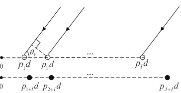
Figure 1: A sparse array structure consists of two sparse sub-arrays.
sensors as shown in Fig. 1. Denote the unit spacing by d, with d = λ/2. Then, positions of the whole array can be represented by a combination of the following two sets
P1={p1·d, p2·d, . . . , pI ·d}
P2={p1+I ·d, p2+I ·d, . . . , pJ+I·d}
(1)
Suppose there are K far-field independent non-Gaussian narrowband signals sk(t)(k = 1, . . . , K) impinging on the array. With the DOA of the
kth source being θk, and taking the origin “0” as the zero-phase reference point, the observed signalxi(t) at theith sensor is given by
xi(t) = K
X
k=1
exp(j2πpidcosθk/λ)sk(t) +ni(t) (2)
i= 1, . . . , I+J, whereni(t) is the additive Gaussian noise of theith sensor, independent of the signals. Suppose 1≤i, j, u, v≤I+J and{i, j, u, v} ∈Z. The fourth-order cumulant valueC(i,−j, u,−v) of theith,jth,uth andvth sensor observed signals can be expressed as [15]
C(i,−j, u,−v) =cum[xi(t), x∗
j(t), xu(t), x∗v(t)]
= K
X
k=1
exp[j2π(pi−pj+pu−pv)dcosθk/λ]·
cum(sk(t), s∗k(t), sk(t), s∗k(t))
(3)
The FODL expression (pi−pj+pu−pv) corresponding to the new virtual sensors can be written as
pi−pj+pu−pv = (pi−pj) + (pu−pv) (4)
Clearly, this FODL expression can be seen as two second-order difference lags added together and we could construct the fourth-order difference co-array by two separate second-order difference co-co-arrays with different ranges as shown in the EAS scheme [25], where we first expand the spacing of the second sparse array, and then shift the expanded array by a proper distance. For the EAS scheme, we assume two sparse arrays, which contains ¯M
and ¯N sensors, separately. They can be represented as
¯
Q1 ={q¯1·d,q¯2·d, . . . ,q¯m·d, . . . ,q¯M¯ ·d} ¯
Q2 ={q¯1+ ¯M·d,q¯2+ ¯M ·d, . . . ,q¯n+ ¯M ·d, . . . ,q¯N+ ¯¯ M ·d},
(5)
and the number of consecutive second-order difference co-array sensors for these two sub-arrays are defined as CM¯ and CN¯, separately.
To constructP1 andP2 according to the EAS scheme using the elements of ¯Q1and ¯Q2, ¯Q1 can be used asP1directly, but ¯Q2should be expanded and shifted to beP2. To be specific, the unit spacing of ¯Q2 should be expanded toCM¯ ·dat first, and then shifted by a proper distance ∆q, by which one sensor of the two sub-arrays will be co-located, so that one of the co-located sensors can be removed. To obtain a lager aperture, the last sensor of the first sub-array can coincide with the first sensor of the second sub-array. The number of physical sensors is thenI = ¯M forP1 andJ = ¯N−1 forP2, and the elements of the EAS scheme can be defined as
pi= ¯qm i= 1, . . . , I;m= 1, . . . ,M¯
pj = ¯qn+ ¯M ·CM¯ +∆q j= 1, . . . , J;n= 2, . . . ,N¯
(6)
where ∆q = ¯qM¯ −q¯1+ ¯MCM¯, and ¯q2+ ¯M ·CM¯ +∆q is the first sensor of P2. Note that the first sensor ¯q1+ ¯M ·CM¯ +∆q of P2 is co-located with ¯qM¯ and has been removed. As a result, the total number of sensors and FODLs of this scheme can be expressed as
¯
L= ¯M+ ¯N −1, CL¯ =CM¯CN¯ (7)
Define EAS-NA as the EAS scheme with the second sparse sub-array being a nested array. For a nested array, we have the property of ¯qN+ ¯¯ M − ¯
q1+ ¯M = CN¯−1
2 , where CN¯−1
second-order lags. For such a choice, an extra segment of 2(¯qM¯ −q¯1) con-secutive FODLs will be generated. Then, the EAS-NA structure can finally generate a number of consecutive FODLs as
CLna¯ =CM¯CN¯ + 2(¯qM¯ −q¯1). (8)
For the EAS-NA scheme, the number of total FODLs including consec-utive and nonconsecconsec-utive ones, is the same as the number of consecconsec-utive FODLs, which is given by
CT na¯ =CM¯CN¯ + 2(¯qM¯ −q¯1) (9)
3. The Improved EAS (IEAS) Scheme
Compared to the EAS scheme, instead of shifting the second sub-array in such a way that the two sub-arrays have one pair of co-located sensors, the IEAS scheme shifts the second sub-array further away from the first one and there are no co-located sensors in the new structure. Define IEAS-NA as the class of IEAS schemes with the second sparse sub-array being a nested array. As shown later, this further shift will increase the total FODLs of the IEAS-NA. Moreover, the aperture of the IEAS-NA scheme is increased which helps improve the resolution of the whole system.
Assume there are two sparse arrays which contains M and N sensors, separately, as given below.
Q1 ={q1·d, q2·d, . . . , qm·d, . . . , qM ·d}
Q2 ={q1+M ·d, q2+M ·d, . . . , qn+M ·d, . . . , qN+M ·d}
(10)
Assume these two sub-arrays can generate CM and CN second-order differ-ence lags, separately. The first step in IEAS is also expanding the second sparse array as in the EAS scheme, which can generate a consecutive inte-gers segment from−(CMCN −1)/2 to (CMCN −1)/2. Assuming the shift distance now is denoted by ∆s·d, the elements of IEAS sub-arrays with
I =M and J =N physical sensors can be represented by
pi =qm i= 1, . . . , I;m= 1, . . . , M
pj =qn+M ·CM +∆s j= 1, . . . , J;n= 1, . . . , N
(11)
Note that the FODLs generated by these two sub-arrays can be at least
increase the number of FODLs, and we can also use other strategies, such as choosingpi,pjandpvfromP1whilepufromP2. With this choice, using (pi−
pj) + (−pv) will generate consecutive integers by shifting the autocovariance of P1 to every negative points of P1. The consecutive integers segment generated by the autocovariance ofP1 is from−(CM −1)/2 to (CM−1)/2 with 0 at its center. Then, the consecutive integers segment shifted to−qM will be from −qM −(CM −1)/2 to−qM + (CM −1)/2, while the segment shifted to −q1 is from −q1−(CM −1)/2 to−q1+ (CM −1)/2. Removing the overlapped integers between these two segments, the overall consecutive integers segment is from−qM−(CM−1)/2 to−q1+(CM−1)/2 with 0 at its center. Then, the corresponding FODLs the combination [(pi−pj)+(−pv)]+
pugenerates can be considered as the consecutive integers segment generated by (pi−pj)+(−pv) being shifted again with the elements ofQ2at its center. Assuming fromqU+M toqV+M is the maximum consecutive integer range in
Q2, they can definitely generate consecutive FODLs from (qU+MCM+∆s)−
qM −(CM−1)/2 to (qV+MCM +∆s)−q1+ (CM −1)/2. To maximize the segment of FODLs, we would like the first point of this consecutive FODLs segment to be next to the last point of the consecutive FODLs segment
CMCN. In this case, the corresponding ∆s can be calculated as
qU+MCM +∆s−qM −(CM −1)/2 = (CMCN −1)/2 + 1, →
∆s= (CMCN −1)/2−qU+MCM + (CM −1)/2 +qM + 1.
(12)
With this value of ∆s, the maximum positive FODLs will be increased to (V −U+ 1)CM+qM−q1−1 and the overall consecutive FODLs will also increase accordingly. The total number of sensors and consecutive FODLs of this scheme can be expressed as
L=M +N
CL=CMCN + 2(V −U+ 1)CM + 2(qM −q1)
(13)
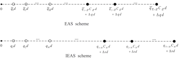
The physical layout of these two schemes is shown in Fig. 2, and the way of constructing the IEAS scheme is summarised in Tab. 1. The steps of constructing the EAS scheme is a little different, which only uses the steps 1, 2, 5, 6 and 7. The EAS scheme can remove one co-located sensor of the two sub-arrays by the shifting, while the IEAS scheme can generate more FODLs using the consecutiveness of the second sub-array.
Ă Ă
Ă
1
q d q d2 q dM 1 +
! M M
q C d
q d
2 +
!
M M
q C d
q d
N + !
M M
q C d
q d
EAS scheme
Ă Ă Ă
IEAS scheme 1
q d q d2 q dM 2
! M M
q C d
sd !
N M M
q C d
sd 1
!
M M
q C d sd
0
[image:8.612.134.479.129.240.2]0
Figure 2: The physical layout of the EAS and IEAS schemes.
Table 1: Steps of the IEAS scheme
step 1 Calculate the second-order difference lags of Q1 asCM step 2 Expand the inter-element of Q2 toCM ·d
step 3 Calculate the second-order difference lags of Q2 asCN step 4 Count the consecutive sensors of Q2 as (V −U + 1) step 5 Obtain the last sensor position pM ofQ1
step 6 Calculate the shift value of ∆s
step 7 Shift Q2 to∆s
contains the best consecutiveness in itself. It can be derived that the IEAS-NA can generate the most FODLs among all possible IEAS implementations based on existing sparse array structures. Let N1 and N2 be the two pa-rameters of the second sparse array, and the maximum consecutive range of integers in the nested array is from 1 to (N1+ 1) with (N1+ 1) sensors in it, which meansV −U+ 1 =N1+ 1, so that the number of consecutive FODLs is given by
CLna=CMCN + 2(N1+ 1)CM + 2(qM −q1) (14) Then, we can also derive the total number of FODLs of the IEAS-NA. For IEAS-NA, the consecutive FODLs correspond to theN1+ 1 consecutive sensors of the second sparse array, and the total number of FODLs should also depend on the remaining (N2−1) nonconsecutive sensors of the second array. Assume in (pi−pj) + (pu−pv),pi, pj andpv are chosen fromQ1while
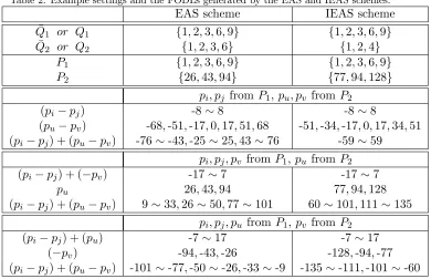
Table 2: Example settings and the FODLs generated by the EAS and IEAS schemes.
EAS scheme IEAS scheme
¯
Q1 or Q1 {1,2,3,6,9} {1,2,3,6,9} ¯
Q2 or Q2 {1,2,3,6} {1,2,4}
P1 {1,2,3,6,9} {1,2,3,6,9}
P2 {26,43,94} {77,94,128}
pi, pj from P1,pu, pv from P2
(pi−pj) -8∼8 -8∼8
(pu−pv) -68,-51,-17,0,17,51,68 -51,-34,-17,0,17,34,51 (pi−pj) + (pu−pv) -76∼-43,-25∼25,43∼76 -59∼59
pi, pj, pv from P1,pu from P2 (pi−pj) + (−pv) -17∼7 -17∼7
pu 26,43,94 77,94,128 (pi−pj) + (pu−pv) 9∼33,26∼50,77∼101 60∼101,111∼135
pi, pj, pu from P1,pv from P2 (pi−pj) + (pu) -7∼17 -7∼17
(−pv) -94,-43,-26 -128,-94,-77 (pi−pj) + (pu−pv) -101∼-77,-50∼-26,-33∼-9 -135∼-111,-101∼-60
it. Considering the negative lags, the total FODLs generated by theN2−1 nonconsecutive sensors of the second array should be (N2 −1)(3CM −1). That means the total FODLs of the IEAS-NA scheme is given by
CT na=CMCN + 2(N1+ 1)CM + 2(qM −q1) + (N2−1)(3CM −1)
(15)
Now an example for both the EAS-NA and IEAS-NA schemes is pro-vided, with the settings and generated FODLs listed in Tab. 2. The total number of sensors is ¯L = L = 8, and the shift value ∆s = 25 for EAS-NA and ∆q = 60 for IEAS-NA. It can be seen that the EAS-NA scheme generatesCL¯ = 203 andCT¯ = 203 FODLs, while the IEAS-NA scheme gen-eratesCL= 203 and CT = 253 FODLs. The nonconsecutive FODLs of the IEAS scheme are in one positive segment from 111 to 135 and one negative segment from−135 to−111 with 25 lags in each of them.
4. Comparisons between IEAS-NA and EAS-NA
the same number of physical sensors, we can have different sub-array pa-rameters, which then results into different number of consecutive FODLs for the different schemes. To have a fair comparison, we choose the parameters giving the maximum number for each scheme, and compare the number of consecutive FODLs and total FODLs.
For IEAS-NA, the first sub-array contains M sensors while the second one contains N sensors; in EAS-NA, because the first sensor of the second sub-array is also the last sensor of the first sub-array, the number of sensors for the two sub-arrays is denoted by ¯M and ¯N−1, separately. Let ¯N1 and
¯
N2 denote the two parameters of the second sub-array in the EAS scheme. We have ¯N1 + ¯N2 = ¯N and for IEAS-NA, N1+N2 = N. Then, the total number of sensors can be written as
¯
L= ¯M+ ¯N1+ ¯N2−1, L=M+N1+N2 (16) for EAS-NA and IEAS-NA, respectively; the number of consecutive FODLs
CL¯ and CL can be rewritten as
CLna¯ =CM¯(2 ¯N1N¯2+ 2 ¯N2−1) + 2(¯qM¯ −q¯1)
CLna=CM(2N1N2+ 2N2+ 2N1+ 1) + 2(qM −q1)
(17)
The maximum value of CL¯ depends on the distribution of ¯M, ¯N1 and ¯
N2, while CL depends on the distribution of M, N1 and N2 for CL. Note that the structures of CLna¯ and CLna in (17) are almost the same. If we assume ¯L=L, ¯M =M andCM¯ =CM, and with the assumptionN1+N2 =
¯
N1+ ¯N2−1 =N, we next give a comparison between CLna¯ and CLna. WhenN1+N2 =N is odd, ¯N1+ ¯N2 =N+ 1 is even, vice versa. To get the maximum number of second-order difference lags for a nested array, the parameter settings should be
(¯
N1 = ¯N2 = (N+ 1)/2 N is odd ¯
N1 =N/2,N¯2=N/2 + 1 N is even
(
N1 = (N−1)/2, N2= (N + 1)/2 N is odd
N1 =N2 =N/2 N is even
(18)
Interestingly, with this setting the maximum value of CLna¯ and CLna will be exactly the same, given by
CLmax=CLmax¯ =
CM[(N2+ 1)/2 + 2N] + 2(qM −q1)
N is odd
CM(N2/2 + 2N+ 1) + 2(qM −q1)
N is even
We can finally draw the conclusion that, when the total number of sensors for the EAS-NA and the IEAS-NA is the same, they can obtain the same number of consecutive FODLs.
In the same way, define CT max¯ and CT max as the maximum of CT na¯ andCT na, separately. BecauseCT na¯ equals CLna¯ , the settings ofCLmax¯ are suitable for CT max¯ . While CLna is contained in CT na and also the main part ofCT na, the settings of CLmax are also suitable for CT max. These two maximum values can be given by
CT max¯ =
CM[(N2+ 1)/2 + 2N] + 2(qM −q1)
N is odd CM(N2/2 + 2N + 1) + 2(qM −q1)
N is even
CT max =
CM[(N2+ 1)/2 + 2N] + 2(qM −q1) + (N−1)(3CM−1)/2 N is odd
CM(N2/2 + 2N + 1) + 2(qM −q1)
+ (N−2)(3CM−1)/2 N is even
(20)
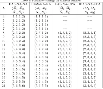
Let the first sub-array of the IEAS-NA and EAS-NA schemes as the nested array (NA) and co-prime array (CPA), the resultant schemes are referred to as INA, NA, ICPA and EAS-NA-CPA, separately. We useM1andM2as the two parameters of the first sparse array for IEAS-NA, while ¯M1 and ¯M2 for EAS-NA. The parameter settings are listed in Tab. 3, which are chosen to give the maximum number of FODLs for each scheme, while the maximum number of consecutive FODLs and total FODLs are shown in Fig. 3.
Furthermore, the sensors of INA are set in a wider range than EAS-NA. The last sensor location of these two schemes can also be derived as
qL¯ = ( ¯N1N¯2+ ¯N2−1)CM¯ + ¯qM¯
qL = (2N1N2+ 2N2−1)CM +qM (21)
Their maximum values are
qLmax¯ =
(
CM[(N2−1)/4 +N] +qM N is odd
CM(N2/4 +N) +qM N is even
qLmax=
(
CM[(N2−1)/2 +N] +qM N is odd
CM(N2/2 +N−1) +qM N is even
Table 3: Parameter settings for different schemes.
EAS-NA-NA IEAS-NA-NA EAS-NA-CPA IEAS-NA-CPA
L ( ¯M1,M¯2, (M1, M2, ( ¯M1,M¯2, (M1, M2, ¯
4 6 8 10 12 14 16 18 20 500
1000 1500 2000 2500 3000 3500 4000 4500 5000 5500
Number of sensors
Number of FODLs
CL of EAS−NA−NA,IEAS−NA−NA CT of EAS−NA−NA
CL of EAS−NA−CPA,IEAS−NA−CPA CT of IEAS−NA−NA
[image:13.612.216.394.131.272.2]CT of EAS−NA−CPA CT of IEAS−NA−CPA
Figure 3: Number of FODLs with respect to the number of sensors.
4 6 8 10 12 14 16 18 20
500 1000 1500 2000 2500 3000 3500 4000
Number of sensors
Last sensor locations
qL of EAS−NA−NA qL of IEAS−NA−NA qL of EAS−NA−CPA qL of IEAS−NA−CPA
Figure 4: Last sensor position with respect to the number of sensors.
With the same setting as in Tab. 3, the values ofqL¯ andqLare shown in Fig. 4. From Figs. 3 and 4, we can see that the consecutive FODLs of IEAS-NA is always equal to that of EAS-IEAS-NA, and the total FODLs of IEAS-IEAS-NA is always greater than that of EAS-NA. Moreover, IEAS-NA always results in a larger physical aperture than EAS-NA.
5. Simulation Results
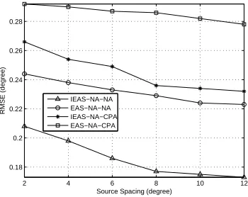
[image:13.612.218.396.309.447.2]al-2 4 6 8 10 12 0.18
0.2 0.22 0.24 0.26 0.28
Source Spacing (degree)
RMSE (degree)
[image:14.612.218.393.132.271.2]IEAS−NA−NA EAS−NA−NA IEAS−NA−CPA EAS−NA−CPA
Figure 5: RMSE results with respect to source spacing.
gorithms, because these algorithms require a set of consecutive co-array lags due to the spatial smoothing operation adopted to deal with the coherent virtual sources arising from the co-array operation. On the other hand, the CS-based algorithm can use both consecutive and nonconsecutive lags of the co-array and therefore are employed here to show the better performance of the IEAS-NA algorithm.
In the CS-based DOA estimation algorithm, the constrained l1 norm minimization problem can be solved using cvx, a package for specifying and solving convex problems [26, 27]. In the formulation, the full angle range from−90◦ to 90◦ is discretized with a step size of 0.05◦. The total number of physical sensors is L = 10, and the parameter settings are according to Tab. 3. The resultant FODLs by EAS-NA-NA isCL¯ =CT¯ = 413, while it is CL = 413, CT = 481 for NA-NA. Both EAS-NA-CPA and IEAS-NA-CPA can generate CL¯ = CL = 273 FODLs, while it is CT¯ = 273 for EAS-NA-CPA andCT = 317 for IEAS-NA-CPA.
In the first simulation, there areK = 2 narrowband source signals with different spacings. The input SNR is 0dB, and the number of snapshots for calculating the fourth-order cumulant matrix is 20000. The DOA estimation result is shown in Fig. 5. Clearly, the root-mean-squared errors (RMSEs) of the IEAS-NA schemes is always lower than that of EAS-NA, due to a greater number of total FODLs and a lager aperture.
Evi-−5 0 5 10 15 20 0.45
0.5 0.55 0.6 0.65
SNR (dB)
RMSE (degree)
[image:15.612.216.395.131.270.2]IEAS−NA−NA EAS−NA−NA IEAS−NA−CPA EAS−NA−CPA
Figure 6: RMSE results with respect to input SNR.
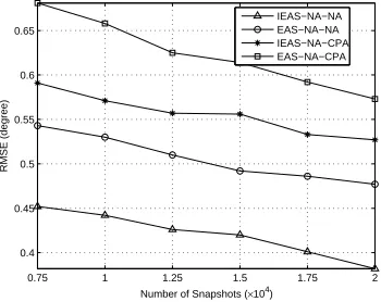
0.75 1 1.25 1.5 1.75 2
0.4 0.45 0.5 0.55 0.6 0.65
Number of Snapshots (×104)
RMSE (degree)
IEAS−NA−NA EAS−NA−NA IEAS−NA−CPA EAS−NA−CPA
Figure 7: RMSE results with respect to the number of snapshots.
dently, the higher the input SNR, the higher its estimation accuracy. The performance of the IEAS-NA schemes is better than that of EAS-NA.
Next, we fix the input SNR to 0dB, and change the number of snapshots. The RMSE results are shown in Fig. 7, where we can see a similar trend and again the IEAS-NA-NA structure has provided the best result for the considered range of snapshot numbers.
[image:15.612.218.393.309.448.2]15 20 25 30 35 500
1000 1500 2000 2500 3000 3500 4000 4500 5000
Number of source signals
[image:16.612.219.395.130.271.2]Minimum number of snapshots
Figure 8: Minimum number of snapshots with respect to source number with a fixed SNR=0dB.
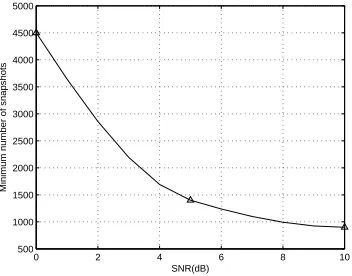
0 2 4 6 8 10
500 1000 1500 2000 2500 3000 3500 4000 4500 5000
SNR(dB)
Minimum number of snapshots
Figure 9: Minimum number of snapshots with respect to source SNR with 33 sources.
other settings are the same as before. As can be seen, at least about 500 to 1000 snapshots are needed to achieve a reasonable result.
6. Conclusion
[image:16.612.218.394.316.454.2]by simulation results, the proposed IEAS-NA scheme has achieved a much better performance than the existing EAS-NA.
7. Acknowledgement
This work was supported by the National Natural Science Foundation of China (61405150 and 61628101).
[1] P. Pal and P. P. Vaidyanathan, “Coprime sampling and the MUSIC al-gorithm,” inProc. IEEE Digital Signal Processing Workshop and IEEE Signal Processing Education Workshop (DSP/SPE), Sedona, AZ, Jan. 2011, pp. 289–294.
[2] C.-L. Liu and P. P. Vaidyanathan, “Remarks on the spatial smoothing step in coarray MUSIC,” vol. 22, no. 9, pp. 1438–1442, Sep. 2015.
[3] P. P. Vaidyanathan and P. Pal, “Sparse sensing with co-prime samplers and arrays,” IEEE Transactions on Signal Processing, vol. 59, no. 2, pp. 573–586, Feb. 2011.
[4] Q. Shen, W. Liu, W. Cui, S. L. Wu, Y. D. Zhang, and M. Amin, “Low-complexity direction-of-arrival estimation based on wideband co-prime arrays,”IEEE Trans. Audio, Speech and Language Processing, vol. 23, pp. 1445–1456, September 2015.
[5] S. Qin, Y. D. Zhang, and M. G. Amin, “Generalized coprime array configurations for direction-of-arrival estimation,” IEEE Transactions on Signal Processing, vol. 63, no. 6, pp. 1377–1390, March 2015.
[6] J. J. Cai, D. Bao, and P. Li, “Doa estimation via sparse recovering from the smoothed covariance vector,” Journal of Systems Engineering and Electronics, vol. 27, no. 3, pp. 555–561, June 2016.
[7] Z. Shi, C. Zhou, Y. Gu, N. Goodman, and F. Qu, “Source estima-tion using coprime array: A sparse reconstrucestima-tion perspective,” IEEE Sensors Journal, vol. 17, no. 3, pp. 755–765, Feb. 2017.
[9] Y. M. Zhang, M. G. Amin, and B. Himed, “Sparsity-based DOA esti-mation using co-prime arrays,” inProc. IEEE International Conference on Acoustics, Speech, and Signal Processing, Vancouver, Canada, May 2013, pp. 3967–3971.
[10] P. Pal and P. P. Vaidyanathan, “Nested arrays: a novel approch to array processing with enhanced degrees of freedom,” IEEE Transactions on Signal Processing, vol. 58, no. 8, pp. 4167–4181, Aug. 2010.
[11] Z. B. Shen, C. X. Dong, Y. Y. Dong, G. Q. Zhao, and L. Huang, “Broadband DOA estimation based on nested arrays,” International Journal of Antennas and Propagation, vol. 2015, 2015.
[12] C. Liu and P. P. Vaidyanathan, “Super nested arrays: linear sparse ar-rays with reduced mutual coupling-part i:fundamentals,” IEEE Trans-actions on Signal Processing, vol. 64, no. 15, pp. 3997–4012, August 2016.
[13] ——, “Super nested arrays: linear sparse arrays with reduced mutual coupling-part ii:high-order extensions,” IEEE Transactions on Signal Processing, vol. 64, no. 16, pp. 4203–4217, August 2016.
[14] J. Liu, Y. Zhang, Y. Lu, S. Ren, and S. Cao, “Augmented nested arrays with enhanced dof and reduced mutual coupling,” IEEE Transactions on Signal Processing, vol. PP, no. 99, pp. 1–1, 2017.
[15] J. F. Cardoso and E. Moulines, “Asymptotic performance analysis of direction-finding algorithms based on fourth-order cumulants,” IEEE Transactions on Signal Processing, vol. 43, no. 1, pp. 214 –224, Jan. 1995.
[16] M. C. Dogan and J. M. Mendel, “Applications of cumulants to array processing.i.aperture extension and array calibration,” IEEE Transac-tions on Signal Processing, vol. 43, no. 5, pp. 1200 –1216, May 1995.
[17] P. Chevalier and A. Ferreol, “On the virtual array concept for the fourth-order direction finding promblem,”IEEE Transactions on Signal Processing, vol. 47, no. 9, pp. 2592 –2595, Sep. 1999.
[19] P. Chevalier, A. Ferreol, and L. Albera, “High-resolution direction find-ing from higher order statistics: The 2q-music algorithm,”IEEE Trans-actions on Signal Processing, vol. 54, no. 8, pp. 2986 –2997, Aug. 2006.
[20] G. Birot, L. Albera, and P. Chevalier, “Sequential high-resolution direc-tion finding from higher order statistics,”IEEE Transactions on Signal Processing, vol. 58, no. 8, pp. 4144–4155, Aug 2010.
[21] P. Pal and P. P. Vaidyanathan, “Multiple level nested array: an effi-cient geometry for 2qth order cumulant based array processing,”IEEE Transactions on Signal Processing, vol. 60, no. 3, pp. 1253–1269, Mar. 2012.
[22] W. K. Ma, T. H. Hsieh, and C. Y. Chi, “DOA estimation of quasi-stationary signals with less sensors than sources and unknown spatial noise covariance: a khatri–rao subspace approach,”IEEE Transactions on Signal Processing, vol. 58, no. 4, pp. 2168–2180, April 2010.
[23] Q. Shen, W. Liu, W. Cui, and S. L. Wu, “Extension of co-prime arrays based on the fourth-order difference co-array concept,” IEEE Signal Processing Letters, vol. 23, no. 5, pp. 615–619, May 2016.
[24] ——, “Extension of nested arrays with the fourth-order difference co-array enhancement,” in The 41st IEEE International Conference on Acoustics, Speech and Signal Processing, Shanghai, China, March 2016, pp. 2991–2995.
[25] J. Cai, W. Liu, R. Zong, and Q. Shen, “An expanding and shift scheme for constructing fourth-order difference co-arrays,” IEEE Signal Pro-cessing Letters, vol. 24, no. 4, pp. 480–484, April 2017.
[26] C. Research, “CVX: Matlab software for disciplined convex program-ming, version 2.0 beta,” http://cvxr.com/cvx, September 2012.