Rochester Institute of Technology
RIT Scholar Works
Theses Thesis/Dissertation Collections
8-1-2010
Single pixel target detection using multispectral
background changes
Alfredo Lugo
Follow this and additional works at:http://scholarworks.rit.edu/theses
This Thesis is brought to you for free and open access by the Thesis/Dissertation Collections at RIT Scholar Works. It has been accepted for inclusion in Theses by an authorized administrator of RIT Scholar Works. For more information, please [email protected].
Recommended Citation
SINGLE PIXEL TARGET DETECTION
USING MULTISPECTRAL BACKGROUND CHANGES
Alfredo Lugo
Submitted in partial fulfillment of the requirements for the degree of M.S. in the Center for Imaging Science,
Rochester Institute of Technology
August 2010
Signature of the Author ________________________________________________
CHESTER F. CARLSON CENTER FOR IMAGING SCIENCE
COLLEGE OF SCIENCE
ROCHESTER INSTITUTE OF TECHNOLOGY ROCHESTER, NEW YORK
CERTIFICATE OF APPROVAL
M.S. DEGREE THESIS
The M.S. Degree Thesis of Alfredo Lugo has been examined and approved by the
thesis committee as satisfactory for the thesis requirement for the Master of Science degree
____________________________________ Dr. David W Messinger, Thesis Advisor
____________________________________ Dr. John R Schott
____________________________________ Dr. Emmett J Ientilucci
THESIS RELEASE PERMISSION
ROCHESTER INSTITUTE OF TECHNOLOGY COLLEGE OF SCIENCE
CHESTER F. CARLSON CENTER FOR IMAGING SCIENCE
SINGLE PIXEL TARGET DETECTION
USING MULTISPECTRAL BACKGROUND CHANGES
I, ALFREDO LUGO, DO HEREBY GRANT PERMISSION TO THE WALLACE
MEMORIAL LIBRARY OF R.I.T. TO REPRODUCE MY THESIS IN WHOLE OR
IN PART. ANY REPRODUCTION WILL NOT BE FOR COMMERCIAL USE OR
PROFIT.
Signature: ___________________________
DISCLAIMER
SINGLE PIXEL TARGET DETECTION
USING MULTISPECTRAL BACKGROUND CHANGES
by Alfredo Lugo
Submitted to the
Chester F. Carlson Center for Imaging Science in partial fulfillment of the requirements
for the Master of Science Degree at the Rochester Institute of Technology
ABSTRACT
Possible methods to help a remote sensing analyst to find a static or moving single
pixel target over vast areas of terrain were examined in this work. Specifically, the
research deals with the particular problem of how to find these targets using multiple
images of the same area that were collected with the same multispectral (6 bands)
imaging sensor but with a background that changes between images.
For this, hyperspectral quadratic covariance-based anomalous change detection
algorithms were investigated to see if they could be used with multispectral data to find a
moving target. In addition, a new method based on change vector analysis was
developed to find a static target. In the case of the moving target problem, the
performance of the Chronochrome, Covariance Equalization, and the Hyperbolic
straight target detection algorithm. In addition, modifications to the covariance-based
algorithms were developed that improved the results. For the static target case, various
multispectral images were “layer stacked” together. Then, the Spectral Matched Filter
hyperspectral target detection algorithm was applied on these data cubes to explore if this
method could help separate a real target from false alarms obtained when simply running
a target detection algorithm on a multispectral data cube.
The analysis demonstrated that a significant reduction in the number of false
alarms can be obtained with these methods when compared to traditional Spectral
Matched Filter (SMF) algorithm to find either static or dynamic single pixel targets of
interest. In addition, the analysis shows the limitations and behavior of these methods
under some of the issues normally encountered in remote sensing imaging. Overall, it
was demonstrated that periodic multispectral imagery collections over a wide area can be
CONTENTS
CHAPTER 1. INTRODUCTION 1
CHAPTER 2. OBJECTIVES 3
CHAPTER 3. BACKGROUND 4
3.1 Static target with hyperspectral sensor 5
3.2 Motion Detection 9
CHAPTER 4. THEORY 10
4.1 Introduction 10
4.2 Quadratic Covariance Based Anomalous Change Detectors 10
4.3 Change Vector Analysis 18
CHAPTER 5. APPROACH 23
5.1 Data Acquisition 23
5.2 Quadratic Covariance Based Anomalous Change Detectors 36
5.3 Change Vector Analysis 42
CHAPTER 6. RESULTS AND DISCUSSION 47
6.1 Covariance-Based Anomalous Change Detection 47
6.1.1 Target changing signature between images 56
6.1.2 Temporal Averaged Baseline 57
6.1.3 Localized Background Statistics 58
6.2.1 Target changing signature between images 63
6.2.2 Degraded Registration 67
6.2.3 Power of Layer Stacking 69
CHAPTER 7. CONCLUSION 71
CHAPTER 8. FUTURE WORK 73
CHAPTER 9. ACKNOWLEDGMENTS 75
LIST OF FIGURES
Figure 1. Pictorial description of the RX algorithm. ...6
Figure 2. Pictorial description of the Spectral Matched Filter… ...8
Figure 3. Target moving spatially as a function of time. ...9
Figure 4. Performance comparison for anomalous change detectors ...17
Figure 5. Change vector on 2-band space. ...19
Figure 6. Seattle Washington land changes. ...20
Figure 7. Signatures of two similar targets after layer stacking. ...22
Figure 8. Space Shuttle from space as it is transported to launch pad. ...25
Figure 9. Close up of Space Shuttle as it is transported to launch pad. ...25
Figure 10. Landsat image of Cape Canaveral coast in Florida. ...26
Figure 11. Space Shuttle circled on band 5 of baseline image. ...27
Figure 12. Cape Canaveral reconciled images. ...28
Figure 13. Alabama images. ...29
Figure 14. Hydice images used. ...32
Figure 15. Hydice images close ups with targets used. ...32
Figure 16. Close up of baseline image bottom left runway. ...34
Figure 17. Space Shuttle added to Alabama image. ...36
Figure 18. Space Shuttle movement in Cape Canaveral. ...37
Figure 19. Cape Canaveral target locations. ...37
Figure 20. Alabama target locations. ...38
Figure 21. Steps for the covariance based algorithms target detection study. ...39
Figure 22. Possible target changes. ...40
Figure 23. Temporal Moving Average Description. ...41
Figure 24. Steps for the layer stacking target detection study. ...44
Figure 25. One pixel misregistration for layer stacking. ...45
Figure 26. 3 layer stacked representation. ...46
Figure 28. Clouds in May 09 image (image #5). ...50
Figure 29. Results for the Cape Canaveral target algorithms comparison. ...51
Figure 30. Algorithm comparison for the Cape Canaveral Jan 07 image. ...53
Figure 31. False Alarm Rate (%) average versus PSNR for the various target locations...55
Figure 32. Alabama July 2009 image anomalies. ...56
Figure 33. Results comparison between the changed target and the not changed target. ...57
Figure 34. Temporal 2-image averaged baseline results versus a one image baseline. ...58
Figure 35. Change Vector Analysis results for the Cape Canaveral images. ...62
Figure 36. Change Vector Analysis results for the Alabama images. ...62
Figure 37. Results comparison between the 10% “blended” static target and the no changed target. ...64
Figure 38. Zoom of baseline image showing the exact location of target by road ...65
Figure 39. Google Earth image of target pixel area. ...65
Figure 40. Picture of road junction shows target pixel area. ...66
Figure 41. Results comparison between the 10% and 50% “blended” static target. ...67
Figure 42. Misregistration effects on SMF results of stacked images ...68
Figure 43. SMF false alarms comparison between multiple number of stacked images. ...69
LIST OF TABLES
Table 1. Coefficients for the Quadratic Covariance Anomalous Change Detectors. ...16
Table 2. Landsat 5 TM spectral bands ...24
Table 3. PIF (Runway) Statistics for Cape Canaveral first image pair. ...35
Table 4. Algorithms comparison for the Cape Canaveral target by the road....48
Table 5. Algorithms comparison for the Cape Canaveral target by launch pad. ...51
Table 6. Algorithms comparison for the Alabama target by road bend....54
Table 7. Algorithms comparison for the Alabama target by middle of the fields. ...54
Table 8. Global vs local error comparison for the Cape Canaveral images. ...59
Table 9. Global vs local error comparison for the Cape Canaveral images. ...59
Table 10. Global vs local error comparison for the Alabama images. ...59
Table 11. Global vs local error comparison for the Alabama images. ...59
Table 12. Global vs local error comparison for the Hydice images. ...60
Chapter 1.
Introduction
One of the main uses of remotely acquired imagery is to try to find small objects of
interest over vast areas of terrain. These objects are commonly known in the remote sensing
community as anomalies (if we are just looking for what is different from the rest of the scene)
or targets (if we are interested in a specific known object or family of related objects). To find
these objects, the analyst would normally collect a hyperspectral image cube from the scene of
interest and then apply one of the many algorithms available to tackle this kind of problem. As
explained by Schott (2007), the analyst would probably try first to find the objects using
deterministic, statistical, or spectral feature algorithms by solely using the data contained in the
image. Then, if better results are needed, he will add physics based models to the analysis.
A problem arises if instead of hyperspectral data we only have data from a multispectral
sensor like WorldView, GeoEye, Landsat, etc. In this case, especially for single pixels or
sub-pixel targets, the anomaly/target finder algorithms that rely on hyperspectral data would yield too
many false alarms. This, of course, is not desired and could make the task of finding these
anomalies/targets impossible if time is of the essence and access to the scene is limited or not
available (like for most military applications).
To improve the chances of finding the targets/anomalies, other methods have been
developed that make use of the ability of a sensor to revisit the same scene at different times. If
the revisit time is short enough and the background does not change, simple change detection or
track-before-detect algorithms could be used to find single pixel level changes or moving targets.
Nevertheless, if the revisit time is longer (weeks, months, or years) or something affects greatly
the overall scene in a short period of time (e.g. rain), the background changes (in illumination,
detection and track-before-detect methods useless. This lead to the problem studied here : how
to find a static or moving single pixel target using multiple images of the same area that were
collected with the same multispectral (6 bands) imaging sensor but with a background that
changes between images.
To solve this problem, quadratic covariance-based anomalous change detection
algorithms were investigated to see if they could be used with multispectral data to find a moving
target and if change vector analysis could be used somehow to find a static target. In the case of
the moving target problem, the performance of the Chronochrome (Schaum & Stocker, 1997),
the Covariance Equalization (Schaum & Stocker, 2003), and the Hyperbolic (Theiler, 2008)
anomalous change detection algorithms were compared relative to each other and to a standard
target detection algorithm. In addition, modifications to the covariance-based algorithms were
developed to improve their results. For the static target case, various multispectral images were
“layer stacked” together and then hyperspectral target detection algorithms were used on these
data cubes to explore if this method could help separate a real target from false alarms obtained
when just running a target detection algorithm on a multispectral data cube.
This thesis is a summary of the work accomplished to help answer the stated problem. It
is presented in the traditional thesis report format. In chapter two, the objectives of the research
are stated. In chapter three, a background about the specific problem under consideration is
presented as well as traditional target detection algorithms. In chapter four, quadratic
covariance-based anomalous change detector algorithms and change vector analysis theory is
covered. In chapter five the specific approach used is described. In chapter six, the results are
presented and discussed. Lastly, chapters seven and eight give conclusions and ideas for
Chapter 2.
Objectives
The specific objectives of this research were:
1. Understand the physics of reflectivity, absorption, and radiative transfer as they pertain to the
problem.
2. Understand how to use the Geo data provided with Landsat images to register images
together.
3. Study how pre-processing steps (collection noise, registration, etc) affect algorithm
performance.
4. Study how to predict target signature change from one image to another, and how much the
errors in this prediction contribute to the final target detection error.
5. Find out how the covariance-based anomalous change detection algorithms perform with this
kind of spectral-temporal data.
6. Investigate how the performance of the covariance based anomalous change detection
algorithms change when using a temporal average for baseline image.
7. Investigate how the performance of the covariance based anomalous change detection
algorithms change when using local background mean errors instead of global background
mean errors.
8. Develop a way to use change vector analysis to improve upon the results obtained by
Chapter 3.
Background
As stated in the introduction, the problem this project addresses is how to find a small
(single pixel) target over a vast area of interest using a multispectral sensor when all we have
available are images that, although of the same physical area, have different looking
backgrounds. As explained, this normally happens most when there is a big overall change in
the scene in a short period of time (like fire or rain) or when the images are taken months or
years apart from each other. For example, this can be the case of a military application where we
are trying to quickly find a small mobile target of interest but all we have over the area is a
multispectral sensor, which last collected on the area months ago. Another real case scenario
would be a static (either permanent or temporary) target of interest which is very difficult to find
in a single image because of its size and spectral signature compared to its background (like a
camouflaged bunker or a missile launcher). The significant background changes between data
collections, the low spectral resolution (6 bands from visible wavelengths to short IR) of the
sensor, and the spatial aspects of the targets (single pixel and dim) greatly restrict the type of
algorithms we could use to find these targets.
There are many proven ways to solve similar problems but unfortunately, although very
helpful for some applications, they fall short under these restrictions. Nevertheless, the methods
explored for this thesis have embedded some of these traditional algorithms. Therefore, a
3.1 Static target with hyperspectral sensor
On the more static and higher spectral resolution data end of the spectrum you have the
traditional problem of finding a target or anomaly using a hyperspectral data cube. To
accomplish this, we have numerous deterministic, statistical, or spectral feature methods at our
disposal. Two of the best known statistical methods are the RX and the Spectral Matched Filter
(SMF)algorithms. Developed by Reed & Yu (1990), the RX algorithm is designed for the case
where we do not have or are not interested in the target signature but instead we are trying to find
pixels that are spectrally different from the background. Mathematically, the RX algorithm can
be expressed as
= − − , (1)
where m is the mean and S the spectral covariance matrix of either the whole image or a local
area around the pixel in question (x). As can be noticed, the algorithm provides the squared
Mahalanobis or statistical distance from each pixel to the mean (global or local). Then, this
distance is compared against an established threshold that separates the background from the
anomalous pixels. Any pixel far away from the mean will be considered an anomaly and any
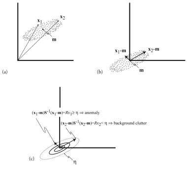
pixel within the threshold distance will be considered as part of the background. Figure 1,
Figure 1. Pictorial description of the RX algorithm.
As stated by Schott (2007), Figure 1a is a simplified 2-D plot of the data space
highlighting two pixels and Figure 1b graphically demonstrates the aftermath after subtracting
the mean (m) from the data (x). Finally, Figure 1c graphically demonstrates the isoprobability
contours associated with the normalization by the covariance showing that in statistical distance,
On the other hand, if the target spectral signature is known, we can use the Spectral
Matched Filter. Mathematically, this filter can be expressed similar to the RX algorithm as
= − − , (2)
where t is the target spectral signature. As explained by Schott (2007), the difference between
the RX algorithm and the SMF algorithm is that instead of calculating the square statistical
distance from each pixel to the background mean, when using SMF we are first transforming the
demeaned target vector and image data into a space that is normalized by the square root of the
background covariance matrix. Then, we project the whitened image vector onto the whitened
target vector. This two-step process can be understood easier if we rewrite equation (2) as
= − − . (3)
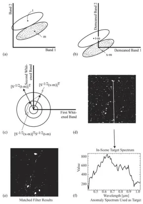
Figure 2, from Schott (2007), illustrates the two-step process in parts a, b, and c. In part
e, we can see the result of using the signature (part f) of one of the anomalous pixels found using
Figure 2. Pictorial description of the Spectral Matched Filter. (a) (b) (c) Conceptual representation of the two-step
process in equation 3. (d) (e) (f) The signature (f) of one of the anomaly pixels found using the RX algorithm (d)
can be used to decrease the number of false alarms using the SMF algorithm (compared with e ).
More details of these and many other deterministic, statistical, spectral feature methods
and even some physics based methods that spawned from these basic algorithms can be found in
Schott (2007). Nevertheless, the problem with our case is that we normally do not have enough
information on a multispectral data cube to separate a small dim target from background using
3.2 Motion Detection
There is also the case of a target moving within a sensor field of view over a short
amount of time but which shows up on consecutive images. A representation of the problem can
be seen in Figure 3; as obtained from Bruton & Bartley (1986). As can be noticed in the Figure,
the spatial movement of the object will be seen in the spatial-temporal domain as a set of points
through the frames connected by lines that have heading in accordance to the object’s movement.
Figure 3. Target moving spatially as a function of time.
In this case, for very dim and small targets there are numerous track-before-detect
algorithms available that could be used to find a moving target. Nevertheless, for our specific
problem, these methods do not work as the time between frames will be too great or the
background changes too drastic for these algorithms.
Another traditional way used to find a target that moved between images is simply to
subtract one image from another and then call targets those pixels with the greatest difference.
Although this method can give you pretty good results for simple changes between images, it
breaks down for multispectral images with completely different background changes and
Chapter 4.
Theory
4.1 Introduction
Now that we understand the problem, let us look at the theory behind the specific
algorithms explored for this thesis. Even though there is some overlap between them, basically
they can be divided into two categories; the ones that are primarily used to find a moving target
(quadratic covariance based) and the one (change vector analysis) developed here to find a static
target.
4.2 Quadratic Covariance Based Anomalous Change Detectors
As named by Theiler (2008), these algorithms encompass all those created to find
anomalous changes between two spectral images of the same area by using the covariance
properties of the data and that “can be expressed as quadratic functions of the input data”. They
were created to overcome the challenge of how to find an anomalous change without triggering
too many false alarms due to what Schaum & Stocker (1997) call “clutter evolution”; referring to
how each class of material that makes up the background clutter for an image changes in a
uniform way from one image to the other. As a simplistic example, these algorithms will not
flag grass that changed color from green in fall to brown in winter as an anomalous change
(unless there is only a small patch of grass in the whole image).
Mathematically, similar to the RX and SMF algorithms already discussed, these
algorithms provide a score on how anomalous the change was for a pixel from one image to
another. In general, they accomplish this by comparing how much each individual pixel changed
To accomplish this, all of them start by mean-centering the values of the pixels in the two
images to be compared. In this way, the expected value of the pixels on the first image and the
expected value of the pixels from the second image both equal zero. Using the same convention
as that found in most of the related literature, for the remainder of this proposal the
mean-centered value of a pixel from the first image will be called x and the mean mean-centered value from
the same pixel on the second image will be called y. With these mean-centered spectral data
cubes, the next step is to calculate the spectral covariance for each image; X=Cov(x,x) and
Y=Cov(y,y). Then, some of the algorithms require a cross covariance between images defined
as
C = Cov(y,x) = E [(x-E[x])·(y-E[y])] = E[x·y] – E[x]·E[y], (4)
where E[x] is the expected pixel value for the first image and E[y] the expected pixel value for
the second image.
To make this cross covariance work, the images should be registered accurately down to
the single pixel level. Because registration techniques are so numerous and varied they will not
be detailed in this report. Instead, only the specific way in which some of the test images were
registered will be discussed (in the methodology section). For details on general registration
techniques, see Wolf & Dewitt (2000) and Gonzalez & Woods (2008).
4.2.1 Chronochrome Algorithm
The Chronochrome algorithm is the oldest of the change detector algorithms considered
here. As explained in detail by Schaum & Stocker (1997) and Schaum & Stocker (2003), it
between images (C) to create a linear estimate of the second image from the first image. That is,
using the x and y convention for the first and second image respectively
≈ (5)
where L is the linear estimator matrix. From here, Schaum & Stocker (2003) derive the error
[ε
=
y – Lx
)] between the real second image and the linear estimate of the second image byfinding a solution for the linear estimator in L= CX-1 and therefore proving that the error (ε)
between the estimated and real second image equal
= − . (6)
This error matrix will of course have the same spectral channels as the compared images.
Therefore, once this matrix has been computed, the anomalous changes between the two images
are found by using an anomalous change detection algorithm (like the RX algorithm) on the error
matrix using the error matrix global statistical information. As previously discussed already in
section 3.1, any pixel with a large score from the RX algorithm is a pixel with a change between
images that is too far from the norm when compared to the changes exhibited by other pixels
with approximately the same spectral signature on the first image.
4.2.2 Covariance Equalization Algorithm
This algorithm was created to address one of the fundamental problems with the
Chronochrome algorithm; its necessity to have pixel level registration accuracy between images.
Similar to the Chronochrome algorithm, the Covariance Equalization algorithm first estimates
computes the error between the predicted values and the real values. Schaum & Stocker (2003)
derive the linear estimator matrix for general imaging problems to be
! = " # #. (7)
In this case, the subscript CE has been added to the linear estimator L to differentiate it from the Chronochrome (CC) linear estimator. The R is an orthonormal matrix which varies according to the imaging application (3-D Imaging vs Hyperspectral Imaging). In the case of hyperspectral
imaging, Schaum & Stocker (2003) have found that making R the identity matrix works well. Therefore, the Covariance Equalization error equation for hyperspectral remote sensing imaging
can be expressed as
= − " # #. (8)
To make R equal the identity matrix applies as long as there are no physical changes in the environment between the images that would increase variability in some wavelengths while
decreasing it in others. As they explain, normal remote sensing changes like changes in apparent
path radiance, illumination levels, scattering from varying concentrations of aerosols, and in
sensor electronic gains are all either explained in the first order statistics from the data or will
affect all wavelengths in a correlated fashion. Both of these cases will not affect the math behind
equation (6). Therefore, because multispectral and hyperspectral remote sensing imaging are
4.2.3 Hyperbolic anomalous change detection
As described by Theiler (2008), both the Chronochrome and the Covariance Equalization
algorithms use the error between the second image and the transformed (by the linear estimator
matrix) first image to find anomalous changes between images. On the other hand, the
Hyperbolic change detection algorithm fuses together both images and treats them as one large
image. Theiler (2008) derives the final Hyperbolic anomalous change detection formula. He
starts by defining how the probability distributions for the x and y values on each pixel can be
used to find an anomalous pixel and then uses the assumption that the data distribution is
Gaussian to describe the probability functions in terms of the covariance and cross-covariance
matrices. In this way, he finally obtains the anomalousness equation
$, = % &'()*+,-
., (9)
where
'()*+, = - " .
− - 00 ".. (10)
In contrast to the RX algorithm used as part of the Chronochrome and Covariance
Equalization algorithms, the anomalousness score when using equation (9) can be positive or
negative. Therefore, the absolute value of the anomalousness score should be taken before
deciding how anomalous a pixel is compared to the others. One final detail to consider for this
algorithm is that, as stated by Theiler (2008), even though this quadratic expression was
developed assuming Gaussian distributed data, it can be applied regardless of the actual
distribution. For comparison purposes, it is important to mention that the SMF algorithm relies
performs well for other distributions. Therefore, when comparing the SMF versus covariance
based algorithms, any background deviations from a perfect Gaussian distribution will probably
affect all algorithms compared the same way.
Even though the three algorithms presented are the main Quadratic Covariance Based
Anomalous Change Detectors, they are not the only ones available. Variants of them are the
Optimal or Diagonalized Covariance Equalization (Theiler, 2008) and the Subpixel Hyperbolic
(Theiler, 2008). In addition, there are others that although not that powerful, are comparatively
simpler and could also be very useful depending on the application. These are the Simple
Difference and the RX on a fused image. Theiler (2008), transforms all the known equations for
all of the Covariance Equalization algorithms into a common function
$, = % &' -., (11)
where the coefficient matrix Q is different for each algorithm. If we want (or need) to use
whitened data where
0 = #, (12)
1 = " #, (13)
and
2 = " # #, (14)
we can still obtain an anomaly score with these algorithms by using
Table 1 of Theiler (2008)
whitened data and therefore is included
difference between the various algorithms
Table 1. Coefficients for the Quadratic Covariance Anomalous Change Detectors
4.2.4 Quadratic Covariance Based Anomalous Change Detector Results
In addition to Schaum &
the Chronochrome and Covariance Equalization algorithms,
comparison test between all the algorithms from
channel AVIRIS image taken of a coastal area in Florida. He manipulated the image to induce
pervasive changes (smoothing, noise, spectral splitting, and misregistration)
and induce anomalous changes in a handfu
the original/changed image pair to study how the algorithm performance varied with
background pervasive changes. He induced
(2008) summarizes all the coefficient matrices in either normal or
and therefore is included below so the reader can have a better idea of
between the various algorithms.
for the Quadratic Covariance Anomalous Change Detectors.
4.2.4 Quadratic Covariance Based Anomalous Change Detector Results
Stocker performing individual tests with hyperspectral data on
the Chronochrome and Covariance Equalization algorithms, Theiler (2008) performed a
comparison test between all the algorithms from Table 1. His study was based on a 224 spectral
channel AVIRIS image taken of a coastal area in Florida. He manipulated the image to induce
(smoothing, noise, spectral splitting, and misregistration) on the whole image
anomalous changes in a handful of pixels. Then, he applied the algorithms against
the original/changed image pair to study how the algorithm performance varied with
He induced the four different pervasive changes on
in either normal or
have a better idea of the
4.2.4 Quadratic Covariance Based Anomalous Change Detector Results
performing individual tests with hyperspectral data on
performed a
s based on a 224 spectral
channel AVIRIS image taken of a coastal area in Florida. He manipulated the image to induce
the whole image
applied the algorithms against
the original/changed image pair to study how the algorithm performance varied with the different
create four different background changed images to which he then added anomalous changes.
He generated the anomalous pixels by either removing pixels and changing them with pixels
from different parts of the image or by darkening and brightening the pixels. Finally, he
analyzed how well the algorithms performed by creating Receiver Operating Characteristic
(ROC) curves from the data using the prior knowledge of the total number of anomalous pixels.
A figure that shows the algorithms’ ROC curves under the four pervasive background changes
for full pixel anomalies taken from the same image is shown in Figure 4. The ROC curves
correspond to the following background changes: (a) smoothing, (b) noise, (c) spectral splitting,
and (d) single pixel misregistration.
Figure 4. Performance comparison for anomalous change detectors with pervasive background changes
Overall, it can be noticed in Figure 4 that misregistration and smoothing are the pervasive
changes that affect the algorithms the most. This was also seen on most of the other ROC
figures in the paper. Problems with misregistered images are expected as the algorithms are
designed to compare a pixel on the first image versus specifically the same pixel on the second
image and some even use the images’ cross covariances or fuse the two images together.
Smoothing affects the results more than noise and spectral-splitting as smoothing changes every
pixel by different localized values which cannot be explained by the image global statistics;
changing the image in a way that is not reflected in the image covariance.
By comparing the different ROC curves within the graphs, we can see that the Subpixel
Hyperbolic algorithm performed the best followed by the more basic Hyperbolic algorithm. This
was also the case on the other figures presented in the paper. Therefore, according to the paper,
the Hyperbolic algorithm is the best when compared to the other algorithms with the exception
of its own variant, the Subpixel Hyperbolic algorithm. This result was corroborated as part of
the thesis.
4.3 Change Vector Analysis
As stated already, in addition of trying to find moving targets by using the
covariance-based algorithms, work was performed to try to find very dim single pixel targets that did not
move from one image to the other using the advantage of having multiple collections over the
scene. As previously stated, the background science behind the idea used stems from something
called Change Vector Analysis.
Change vector analysis refers to the idea in which the location of a pixel from one image
in the same spectral space. The distance and direction the pixel “moves” in this n-band spectral
space creates the change vector. Pixels that change significantly between images will have
significant change vectors while pixels that do not change too much will have small vectors.
Figure 5, obtained from Johnson & Kasischke (1998), explains this graphically.
Figure 5. Change vector on 2-band space.
The literature on change vector analysis uses the idea to detect and classify changes over
large areas of images for purposes like land classification, crop/forest changes, etc. For example,
Johnson & Kasischke (1998) used the changes between a Landsat TM image of Seattle
Washington taken in July 1984 and one taken August 1992 to find new urban development that
occurred over the area between that timeframe. They accomplished this by first performing a
full dimensional change vector analysis on the image pair to find all the changes and then
selecting from these areas that which actually changed from vegetation to urban material. This
was carried out by using the Maximum Likelihood Classification method (see Schott, 2007) on
each image and then comparing the results against one another for the areas already flagged by
analysis resulting change image in which color is used to represent all areas with changes. On
the other hand, the red color on the right image is used only to point out vegetation to developed
land changes and was created after combining the results on the left image with the results of the
Maximum Likelihood Classification algorithm.
Figure 6. Seattle Washington land changes: left = all changes; right = vegetation to urban.
After an extensive literature search, nothing was found about how to use change vector
analysis to find single pixel or sub pixel targets of interest. Therefore a different approach is
needed that could mix the proven ways to find targets using target detection algorithms with the
power that change vector analysis can provide with multiple images of an area over long time
intervals or global background uniform changes. The new approach is simple: we create a false
hyperspectral image out of our multiple multispectral images and then use a hyperspectral target
detection algorithm to find which pixel(s) belong to change vectors that are most similar to a
change vector that a particular target of interest would have. In other words, we will create a
target change vector signature and then look for the pixel with the most similar change vector.
However, to be able to create this false hyperspectral image, we first need to
radiometrically normalize the multispectral input images. This is necessary since the same target
vary the signature that a target of interest would have from one image to the next and leaving the
images the same. Since both methods should work the same, only the first (image to image
normalization) method was used for this thesis.
To accomplish this, there are various techniques that have been developed. One of the
most commonly used is that described by Schott, Salvaggio & Volchok (1988) which consists of
using materials in the scene whose reflectance distribution is believed to be constant between
images to correct for environmental (atmospheric, illumination) and sensor response differences
that occurred between collects. These materials are called Pseudo-Invariant Features (PIF) and
are simply manmade surfaces like roads, runways, etc.
If we want to use this method to normalize two images, we start by selecting
corresponding pixels from the materials mentioned already. Then, we calculate the mean and the
standard deviation for each group of pixels to use them to obtain the slope (m) and intercept (b)
of a linear equation that relates image 1 to image 2 as in
4 = 4+ 6, (16)
where DC1 represents the digital count of a pixel in image 1 and DC2 represents the digital count
of the same pixel in image 2. We can express the slope and intercept as
=77
(17)
6 = 489:− 489:, (18)
where DC1avg and σ1 correspond to the mean and standard deviation for the group of pixels on
group of pixels on image 2. Once the multispectral images we want to use are radiometrically
normalized, we create the false hyperspectral image by layer stacking the various images. The
idea is that pixels with similar signatures on one multispectral image will be spectrally different
on other subsequent images. In this way, false alarms will be reduced when using target
detection algorithms. Figure 7 attempts to graphically explain the idea. In this Figure, the x axis
represents how the bands of a 6-band multispectral sensor would be spectrally “layer stacked” to
form the false hyperspectral image. As can be noticed in the figure, the two targets (one with red
signature and one with blue) have the same signature (superimposed showing as blue) on most of
the 6-band sets but differ on two of these sets. That difference could be used by a hyperspectral
target detection algorithm to identify which one is the target of interest and which one is not.
Chapter 5.
Approach
5.1 Data Acquisition
The first step on any target detection research project is to collect data. For this thesis,
the primary sensor used was the Thematic Mapper (TM) sensor on Landsat 5; one of NASA’s
Earth-observing satellites. This sensor, a copy of the Landsat 4 TM sensor, has been collecting
Multispectral images since 1984. These images are all available for free at
http://glovis.usgs.gov/ImgViewer/Java2ImgViewer.html. From there, multiple images of the
same area that were collected months or years apart from each other can be downloaded. Out of
the 7 spectral bands per image (see Table 2 for details) only the reflective bands (1-5 and 7) were
used due to the radiometric phenomenology collection differences between the reflective and
emissive parts of the light spectrum (see Schott 2007). The other reason the Thermal band (# 6)
was not used was to avoid any registration issues that could have surfaced as a result of the
sensor pixels projecting a ground sample distance (GSD) of 120m for that band versus only 30m
for all the other bands. For more details on the Landsat 4 and 5 program and the specifics of the
Table 2. Landsat 5 TM spectral bands
Band Number Portion of Spectrum Wavelength Interval (µm)
Ground Sample Distance (m)
1 Visible 0.45 – 0.52 30
2 Visible 0.52 – 0.60 30
3 Visible 0.63 – 0.69 30
4 Near-Infrared 0.76 – 0.90 30 5 Near-Infrared 1.55 – 1.75 30
6 Thermal 10.40 – 12.50 120
7 Mid-Infrared 2.08 – 2.35 30
To use a real target signature and because of the low spatial resolution (30m GSD) of the
Thematic Mapper collections, the Space Shuttle was the target used for all the Landsat images.
Specifically, the signature obtained when the Space Shuttle was on top of its carrier was used.
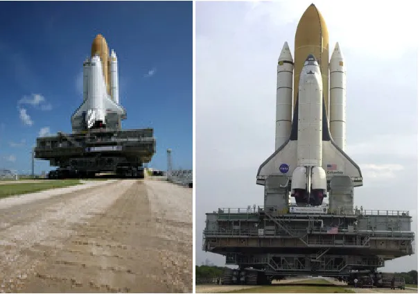
Figure 8 is NASA’s photograph ISS010-E-23035 obtained from Google Earth where we can see the Shuttle as it is transported from the vehicle assembly building to the launch pad assembly
area at the Kennedy Space Center in Florida. From it we can get a good feeling for the relative
size and reflectivity of the Space Shuttle and carrier compared to their background at the
Figure 8. Space Shuttle from space as it is transported to launch pad.
On March 4th 2007, the Space Shuttle for mission STS-117 was transported back from the
launch pad to the vehicle assembly building due to damage suffered during a hail storm the week
before. Fortunately, Landsat 5 collected an image of this event. This image, collected at 11:43
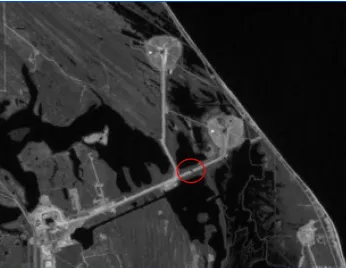
a.m. Eastern Time on that day, is presented in Figure 10 below (copied from the preview screen
of the US Geological Survey (USGS) Global Visualization Viewer website).
Figure 10. Landsat image of Cape Canaveral coast in Florida.
After downloading the image file from the USGS website, decompressing the image, and
stacking the bands using ENVI to create the multispectral image, a small area around the
Kennedy Space Center was cut to obtain the image to be used as the Cape Canaveral baseline
image. Figure 11 displays band 5 (1.55-1.75 µm) data from this baseline image. As annotated
Figure 11. Space Shuttle circled on band 5 of baseline image.
Once we have the baseline image (Figure 11), we can obtain other images of the same
area by first downloading big images (Figure 11 size) of the general area and then using ENVI to
cut out of them approximately the same area as the baseline image. Since the images
downloaded from the USGS website contain geolocation metadata that is read by ENVI, the
other images were cut in ENVI by first selecting the baseline image as a Region of Interest (ROI)
in the big image and then reconciling via map this ROI to the other big images. The six images
that were used in addition to the baseline image for the Cape Canaveral area were processed in
this way and are included in Figure 12. Each Cape Canaveral image used is 369 by 360 pixels in
Figure 12. Cape Canaveral reconciled images. Top left = Jan 07,, Top Center = May 07, Top Right = Jan 09
Bottom Left = Mar 09, Bottom Center = May 09, Bottom Right = Feb 06.
In addition to the Cape Canaveral set of images, a set of Landsat images each one 402 by
398 pixels in size (total of 159996 pixels) from about 40 miles west of Montgomery Alabama
was used as part of this research. A baseline image was selected and five other images were
reconciled against the baseline image using the same procedure mentioned above. The Alabama
baseline image as well as the five Alabama reconciled images are presented in Figure 13. For
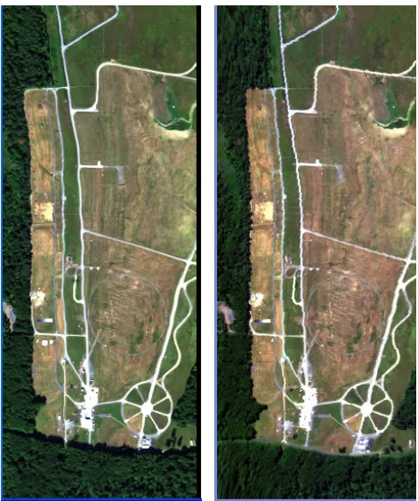
Figure 13. Alabama images. Top left = Jan 10,, Top Center = Mar 08, Top Right = Jul 09
Bottom Left = Nov 04, Bottom Center = Dec 04, Bottom Right = May 08.
All the Alabama images downloaded from the USGS website and cut with ENVI were
almost perfectly registered against one another thanks to the original images downloaded being
processed to Standard Terrain Correction (Level 1T). As explained in the website
https://landsat.usgs.gov/Landsat_Processing_Details.php, this level of processing “provides
systematic radiometric and geometric accuracy by incorporating ground control points while
employing a Digital Elevation Model (DEM) for topographic accuracy”. Therefore, when ENVI
cut the areas shown in Figure 13 out of the big (Figure 10 size) original Landsat images, the
registered set of images in Figure 13. The amount of error in this registration was manually
corroborated to be sub pixel for each Alabama image pair used. Therefore, no further
registration was applied.
On the other hand, the Cape Canaveral images shown in Figure 12 were not that well
registered against one another. The reason was that the big images where they came from were
not processed to Level 1T correction but only to Level 1G correction (Systematic Correction).
According to the USGS website, this level of correction does not use Digital Elevation Models
but only use data collected by the sensor and spacecraft, making the registration error around six
pixels (1 sigma) for low-relief areas at sea level. The reason why some images are processed at
this level versus the better 1T level is that for some images, there are not good ground control
points or necessary elevation data. As can be noticed in Figure 10, the big images used to get
Figure 12 images fall into this category of lack of necessary ground control points due to all the
water in the images.
To test the algorithms it is necessary to start with pixel to pixel registration accuracy.
Therefore, the registration errors obtained using ENVI for the Cape Canaveral images had to be
eliminated. This means that the Cape Canaveral images in Figure 12 had to be manually
registered by the traditional method of selecting ground control points and matching them to
each other in pixel coordinates. Fortunately, Landsat is in a Polar Sun-Synchronous orbit which
revisits the same spot every 16 days. Therefore, the images were taken from the same angle
making a simple translation the only correction needed.
Although most of the images used for this thesis were obtained by the Landsat TM
sensor, two images from the Hyperspectral Digital Imagery Collection Experiment (Hydice)
0.4 µm to 2.5 µm range of the light spectrum and is operated out of an airborne platform in
pushbroom mode.
The two images were part of an experiment by the Hydice Program Office in 1995 in
support of the Forest Radiance experiment conducted as part of the Hyperspectral Support to
Military Operations program. The images were collected over the Aberdeen Proving Grounds 20
miles northeast of Baltimore and were taken at a good enough altitude to have pixel GSD of 3
meters; perfect to obtain single pixel targets. The collects were staged to have the targets
completely visible by the left tree line on the first image and not visible on the second image.
Close ups of the target line for both images are shown in Figure 15; which were taken at a lower
altitude than the ones used in Figure 14. Bergman (1996) provides more specifics on these
collects.
Out of the 210 possible spectral bands, only 145 were usable due to atmospheric
absorption or sensor artifacts. Then, these were spectrally re-sampled to match the 6 Landsat
bands used for this research (see Table 2). Also, 5 columns and 10 rows of each image were cut
because of registration and computing time issues to end up with a 470 by 214 image for a total
of 100580 pixels. Nevertheless, different to the Cape Canaveral and Alabama image sets, no
targets were synthetically added or the images radiometrically corrected in any way. Instead, the
targets used were the same ones already there. Out of all the targets available in Figure 14 (the
image used) that are perfectly visible in Figure 15, only 4 were used for the analysis to make sure
that the pixels used were completely filled by a target. The targets used have been identified in
Figure 14. Hydice images used. Left = Image with targets, Right = Image without targets
Target #1
Target #2
Target #3
[image:45.612.82.439.382.692.2]Unfortunately, out of the times the shuttle/transporter combined target was moving from
the assembly building to the launch pads, it was found on the Landsat database only once (Figure
10). Therefore, the shuttle/transporter target from the baseline image had to be synthetically
added into the other Cape Canaveral images. To achieve this, there were many approaches that
could have been used depending on the level of accuracy needed. For the purposes of this thesis,
a simple copy and paste of the target from the baseline image to the other Cape Canaveral
images would not have been appropriate because in real life the target signature would have
changed in accordance to illumination conditions, atmospherics, etc. Therefore, some sort of
radiometric correction of the target or images was needed to “move” the target from the baseline
image to the other images. To avoid the associated errors of a full blown radiometric
normalization between images and because in real life a target’s overall reflectance can change
during months or years timeframe spans (due to paint chipping, dirt vs clean, different cargo on
top, etc), the radiometric correction was limited to the average radiometric difference between
images.
This was accomplished by using Pseudo Invariant Features (PIF) in a close but different
manner as the method presented in section 4.3. Because the correction wanted was only for the
average difference between images, the standard deviation relation of equation (17) was not used
but instead a slope (m) of unity in equations (16) and (18) was used. The PIF used for the Cape
Canaveral images was the center of the runway on the bottom left of the images (close up on
Figure 16); from which 27 really good pixels were extracted. The means and standard deviations
of these pixels for the first two Cape Canaveral images compared (baseline vs Jan 07) are
presented in Table 3. It is important to mention at this point that the associated signature errors
or to correct an image against a baseline image are not important for this thesis. The reason is
that this work is limited to comparisons between specific algorithms for targets and image
combination examples that were set up in such a way that any signature error would affect both
sides of the comparisons generally in the same way. This thesis does not try to answer absolutes
about the number of false alarms expected in general with these algorithms. In real life, the
results would be dependent on the specific combination of targets, backgrounds,
[image:47.612.196.417.281.500.2]pseudo-invariant features, and prior knowledge of the target signature.
Table 3. PIF (Runway) Statistics for Cape Canaveral first image pair.
Landsat Band # Mean Baseline Mean Jan 07 Std Baseline Std Jan 07
1 131 112 3.5 5.7
2 67 57 2.6 3.5
3 78 67 3.4 4.7
4 82 69 2.7 3.9
5 160 143 2.3 4.2
7 85 77 1.1 1.9
As stated already, in addition to the Cape Canaveral images, a set of images of an area 40
miles west of Montgomery Alabama was used both to find moving targets as well as static
targets. However, there were no real targets in the area that could be used for this research.
Consequently, the Space Shuttle was synthetically added to all Alabama images. In theory, any
kind of fictitious target with any kind of fictitious spectral signature could have done the job but
to try to keep at least something in common between the Cape Canaveral images and the
Alabama images, the Space Shuttle was chosen as the target.
To “move” the Shuttle from Cape Canaveral to Alabama, the signature of the Shuttle was
pulled out of the Cape Canaveral baseline image and then this signature was corrected for the
band by band spectral difference between this image and an Alabama image taken by Landsat
January 10, 2010. This was accomplished to try to make the target have the same contrast
against the Alabama image background as it did on its original Cape Canaveral image. This
target was then placed on a clear opening between trees by a road bend on the Alabama image.
Figure 17. Space Shuttle added to Alabama image.
5.2 Quadratic Covariance Based Anomalous Change Detectors
As explained previously, the Space Shuttle was added to the reconciled Cape Canaveral
images using the pseudoinvariant pixels from the runway. For the dynamic target case, the
synthetic Space Shuttle was placed by the top launch pad on the reconciled images. Figure 18
shows where the Shuttle moved from and to between images. Figure 19 (images from Google)
shows a close up of these positions with the red star indicating target position.
Mar 07 Jan 07
Figure 18. Space Shuttle movement in Cape Canaveral.
[image:50.612.77.534.71.311.2]
Figure 19. Cape Canaveral target locations. Left = baseline location, Right=other images location
In the same way, using pseudoinvariant pixels from the center of the runway on the top
left corner, the Space Shuttle was added to the Alabama reconciled images. In this case, it was
Figure 20. Alabama target locations. Left = baseline location, Right=other images location
After generating a good representation of what the target from baseline image
have looked like on the other image
quadratic covariance-based algorithms
traditional Spectral Matched Filter target detecti
coded in Matlab 2009 and then were
and the other images. The ranking
target pixels were tabulated and compared against
gave those same pixels. Figure 21
algorithms target detection study
Alabama target locations. Left = baseline location, Right=other images location
a good representation of what the target from baseline image
other images, a study was accomplished that compared how well
based algorithms perform in relation to each other and in relation to
Filter target detection algorithm. To start, these algorithms were
were executed over multiple comparisons between the baseline
he rankings received from the Spectral Matched Filter algorithm for the
were tabulated and compared against the rankings that the anomalous algorithms
Figure 21 presents the steps already discussed for the covariance based
detection study.
Alabama target locations. Left = baseline location, Right=other images location.
a good representation of what the target from baseline images would
how well the
perform in relation to each other and in relation to the
To start, these algorithms were
over multiple comparisons between the baseline
Matched Filter algorithm for the
that the anomalous algorithms
Figure 21. Steps for the covariance based algorithms target detection study.
Then, the ranking changes in relation to the differences between the baseline and the
reconciled images were studied. This was accomplished by using the Peak Signal to Noise Ratio
(PSNR) comparison between the images; where a higher PSNR means that the images compared
are less distinguishable from each other than images with low PSNR between them. As
explained by (Salvaggio) in his digital image processing course webpage,
; < = 10 logAB2
D−1
E F (19)
Create synthetic target from baseline target by using PIF mean difference between baseline image and the other image
Place synthetic target by launch pad on Cape Canaveral Images or middle of fields on Alabama images
Execute SMF algorithm on baseline image with target from baseline image and execute SMF algorithm on other image with synthetic target from other image
Execute covariance-based algorithm on image pair. Compare against SMF results from baseline image and SMF results from other image
where n is the number of bits describing the digital count dynamic range of the images being
compared and the Mean Squared Error (MSE) represents the average squared difference on a
pixel by pixel level between the two images. Mathematically, the MSE is defined as
E =
∑RJPQ∑OKPQHIJKILJKMNS×U
,
(20)where N and M are the number of rows and columns in both images and VWX − VLWX is the digital
count difference for the same pixel between images.
In addition to making the multiple comparisons already mentioned, the algorithms were
compared when the target pixel signature changes between the baseline and reconciled images.
This was accomplished by “blending” the target signature with its closest pixel background to
understand how the algorithms would perform in the following real case scenarios:
1. No pixel is 100% target. This may be due to the target not being centered on a single
pixel but it lies between pixels. Also could be due if the target is subpixel in size.
2. When the target reflectance changes between images. This could be due to such
things as the target getting dirty with surrounding gravel between images, the target
carrying material or people on top, a change in one of the target outside panels, etc.
Finally, the use of a temporal average as a new baseline image was also investigated as
well as the use of a local average error when using the RX algorithm on the last step of both the
Chronochrome and Covariance Equalization algorithms. In the case of the temporal average, it
was investigated what would happen if instead of using a single baseline image against other
images, a group of registered images were temporally averaged together and used as a false
baseline image. This has been graphically depicted in Figure 23.
Figure 23. Temporal Moving Average Description.
Specifically, the interest behind this method was to try to improve how covariance-based
anomalous change detectors could help to find a target in an image that was somewhere else
static in a set of other images. For example, it may be of use to find a target that stayed in
garrison for months at a time but all of the sudden moved somewhere. In this case, a baseline
composed of an average of the images taken while the target was in garrison could be used in the
execution of one of the covariance-based algorithms to find the target in a wide area image taken
after the target moved to its new position.
To simulate the lack of movement while in garrison, the Space Shuttle in the Cape
Canaveral baseline image (Mar 07) was synthetically added to the first reconciled image (Jan 07)
Mar 07
Jan 07
,
New Baseline
in the same position (by the road) as the baseline image. This was accomplished using the same
PIF approach as explained already.
On the other hand, in the case of the local average error, it was investigated if the use of
local means in equation (1) when using the RX algorithm on the error matrices would give better
anomaly detection than when using the global image information. For this case, in addition to
using the Cape Canaveral and Alabama Landsat image sets, the Hydice images were also used.
When using the spectrally re-sampled Hydice images, no targets were synthetically added or the
images changed in any way; reflecting the way in which the algorithms will be used in a real
case scenario.
5.3 Change Vector Analysis
As explained before, one of the objectives for this research was to investigate if a
permanently or temporarily static target that is hard to detect with traditional target detection
methods could be detected easier by applying hyperspectral target detection algorithms to the
layer stacked images. Before the images could be stacked, in the same way the
shuttle/transporter target was synthetically added to all the images other than the baseline for the
anomalous change detection algorithms, it was also added to all the images other than the
baseline for the static target detection study. Nevertheless, before adding the target to the other
images, the PIF method was used to correct for the average differences between the baseline and
other images to make the other images radiometrically similar to the baseline image. Then, the
target was just copied from the baseline image and added without changes to the same pixel
location on the other images. This differed from the dynamic target case because in this case the
changes between images instead of a full radiometric normalization. Therefore, the standard
deviation relations in equations (16) and (18) were not used.
Once each image was corrected against the baseline image, the next step consisted of
layer stacking each one of those images against the baseline image independently to create false
12 band images (6 bands from the baseline and 6 bands from each corrected image). Then, the
SMF algorithm was executed on each false 12 band image by using the signature obtained from
the target pixel in each 12 band image. As in the anomalous change detector scenario, the
performance of this method was compared against the standard SMF algorithm on the baseline
image as well as on the other images independently. For this comparison, the SMF algorithm
was run using the target signature from the same image on which the SMF was performed (t and
x from the same image in equation 2). This was accomplished to simulate a real life best case
scenario in which the analyst somehow knows the actual target signature each time an image is
taken. Figure 24 presents the steps already discussed for the layer stacking target detection
Figure 24. Steps for the layer stacking target detection study.
The way in which the target was handled in this layer stacking study (just copy & paste
after image PIF correction) was to simulate what should happen in real life with real images in
which the PIF technique would also be used to correct images against a baseline. Therefore, in
real life, this PIF correction on the overall images would make a real target signature in an image
look like the target signature from the baseline image (if the target changes were due only to the
same conditions that affected the PIF pixels).
Use PIF mean difference between baseline and other image to correct other image
Copy the target from the baseline image and place in the same location on the other image
Execute SMF algorithm on layer-stacked 12 band image using target signature from this 12 band image
Layer-stack the baseline and the other image to create in this case a 12 band false image.
Execute SMF algorithm on baseline image using target signature from the baseline image and execute SMF algorithm on other image using target signature form other image
Nevertheless, because the target pixel may change its signature for reasons not accounted
by the PIF method, like those explained in Figure 22; the SMF vs “layer stacking” comparison
was also performed using a target signature “blended” with its background on the reconciled
images. In addition, the comparisons were performed both with perfect as well as degraded (one
[image:58.612.201.408.217.424.2]full pixel) registration between images (Figure 25).
Figure 25. One pixel misregistration for layer stacking.
Finally, the way in which the number of images that were layer stacked affects the target
detection results was investigated. This was done to try to answer if running the SMF algorithm
on a composite image of more than two images would give better results than running it on a
composite image of only two images. Up to four images were stacked together for this.
Comparisons were accomplished both when the target is perfectly centered on a pixel and for the
Chapter 6.
Results and Discussion
In the previous sections, the background science behind the problem at hand was
explained, the methods used and developed for this thesis were derived, and the way in which the
data was preprocessed was discussed. In this section, the final details on how the data was
processed will be discussed, the results obtained will be presented, and a brief analysis on the
reasons behind the results will be given. The section is divided into the results for the
Covariance-Based Algorithms for dynamic targets and the results for the Change Vector
Analysis for static targets.
6.1 Covariance-Based Anomalous Change Detection
As already discussed, the first objective was to determine if these algorithms that were
developed for hyperspectral data would work for multispectral sets of only six bands and if so, if
the results would match the results obtained by Theiler (2008) in which the Hyperbolic algorithm
always performed better than the Chronochrome or Covariance Equalization algorithms (see
Figure 4). In addition, the other main question was if the algorithms could help by decreasing
the number of false alarms that the analyst would get by using a Spectral Matched Filter
algorithm. To answer both of these questions, a simple comparison of the number of false
alarms obtained by the SMF, the Chronochrome, the Covariance Equalization, and the
Hyperbolic algorithms was accomplished using both the Cape Canaveral images and the
Alabama images. The false alarm results for each Cape Canaveral image pair (baseline vs Jan
07, baseline vs May 07, etc) followed by the results for the Alabama image pairs are presented