ON THE STABILITY OF NETWORK INDICES DEFINED BY
MEANS OF MATRIX FUNCTIONS∗
STEFANO POZZA† AND FRANCESCO TUDISCO‡
Abstract. Identifying important components in a network is one of the major goals of network analysis. Popular and effective measures of importance of a node or a set of nodes are defined in terms of suitable entries of functions of matricesf(A). These kinds of measures are particularly relevant as they are able to capture the global structure of connections involving a node. However, computing the entries off(A) requires a significant computational effort. In this work we address the problem of estimating the changes in the entries off(A) with respect to changes in the edge structure. Intuition suggests that, if the topology of connections in the new graphGeis not significantly distorted, relevant
components inGmaintain their leading role inGe. We propose several bounds giving mathematical
reasoning to such intuition and showing, in particular, that the magnitude of the variation of the entryf(A)k`decays exponentially with the shortest-path distance inGthat separates eitherkor
`from the set of nodes touched by the edges that are perturbed. Moreover, we propose a simple method that exploits the computation off(A) to simultaneously compute the all-pairs shortest-path distances ofG, with essentially no additional cost. As the nodes whose edge connection tends to change more often or tends to be more often affected by noise have marginal role in the graph and are distant from the most central nodes, the proposed bounds are particularly relevant.
Key words. Centrality indices, stability, decay bounds, geodesic distance, Faber polynomials.
AMS subject classifications. primary: 65F60, 05C50; secondary: 15B48, 15A16;
1. Introduction. Networks and datasets of large dimension arise naturally in a number of diversified applications, ranging from biology and chemistry to computer science, physics and engineering, [10,1, 27, 37, 15, 40, 13] e.g. Being able to recog-nize important components within a vast amount of data is one of the main goals of the analysis of networks. As a network can be uniquely identified with an adjacency matrix, many efficient mathematical and numerical strategies for revealing relevant components employ tools from numerical linear algebra and matrix analysis. Impor-tant examples include locations of clusters of data points [17,36,39,29], detection of communities [20,21,38] and ranking of nodes and edges [18,7, 32].
To address the latter range of problems, a popular approach is to employ the concepts known as centrality and communicability of the nodes of a network. These two attributes describe a certain measure of importance of nodes and edges in a net-work. Many commonly used and successful models for communicability and centrality measures are based on matrix eigenvectors. These models quantify the importance of a node in terms of the importances of its neighbors, thus relying on the local behavior around the node. In this work we focus on another common class of mod-els for centrality and communicability measures based, instead, on matrix functions [23, 11]. This latter class of models is particularly informative and effective as, un-like the eigenvector-based models previously mentioned, the use of matrix functions allows to capture the global structure of connections involving a node. However the matrix function approach requires a significantly larger computational cost. This is particularly prohibitive for example when the network changes and the important
†Department of Numerical Mathematics, Faculty of Mathematics and Physics, Charles University
in Prague ([email protected]).
‡Department of Mathematics and Statistics, University of Strathclyde, UK
∗The work of S.P. has been partially supported by INdAM GNCS. The work of F.T. has been
partially supported by the MSCA grant MAGNET
1
components have to be updated or when the network structure is affected by noise and the importance of the components can be biased. In principle each change in the network requires a complete re-computation of the matrix function to obtain the updated measure. However, in many applications one needs to know only “who are” the first few most important nodes in the graph and how stable they are with respect to edge perturbations. Moreover, the nodes whose edge connection tends to change more often or is more likely to be affected by noise are those having a marginal role in the graph [32].
Intuition suggests that, if the topology of connections in the new “perturbed” graph Ge is not significantly distorted, relevant components in the original graph G
maintain their leading role inG. In this paper we provide mathematical support fore
this intuition by analyzing the stability of network measures based on matrix functions with respect to edge changes. By exploiting the theory of Faber polynomials and the recent literature on functions of banded matrices [44,42,9,8,6], we propose a number of bounds showing that the magnitude of the variation of the centrality of nodekor the communicability between nodeskand`decays exponentially with the distance in the graph that separates eitherkor`from the set of nodes touched by the edges that are perturbed. This implies, for example, that if changes in the edge structure occur in a relatively small and peripheral network area – in the sense that the perturbed edges involve only nodes being far from the most relevant ones – then the set of leading components remains unchanged.
We organize the discussion as follows: The next section reviews some central con-cepts and properties we shall use alongside the present work, in particular the notions off-centrality andf-communicability. Section3is devoted to give details about our motivating ideas. Then, in Section 4, we review the relevant theory about Faber polynomials. In Section 5 we state and prove our main results where we provide a number of bounds on the absolute variation of the centrality and the communicability measures of nodes k and` based on the matrix functionf(A) when some edges are modified in G. The bounds are given in terms of the distances in G that separate k and ` from the set of perturbed edges and for two important network matrices: the adjacency matrix and the normalized (random walk) adjacency matrix. We give particular attention to the case of the exponential and the resolvent function, as they often arise in the related literature on complex networks. We also provide a simple algorithm that exploits the computation of the entries off(A) to simultaneously ad-dress the all-pairs shortest-path distances of the graph, at essentially no additional cost. Finally, in Section6, we provide several numerical experiments where the behav-ior of the proposed computational strategy as well as the one of the proposed bounds is tested on some example networks, both synthetically generated and borrowed from real-world applications.
2. Network properties and matrix functions. One of the major goals of data analysis is to identify important components in a network G = (V, E) by ex-ploiting the topological structure of connections between nodes. In order to address this matter from the mathematical point of view one needs a quantitative definition of the importance of a nodek or a pair of nodes (k, `), thus leading to concepts such as the nodes centrality and the nodes communicability. Despite these quantities have a long history, dating back to the early 1950s, recent years have seen the introduction of many new centrality scores based on the entries of certain function of matrices [7, 18, 19, 26]. The idea behind such metrics is to measure the relevance of a com-ponent by quantifying the number of subgraphs of Gthat involve a certain node or
group of nodes. In order to better perceive these concepts, we first introduce some preliminary graph notation.
LetG= (V, E, ω) be a (weighted) graph whereV ={1, . . . , N}is the finite set of nodes,E⊆V×V the set of edges andω:E→R+a positive weight function. Given two nodesk, `∈V, an ordered sequence of edges W=W(k, `) ={e1, . . . , er} ⊆E is
a walk inGfrom k to`, if k is the starting point of e1, ` is the endpoint ofer and,
for anyi= 1, . . . , r−1, the endpoint of ei is the starting point ofei+1. The length
of a walk is the number of edges forming the sequence (repetitions are allowed) and is denoted by|W|. The length of the shortest walk fromkto`is called the (geodesic or shortest-path) distance in G from k to `and is denoted hereafter by dG(k, `). If there is no walk inGconnecting the pair (k, `), we setdG(k, `) = +∞. The diameter
ofGis the longest shortest-path distance between any two nodes.
A graph is said to be strongly connected if dG(k, `) is a finite number, for any
two possibly coinciding nodeskand`. Note that, in a strongly connected undirected graph without self-loops,dG(k, k) = 2 for anyk∈V. Given a setS ⊆V and a node
k /∈S, we let
dG(k, S) = min
s∈SdG(k, s) and dG(S, k) = mins∈SdG(s, k).
The weight of a walkW is defined by
ω(W) = Y
e∈W
ω(e).
This quantity has a natural matrix representation. Consider the adjacency matrix A= (aij)∈RN+×N of G= (V, E, ω), defined by
aij = (
ω(e) ifi, j are starting and ending points ofe∈E, respectively
0 otherwise .
Thus, for any walk W =W(k, `), there exists a sequence of nodes u1, . . . , un, such
that
(2.1) ω(W) =aku1au1u2· · ·aun−1unaun`.
The preceding formula shows that the powers of the adjacency matrix A can be used to count the “weighted number” of walks of different lengths in G. More precisely, ifnis a positive integer and Ωn(k, `) ={W(k, `) :|W(k, `)|=n}is the set
of walks from k to `of length exactly n, then one can easily observe that (An) k` = P
W∈Ωn(k,`)ω(W). It is worth noting that, regardless of the edge weight function
ω:E→R+, such characterization of the entries ofAn implies that
(2.2) (An)k`= 0, for every n <dG(k, `).
This property will be one of the key tools of our forthcoming analysis.
A matrix function can be defined in a number of different but equivalent ways (see [28] e.g.). Here we adopt the power series representation as it has a direct interpretation in terms of network properties: Given a matrix A and a functionf :
C → C being analytic on a region Ω ⊆ C containing the spectrum of A, we let
f(A) =P
n≥0θnAn, where f(z) =Pn≥0θnzn is the power series representation of
f in Ω. Given a functionf, the importance of a node in a network can be quantified
in terms of certain entries of the matrix f(A). This idea was firstly introduced by Estrada and Rodriguez-Vasquez in [19], for the particular choicef(z) = exp(z), and then developed and extended in many subsequent works, see f.i. [7, 2, 18] and the references therein. We thus adopt the following definition:
Definition 2.1. Let A ∈ RN+×N be the adjacency matrix of a graph G = (V, E, ω). Let f : C→ C be analytic on a set Ω containing the spectrum of A and such that, for z ∈ Ω, f(z) = P
n≥0θnz
n with θ
n >0. The f-centrality of the node
k ∈V is the quantity f(A)kk. The f-communicability from node k to node ` is the
quantityf(A)k`.
The centrality of a node is a measure of its importance as a component in the graph. Using (2.1) one easily realizes that the quantityf(A)kk =Pn≥0θn(An)kk is
a weighted sum of the weights of all the possible closed walks from k to itself, the weights being given by the positive coefficientsθn. Iff(A)kkis large, then many closed
walks consistently weighted pass by the nodek∈V, and thuskcan be recognized as an important component inG.
The communicability of a pair of nodes is a measure of the robustness of commu-nication between the pair. Arguing as before, we can infer that, iff(A)k`is large, then
many walks with a consistent weight start inkand end up in`. Thus the connection between these two nodes is likely to be not affected by unpredicted breakdowns in the edge structure of the network, that is any message sent fromktoward`is very likely to reach its destination.
As mentioned before, typical choices of the functionf in the context of networks analysis are the exponential and the resolvent functions [19,18], respectively given by choosingθn = 1/n! orθn =αn, where 0< α < ρ(A) and ρ(A) is the spectral radius
ofA. Namely,
(2.3) exp(A) =X
n≥0 1 n!A
n, r α(A) =
X
n≥0
αnAn= (I−αA)−1.
3. Motivations. This work is concerned with the problem of estimating the changes in the entries of f(A) with respect to “small” changes in the entries of A. However, for our purposes, the concept of being small is not related with the norm nor the spectrum of the perturbation, whereas we assume that a small number of entries are modified inA via a sparse matrix δA. This form of perturbation has the following network interpretation: ifAis a square nonnegative matrix of orderN and G= (V, E, ω) is the graph associated withA, then adding the sparse noiseδA∈RN×N
to Ais equivalent to adding, removing or modifying the weight of the edges in a set δE ⊆V ×V, with |δE| |E|. We obtain in this way a new graph Ge = (V,E,e eω),
whereEe=E∪δE andωe:Ee→R+coincides with ωonEe\δE. Although the norm
ofδA can be arbitrarily large, intuition suggests that, if the topology of connections in the new graphGeis not significantly distorted, relevant components inGmaintain
their leading role inG. Providing mathematical evidences in support of this intuitione
is one of the main objectives of the present work, where we show that the magnitude of the variation of the entryf(A)k`decays exponentially with the distance in Gthat
separates eitherk or`from the set of nodes touched by the new edgesδE.
This is of particular interest when addressing measures of f-centrality or f -communicability for large networks. To fix ideas, let us focus on the centrality case and consider the example case where the network represents a data set where inter-actions evolve in time. Let A be the adjacency matrix of the current graph Gand
e
A =A+δA be the adjacency of the graph Ge in the next time stamp. Computing
the diagonal entries off(A) is a costly operation and, in principle, knowing the im-portance of nodes in Ge requires computing the entries off(A) almost from scratch.e
On the other hand, very often one needs to know only “who are” the first few most important nodes in the graph, whereas the nodes whose edge connection tends to change more often are those having a marginal role in the graph [32], and typically we expect that the distance inGfrom important nodes and nodes having a marginal role is large.
To gain further intuition, in what follows we briefly consider an example model where an edge exists from node i to nodej with a probability being exponentially dependent on the difference between the importances ofi and j. This is a form of “logistic preferential attachment” model, where edge distribution follows an exponen-tial rather than a more common power law. The reasons for this choice are purely expository, as the logistic function simplifies the computations we discuss below. Let c: V →[0,1] be a centrality function measuring the importances of nodes. Assume that an edge fromi toj exists with probability
P(i→j) =sα(cj−ci), where sα(x) =
1 1 +e−α x.
The parameter 0< α ≤1 can be used to vary the slope of the sigmoid functionsα
and thus to tune the growth rate of sα towards 1 or 0, as x increases or decreases
respectively.
This model is assuming that nodes highly ranked are very unlikely pointing to nodes with low rank, whereas the reverse implication is very likely to occur. This kind of phenomenon is relatively common in real-world networks [3] and it is at the basis of several ranking models [32].
Given a set of nodes S ⊆ V let cS = maxi∈Sci be the centrality of the most
influential node in S. By noting that forx, y ∈R it holdssα(x)sα(y)≤ sα(x+y),
the probabilityπn(i, S) that there exists inGa walk of lengthnfromito the setS,
can be bounded by
πn(i, S)≤
N− |S|
n
sα(cS−ci)
where ab
= (a−ba!)!b! is the binomial coefficient. We can thus bound the probability that a nodeiis at leastnsteps far from the setS as follows:
P(dG(i, S)> n) = n Y
k=1
1−πk(i, S)
≥1−
N− |S|
n
sα(cS−ci) n
.
Suppose for simplicity that the set of perturbed edges inGeis a cliqueδE=S×S.
If the size of S is small enough and ci cS, that is the node iis significantly more
relevant than the nodes in S, then the above derivation shows that the probability that i is n steps far from S is large. We shall show in the forthcoming Section 5 that the absolute variation |f(A)k`−f(A)ek`| decays exponentially with dG. Thus,
as claimed, in a model with such a preferential attachment edge distribution, it is expected that changes in the topology of edges involving low relevant nodes do not affect the ranking of the leading components.
4. Faber polynomials. In this section we review the definition of Faber poly-nomials and several of their fundamental properties. Faber polypoly-nomials extend the
theory of power series to sets different from the disk, and, inspired by the analysis made in [42], will be used in the next section for our main results.
Let Ω be a continuum with connected complement, and let us consider the relative conformal mapφsatisfying the following conditions
φ(∞) =∞, lim
z→∞
φ(z)
z =d >0.
Hence,φ can be expressed by a Laurent expansionφ(z) =dz+a0+a1
z + a2
z2 +. . ..
Furthermore, for everyn >0 we have
(φ(z))n=dnzn+a(n−n)1zn−1+· · ·+a(0n)+a (n)
−1 z +
a(−n2) z2 +. . . .
The Faber polynomial for the domain Ω is defined by (see, e.g., [44])
Φn(z) =dzn+a
(n)
n−1z
n−1+· · ·+a(n)
0 , forn≥0.
Iff is analytic on Ω then it can be expanded in a series of Faber polynomials over Ω, namely
Theorem 4.1 ([44]). Letf be analytic onΩ. Letφbe the conformal map of Ω,
ψ be its inverse andΦj be thej-th Faber polynomial associated with φ. Then
(4.1) f(z) =
∞ X
j=0
fjΦj(z), forz∈Ω;
with the coefficientsfj being defined by
fj=
1 2πi
Z
D
f(ψ(z)) zj+1 dz ,
where D is the boundary of a neighborhood of the unit disc such that f in Ωcan be represented in terms of its Cauchy integral on ψ(D).
It immediately follows from the above theorem that, if the spectrum of A is contained in Ω andf is a function analytic in Ω, then the matrix functionf(A) can be expanded as follows (see, e.g., [44, p. 272])
(4.2) f(A) =
∞ X
j=0
fjΦj(A).
The field of values or numerical range of a matrix A ∈CN×N is a convex and
compact subset ofCdefined by
F(A) ={x∗Ax:x∈CN,kxk2= 1}.
The following theorem, proved by Beckermann in [4, Theorem 1], will be partic-ularly useful in the following section.
Theorem 4.2. LetAbe a square matrix and letΩa convex set containingF(A). Then for everyn≥1 it holds
kΦn(A)k ≤2,
beingΦn the n-th Faber polynomial for the domain Ω, as previously defined.
5. Main results. Consider a functionf :C→ Cand let k, ` be two nodes in V. Assume that the adjacency matrixAofG= (V, E, ω) is modified into the matrix
e
A =A+δA with associated graph G. As we discussed above, we are interested ine
a-priori estimations of the absolute variation of the entries of f(A) with respect toe
those off(A). To this end, in the following Sections5.1and5.2, we develop a number of explicit bounds of the form
(5.1) |f(A)k`−f(A)e k`| ≤β(δ) 1
ρ(δ)
δ
,
whereδis a quantity measuring the distance inGfromkand`and the set of modified edges inG,e β(δ)→β >0 forδ→+∞, andρ(δ) depends on the functionf and the
field of values ofAandA.e
It is worthwhile pointing out that the bounds we propose depend on the distances between nodes inG, whereas no knowledge on the topology ofGe is required. This is
particularly important as it allows us to formulate a simple algorithm that exploits the computations needed for computing the f-centrality orf-communities scores to simultaneously compute (or approximate) the distances between node pairs inGand thus, for each node kor pair of nodes k and `, identifying via (5.1) the subareas of Gwhose change in the edge topology do not affect (or affect in minor part) the score f(A)k`.
5.1. Upper bounds on network indices’ stability. In order to derive our bounds for the stability off(A)k`we employ the theory of Faber polynomials briefly
discussed in Section 4. On top of being of self interest, the following lemmas are crucial to address our main Theorem5.3.
Lemma 5.1. Let G= (V, E, ω) be a graph and A ∈RN×N+ be its adjacency
ma-trix. Consider the graph Ge, with adjacency matrixAe, obtained by adding, erasing, or
modifying the weights of the edges contained in δE ⊂V ×V. If S ={s|(s, t)∈δE}
andT ={t|(s, t)∈δE} are respectively the sets of sources and tips ofδE, then
(pn(A))e k`= (pn(A))k`,
for every polynomial pn of degreen≤dG(k, S) +dG(T, `).
Proof. We prove it for the monomials (Aen)k` = (An)k` concluding then by
lin-earity. Since (An)
k` is the weighted number of walks from k to ` of length n,
(Aen)k` = (An)k` whenever G and Ge have the same walks of length n from k to
`. Furthermore, a modified walk fromkto`inGe must contain at least an edge from
StoT. We conclude noticing that any walk fromkto`passing throughSandT has length greater or equal todG(k, S) +dG(T, `) + 1.
Lemma 5.2. Consider the assumptions of Lemma5.1. Moreover, let Ωbe a con-vex continuum containing F(A) and F(A)e and with connected complement. If f is
an analytic function onΩ andf(z) =P∞
j=0fjΦj(z)is its Faber expansion (4.1) for
the domainΩ, then
f(A)−f(A)e
k` ≤4
∞ X
j=δ+1 |fj|,
whereδ=dG(k, S) +dG(T, `).
Proof. Since the coefficientsfj depend only on the set Ω and the functionf they
are the same for both the expansions (4.2) off(A) andf(A). Therefore, (4.2) givese
f(A)−f(A) =e ∞ X
j=0
fj(Φj(A)−Φj(A)).e
By Lemma (5.1) we get
Φj(A)−Φj(A)e
k`= 0 for every j≤ δ.
Thus
f(A)−f(A)e
k`
=
∞ X
j=δ+1 fj
Φj(A)−Φj(A)e
k`
.
Since Ω is convex Theorem4.2concludes the proof.
The previous theorem allows for the claimed exponential decay bound on the absolute variation of the entries off(A) andf(A).e
Theorem 5.3. LetΩ be a convex continuum containingF(A)andF(A)e and let
f be analytic in Ω. Given a τ > 1 let D =Dτ ={z : |z|= τ} andψ be as in the
assumptions of Theorem4.1. Then
f(A)−f(A)e
k`
≤µτ(f)
2 π
τ τ−1
1
τ
δ+2
,
withδ=dG(k, S) +dG(T, `)and
µτ(f) = Z
Dτ
|f(ψ(z))|dz .
Proof. By Lemma5.2 we get
f(A)−f(A)e k` ≤4 ∞ X
j=δ+1
|fj|. The Faber
coef-ficientsfj are given by
fj =
1 2πi
Z
Dτ
f(ψ(z)) zj+1 dz.
Thus|fj| ≤2πτ1j+1µτ(f), and
f(A)−f(A)e
k`
≤µτ(f)
2 π
∞ X
j=δ+1
1
τ
j+1
=µτ(f)
2 π
1
τ
δ+2 ∞ X
j=0
1
τ
j
=µτ(f)
2 π
τ τ−1
1
τ
δ+2
concluding the proof.
The theorem above shows that ifkis distant fromS, orT is distant from`, then f(A)e k`is close to f(A)k`. Moreover, the difference between the two values decreases
exponentially in δ=dG(k, S) +dG(T, `). As a limit case, if the considered graph is not connected and there is no walk either fromk tomor fromnto `, thenδ= +∞ and we deducef(A)e k`=f(A)k`.
In order to obtain a sharp bound in Theorem 5.3we need to chooseτ appropri-ately. This choice clearly depends on the trade-off betweenµτ(f), that is the possibly
“large size” of f on the given region, and the exponential decay of (1/τ)δ+2. Hence, Theorem5.3produces a family of bounds depending on the considered problem.
As we discussed in Section 2, the exponential and the resolvent functions (2.3) play a central role for f-centrality and f-communicability problems in the complex networks literature [19,18,7]. For this reason in what follows we focus on these two special functions and derive more precise bounds whenf(x) is either exp(x) orrα(x).
We will use the symbol<(z) to denote the real part of the complex numberz.
Corollary 5.4. Let A,A, Se and T be as in Lemma5.1, Ω be a set containing
F(A)andF(A)e, andδ=dG(k, S) +dG(T, `).
If the boundary of Ωis a horizontal ellipse with semi-axes a≥b >0 and center
c, andδ > b−1 then
exp(A)−exp(A)e
k` ≤
4e<(c)p(δ+ 1) p(δ+ 1)−(a+b)/(δ+ 1)
a+b
δ+ 1
eq(δ+1) p(δ+ 1)
δ+1
,
withq(δ) = 1 + a2−b2
δ2+δ√δ2+a2−b2,p(δ) = 1 +
p
1 + (a2−b2)/δ2.
If Ωis a disk of radiusaand centerc, andδ > a−1 then
exp(A)−exp(A)e
k` ≤4e
<(c) (δ+ 1) δ+ 1−a
ae
δ+ 1
δ+1
.
If Ωis a real subinterval[c−a, c+a] (witha >0), then for everyδ >0
exp(A)−exp(A)e
k` ≤
4ecp(δ+ 1)
p(δ+ 1)−a/(δ+ 1)
a
δ+ 1
eq(δ+1) p(δ+ 1)
δ+1
,
withq(δ) = 1 + a2
δ2+δ√δ2+a2,p(δ) = 1 +
p
1 + (a/δ)2.
Notice that forδbig enough p(δ)≈2 andq(δ)≈1.
Proof. We begin with the case of Ω with boundary an horizontal ellipse. A con-formal map for Ω is
(5.2) φ(w) = w−c−
p
(w−c)2−ρ2
ρR ,
and its inverse is
(5.3) ψ(z) = ρ
2
Rz+ 1 Rz
+c,
with ρ=√a2−b2 andR = (a+b)/ρ; see, e.g., [44, chapter II, Example 3]. Notice that
max
|z|=τ|e
ψ(z)|= max
|z|=τe
<(ψ(z)) =eρ2(Rτ+ 1
Rτ)+<(c).
Hence, sinceµτ(exp)≤τmax|z|=τ|eψ(z)|, by Theorem5.3we get
exp(A)−exp(A)e k` ≤4 τ τ−1e
<(c)eρ2(Rτ+ 1
The optimal value ofτ >1 which minimizeseρ2(Rτ+ 1
Rτ) 1
τ δ+1
is
τ= δ+ 1 +
p
(δ+ 1)2+ρ2
ρR .
Moreover the conditionτ >1 is satisfied if and only ifδ+ 1>ρ2 R− 1
R
=b. Finally, noticing that
ρ 2
Rτ+ 1 Rτ
= (δ+ 1)q(δ+ 1),
the proof is completed for the ellipse case.
The case in which Ω is a disk is easily obtained setting b = a, while the case Ω = [c−a, c+a] can be proved considering an ellipse of centerc, major axisaminor axis anyb >0, and then lettingb→0 in the bound for the ellipse case.
Similarly, we can derive a bound for the resolventrα(A) = (I−αA)−1. In this
case, the function rα(z) is not analytic in the whole complex plane. This property
has crucial effects in the approximation, as the subsequent corollary shows.
Corollary 5.5. Let A,A, Se and T be as in Lemma 5.1, Ω be a set symmetric
with respect to the real axis and containingF(A)andF(A)e ,δ=dG(k, S) +dG(T, `),
andrα(x)be defined as in (2.3)with α >0 such that α−1∈/Ω.
If the boundary of Ωis a horizontal ellipse with semi-axes a≥b >0 and center
c, then for0< ε <|α−1−c| −aandδ >0
rα(A)−rα(A)e k` ≤ 4
1− a+b
(|α−1−c|−ε)p
ε
1 ε
a+b
|α−1−c| −ε 1 pε
δ+1
,
wherepε= 1 + p
1−(a2−b2)/(|α−1−c| −ε)2.
If Ωis a disk of radiusaand centerc, then for0< ε <|α−1−c| −aandδ >0
rα(A)−rα(A)e k` ≤ 4 1− a
(|α−1−c|−ε) 1 ε
a
|α−1−c| −ε
δ+1
.
IfΩis a real subinterval[c−a, c+a](witha >0), then for 0< ε <|α−1−c| −a
andδ >0
rα(A)−rα(A)e k` ≤ 4
1− a
(|α−1−c|−ε)p
ε
1 ε
a
|α−1−c| −ε 1 pε
δ+1
,
wherepε= 1 + p
1−(a/(|α−1−c| −ε))2.
Notice that since incidence matrices are real their field of values are symmetric with respect to the real axis, hence the assumption on Ω is natural. We also remark thatpε≈2 when δis large.
Proof. Here we prove the case of Ω with ellipse shape since the other two cases can then be derived as done in the proof of Corollary5.4.
Letφas in (5.2) andψ as in (5.3). Since the function (1−αz)−1 is not analytic inα−1 in order to fulfill the assumptions of Theorem5.3we assume|ψ(z)|< α−1 for every|z|=τ, withτ >1.
Notice that ρ2 Rτ+Rτ1
is the major semi-axis of the ellipse Γτ ={ψ(z) : |z|=
τ}. Since the center of the ellipse is on the real axis, forε >0 small enough we get
ε= min
|z|=τε
ψ(z)−α−1
=|α−1−c| −
ρ 2
Rτε+
1 Rτε
,
for someτε>1. Hence by Theorem5.3we get
rα(A)−rα(A)e
k` ≤4
τ τ−1
1 ε
1
τε δ+1
,
Noticing that
τε=
|α−1−c| −ε+p
(|α−1−c| −ε)2−ρ2
ρR ,
we derive the bound. Finally, the condition τ > 1 is satisfied if and only if ε < |α−1−c| −a.
5.2. Normalized adjacency matrices: Random walks onG. In many cases the adjacency matrix of a graphG= (V, E, ω) is “normalized” into a transition matrix, so to model a random walk process on the edges. Transition matrices (or random walks matrices) arise in many network applications, including centrality, quasi-randomnes and clustering problems (e.g. [12,14,43, 46]).
Assume for simplicity that the graph G is unweighted, loop-free and with no dangling nodes. That is, ifAis the adjacency matrix ofG, thenaij ∈ {0,1},aii= 0
∀i, jand, for eachi, there exists at least onej such thataij = 1. A popular transition
matrixAout onGdescribes the stationary random walk on the graph where a walker
standing on a vertexichooses to walk along one of the outgoing edges of nodei, with no preference among such edges. The entries of Aout are the probabilities of going
from node i to node j in one step, which are then given by (Aout)ij = (D−out1A)ij,
where A is the adjacency matrix of G, Dout = diag(d1out, . . . , doutn ) and douti is the
number of outgoing edges from node i. Note that when the graph is not oriented the adjacency matrixA is symmetric, however the transition matrix is not. This is one of the reasons why a symmetrized version of Aout is typically preferred in this
case. Such matrix, defined byA=D1out/2AoutD−
1/2
out =D −1/2
out AD −1/2
out , is also known
as normalized adjacency matrix ofG.
In this section we discuss how the bounds of Section5.1transfer toAout andA.
For the sake of simplicity, let us first address the undirected case.
For a set of nodes S ⊆ V let ∂S = {i ∈ V \S : dG(S, i) = 1} denote the neighborhood of S. Let A and Aebe the normalized adjacency matrices of G and
e
G, respectively. Unlike the conventional adjacency matrix, the set of entries that are effected by the changes inEare not only related toδE, but to a larger set. Precisely, if the edges inδE connects the nodes withinS ⊂V, then changes in Aoccur on the entries corresponding to the nodes in ¯S =S∪∂S. Givenk /∈S, we have
(5.4) dG(k, S) =dG(k,S) + 1.¯
Therefore, an easy consequence of Lemma5.1applied to ¯S implies that Theorem5.3 holds for|f(A)k`−f(A)ek`|whenδis replaced bydG(k, S) +dG(S, `)−2. However a
more careful analysis of the structure reveals that the following lemma holds:
Lemma 5.6. Let G = (V, E, w) be an undirected graph and A ∈ RN×N+ be its
normalized adjacency matrix. Consider the graph Ge, obtained by adding or erasing
the edges between the nodes in a subset S and let Aebe the corresponding normalized
adjacency matrix. Then, for any k, ` /∈S we have
(pn(A))e k`= (pn(A))k`,
for every polynomial pn of degreen≤dG(k, S) +dG(S, `)−1.
Proof. A walk fromkto`inGecontains a modified edge only if it passes through
at least one modified edge in S or through at least one re-weighted edge connecting S and ∂S. Therefore, any modified walk must go fromk to∂S, then from ∂S toS, then fromSto∂S, and finally from∂S to`. Therefore, due to the identity (5.4), the length of any modified walk must be equal or longer than
dG(k,S) +¯ dG( ¯S, `) + 2 =dG(k, S) +dG(S, `).
The proof thus follows as the one of Lemma5.1.
Hence, following the same arguments as the one in Section5, we can extend toA the bounds of Theorem5.3, Corollary5.4and Corollary5.5by replacingδwithδ−1. Let us now consider the case of a directed network and let us thus transfer Lemma 5.1to the transition matrixAout. Arguing as above we obtain
Lemma 5.7. Let G= (V, E, w) be a directed graph andAout ∈RN+×N be the its
transition matrix. Consider the graph Ge, obtained by adding or erasing the edges in
δE ⊂V ×V, and let Aeout be the corresponding transition matrix. IfS ={s|(s, t)∈
δE} andT ={t|(s, t)∈δE} are respectively the sets of sources and tips ofδE, then
(pn(Aeout))k`= (pn(Aout))k`,
for every polynomial pn of degreen≤dG(k, S) + min{dG(T, `),dG(S, `)−1}.
Proof. Consider ∂outS ={i∈V \S :dG(S, i) = 1}, the out neighborhood ofS.
A walk from kto ` in Ge contains a modified edge only if it passes through at least
one modified edge in S or through at least one re-weighted edge connecting S and ∂outS. Therefore, any modified walk must go from ktoS, then it may go from S to
T through a modified edge, or it can go to any node in ∂outS. In the first case, the
length fromkto` of the walk must be greater or equal than
dG(k, S) +dG(T, `) + 1.
In the second case, the length of the walk must be greater or equal than
dG(k, S) +dG(S, `).
The proof thus follows as the one of Lemma5.1.
Hence, we can extend toAoutthe bounds of Theorem5.3, Corollary5.4and Corollary
5.5by replacingδwith min{δ,dG(k, S) +dG(S, `)−1}.
5.3. On the field of values of adjacency matrices. Two quantities play a key role in the computation of the bounds we proposed: the shortest-path distances between pairs of nodes and the shape of the field of values ofAandA. Next subsectione
deals with the former whereas we devote the present subsection to the latter. LetAbe aN×N real matrix with nonnegative entries. The numerical radius of Ais the quantity
ν(A) = max{|w|:w∈ F(A)},
whereas, the Hermitian part ofAis the Hermitian matrix defined byHA= (A+A∗)/2.
As for the spectrum ofA, a Perron-Frobenius theory for the field of valuesF(A) has been developed in relatively recent years (see e.g. [35,34]). We recall henceforth two results which are useful for our scopes:
1. When A ≥ 0, the numerical radius ν(A) is the maximal element of F(A), attained by the maximal eigenvector ofHA. Precisely, forA≥0, we have
(5.5) ν(A) =ρ(HA).
2. The shape of the field of valuesF(A) for nonnegative matrices can be char-acterized in terms of the index of imprimitivity ofA, defined as the number of eigenvalues ofAhaving maximal modulus. In fact, ifA≥0 is irreducible, then the maximal elements ofF(A) are of the form
ν(A) exp(2iπp/k), p= 1,2, . . . , k−1
beingkthe index of imprimitivity ofA.
Point 1 shows that, for nonnegative matricesA∈RN×N+ , it is always possible to compute a set Ω containing the field of values ofA or ofA, by letting Ω =e {ζ∈C:
|ζ| ≤ν} where ν isν(A) orν(A), respectively. Moreover, point 2 above shows thate
if the imprimitivity index ofA is large, then the ball {ζ ∈C:|ζ| ≤ν(A)} is a tight
approximation of the field of valuesF(A).
The normalized adjacency matrixAhas the desirable property of being diagonally similar to a stochastic matrix. This implies that ν(A) = ν(A) = 1. For generale
nonnegative matrices, instead, the field of values can be large. However, due to (5.5), the numerical radiiν(A) andν(A) can be well approximated by standard eigenvaluese
techniques such as the power method or the Lanczos process. The computational cost of this operation is much smaller than the effort required to compute the entries of the matrix functionsf(A) orf(A). Moreover, ife δAis sparse enough, we expectν(A)
and ν(A) to be close. This claim is also supported by the following Theoreme 5.8,
where the case of a single-entry perturbation is discussed.
Theorem 5.8. LetA≥0and letAe=A+1m1Tn. Then
1. 0≤ν(A)e −ν(A)≤1/2 and, ifH e
A is irreducible, then ν(A)e −ν(A)>0.
2. AssumeHAirreducible. For any nonnegative functionf :C→R+, such that f(ν(A))6= 0we have
0< ν(A)e −ν(A)≤ p
f(A)mmf(A)nn
f(ν(A)) +O
1
4
Proof. AsAe≥A≥0, thenH e
A≥HA≥0 and, by the Perron-Frobenius theorem
and point 1 above, we haveν(A)e ≥ν(A). As, by assumption,Ae6=A, thenH e
A6=HA
and, again, the Perron-Frobenius theorem applied toHA and HAe ensures the strict
inequality ifH
e
Ais irreducible. Observe thatH1m1Tn(1m+1n) = (1m+1n)/2, implying
thatρ(H1m1T
n) =kH1m1Tnk2= 1/2. By the Bauer-Fike theorem (see [25] f.i.) applied
toH
e
A=HA+H1m1Tn we get
|ν(A)−ν(A)| ≤ kAe −Ak2e =kH1m1T
nk2= 1/2
completing the proof of the fist statement. To address the second statement note that, as HA is irreducible, ν(A) = ρ(HA) is a simple eigenvalue and the corresponding
eigenvector x with x∗x = 1 is entry-wise positive. Thus we can use a standard eigenvalue perturbation argument (see e.g. [47]) to get
(5.6) ν(A)e −ν(A) = (x∗H1m1T
nx)kH1m1Tnk2+O(kH1m1Tnk
2
2) =xmxn+O(1/4)
Lety2, . . . , ynbe the orthonormal eigenvectors ofHAcorresponding to the eigenvalues
λ2, . . . , λn, with λj 6=ν(A). Then, for any 1≤i≤n, we have
f(A)ii=f(ν(A))x2i + X
j>1
f(λj)(yj)2i ≥f(ν(A))x
2
i.
As a consequencexi ≤ p
f(A)ii/f(ν(A)) and, together with (5.6), we conclude.
5.4. Computing node distances by Krylov methods. The bounds proposed so far rely on the geodesic distances between pair of nodes in the graph. Comput-ing such distances is a classical problem in graph theory and several efficient and parallelizable algorithms are available [45]. In this section, however, we propose a simple numerical strategy that exploits the computation off(A)k`, to simultaneously
approximate the distances dG(m, `) and dG(k, m) for any node m, at essentially no attentional cost. As we will discuss in what follows, the procedure is well suited for undirected graphs and allows to compute small distances exactly, whereas provides a lower bound whendG(m, `) (resp.dG(k, m)) is too large.
Computing thef-communicability orf-centrality of a network can be a compu-tationally expensive task, especially for large graphs. An established and efficient strategy to address this quantities exploits the fact thatf(A)k`can be written as the
quadratic form1Tkf(A)1`and thus employs Lanczos-type algorithms [30,31] both for
symmetric ([24,5]) and non-symmetric matrices ([22,41]).
The non-Hermitian Lanczos algorithm produces two basis {v0, . . . , vn−1} and
{w0, . . . , wn−1} for the Krylov subspacesKn(A, v0) and Kn(AT, w0), respectively. If no breakdowns arise, thej-th vectors vj and wj are obtained at thej-th step of the
algorithm. Moreover, they are biorthogonal (w∗jvj= 1) and such that
vj=pj(A)v0 and wj =pj(AT)w0,
with pj a polynomial of degree exactly j. We remark that the Hermitian Lanczos
algorithm can be used when A is symmetric and v0 = w0. For symmetric matrices and the casev06=w0, a similar strategy can be employed (see [24, Ch. 7] for details). In the following we treat only the non-Hermitian Lanczos algorithm. Everything can be easily transferred to the Hermitian case by lettingwj =vj.
In order to approximatef(A)k`the method requires to setv0=1` andw0=1k.
We then get the following result:
Theorem 5.9. Let {v0, . . . , vn−1} and{w0, . . . , wn−1} be the basis of Kn(A,1`)
and Kn(AT,1k) obtained by the non-Hermitian Lanczos algorithm. Then for every
m= 1, . . . , N the distancedG(m, `) (resp.dG(k, m)) is equal to the first indexj for
which the m-th element ofvj (resp.wj) is nonzero.
Proof. We prove the result fordG(m, `). The proof can be easily transfered to
dG(k, m). As we already discussed, (Aj)
m`is the overall weight of the walks of length
j from mto `. Therefore, if dG(m, `)< j, then (pj(A))m,` = 0. Moreover, since pj
has degree exactlyj, ifdG(m, `) =j then (pj(A))m,`=α(Aj)m,`6= 0 for someα6= 0,
concluding the proof.
Hence, we can modify the non-Hermitian Lanczos algorithms to compute the distance vectors
→
dk=
dG(k,1) .. .
dG(k, N)
,
←
d`=
dG(1, `) .. .
dG(N, `)
.
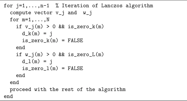
The idea is to add the following pseudo-code to the Lanczos algorithm (we assume to stop it at the (n−1)-th iteration).
First, initialize the variablesis_zero_k,is_zero_l,d_kandd_las follows
for i=1,...,N
is_zero_k(i) = TRUE is_zero_l(i) = TRUE
d_k(i) = n % vector of the distances from k
d_l(i) = n % vector of the distances to l
end
and then modify the method by adding the procedure below, to derive the distances from the nonzero pattern ofvj and wj, at each step of the scheme
for j=1,...,n-1 % Iteration of Lanczos algorithm
compute vector v_j and w_j
for m=1,...,N
if v_j(m) > 0 && is_zero_k(m) d_k(m) = j
is_zero_k(m) = FALSE end
if w_j(m) > 0 && is_zero_L(m) d_l(m) = j
is_zero_l(m) = FALSE end
end
proceed with the rest of the algorithm end
Notice that ifnis smaller or equal than the diameter of the graph, there can be null elements invjforj= 0, . . . , n−1. Nevertheless, for all these elements,nis a lower
bound for the distance, which can then be used to approximateδin Theorem5.3. On the other hand, let us remark that many real-world networks have a small diameter, thus we expect the proposed technique to be able to actually compute the desired distances in typical applications. Also note that by using this strategy, computing the diagonal off(A) allows to simultaneously address the all-pair shortest-path distances of the graph. This is particularly effective when dealing with undirected graphs. In that case, in fact, the entries f(A)kk can be computed with the Hermitian Lanczos
method which further ensures no breakdowns. Table 1 in the next section shows how this strategy behaves on four sample undirected networks, where the diagonal of the exponential function is approximated by the Hermitian Lanczos method and the number of maximal iterations varies.
[image:15.612.76.397.345.518.2]6. Numerical examples. In this section we illustrate the behavior of the pro-posed bounds on some example networks.
The first explanatory example graph we consider is represented in Figure1. The considered graphGis made by two simple cycles (closed undirected paths) with 111 nodes each, and by one directed edge→e from node 111 to node 112.
Fig. 1.Example: two cycles connected by a directed bridge(n, m)in which we add the edge in the opposite direction(m, n).
Since there are no closed walks passing through→e, all the nodes in G have the same f-centrality. The graph is then perturbed by the insertion of one single new directed edge←e from node 112 to node 111. This new edge “closes the two-directional bridge” between the two circles, resulting into a perturbation of thef-centrality scores of the nodes. In Figure2we plot in red crosses the values|exp(A)kk−exp(A)ekk|(left
plot) and those of |rα(A)kk−rα(A)e kk| with α = 3 (right plot), for k = 1, . . . ,222.
With blue circles, instead, we represent the bound in Corollaries 5.4(left plot) and 5.5 (right plot) for every admissiblek. As we can see the behavior of the decays of the differences is well approximated by the bounds. Moreover, we observe that the exponential decay for the exponential centrality variation as well the linear decay of the resolvent one are captured by the bound.
0 50 100 150 200
10-20 10-10 100
0 50 100 150 200
10-20 10-10 100
Fig. 2.In the ordinate: |f(A)kk−f(Ae)kk|(red crosses) when adding the edge ←
e in the graph of Figure1and the bounds (blue circles) of Corollaries5.4and5.5. In the abscissa: k, the nodes of the graph. From left to right: variation of exponential centrality f(x) = exp(x); variation of resolvent centralityf(x) =r3(x).
In the following we present four examples of real-world undirected networks whose diameter is proportional to the logarithm of the number of nodes. Our analysis is meant to show the correlation between the variation of the network centralities and the variation of the distances in Gwith respect to the set of perturbed edges. For
[image:16.612.150.360.176.281.2] [image:16.612.89.425.475.584.2]this reason, normalized adjacency matricesA are considered below, so to guarantee the field of values of both the original and the perturbed matrices to be constrained within the unit segment [−1,1].
The considered network data are borrowed from [16,33] and are briefly described below:
Gnutella A snapshots of the Gnutella peer-to-peer file sharing network in August, 8, 2002. Nodes represent hosts in the Gnutella network topology and edges represent connections between the Gnutella hosts. Number of nodes: 6300, Number of edges: 41297, Diameter: 10;
Facebook This dataset consists of anonymous “friends circles” from Facebook. Face-book data was collected from survey participants. Number of nodes: 4038, Number of edges: 176167, Diameter: 10;
GRCQ General Relativity and Quantum Cosmology (GR-QC) collaboration net-work. Data are collected from the e-print arXiv and covers scientific collab-orations between authors papers submitted to GR-QC category. The data covers papers in the period from January 1993 to April 2003. Number of nodes: 5242, Number of Edges: 14496, Diameter: 17;
Erd¨os Erd¨os collaboration network. Number of nodes: 472, Number of edges: 2628, Diameter: 11.
For each network we compute (approximate) the exponential centrality index exp(A)kk, k= 1, . . . , n, by runningn iterations of the Lanczos algorithm. By using
the method presented in Subsection 5.4, for every ` we can compute dn(k, `): an
approximation of dG(k, `). If dG(k, `) ≤ n, then dn(k, `) = dG(k, `). Otherwise, if d(k, `)> nthendn(k, `) =n≤dG(k, `).
We compared the proposed methods withdM(k, `): the distance between kand ` computed by the Matlab function distances. Note that, dM(k, k) = 0 for every
node k, whereas dn(k, k) is eithern or the minimal length of a closed walk passing
throughk. Moreover, whenkand` are disconnected,dn(k, `) =nfor everyn, while
distancescorrectly sets to∞the distance between disconnected nodes. In order to evaluate the proposed method, we consider the quantity
%n(G) =
#{(k, `)|dn(k, `)6=dM(k, `), k6=`,dG(k, `)<∞}
#{(k, `)|k6=`,dG(k, `)<∞} ,
which depends on the number of pairs (k, `) for whichdn(k, `)6=dM(k, `) (excluding
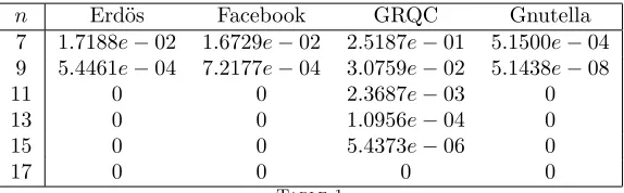
the disconnected and the coincident nodes). Table1presents%n(G) for some values of
nand for the networks listed above. The table clearly shows that for a small number of Lanczos iterations we are able to determine most of the distances. Moreover, whenn is greater or equal to the diameter of the network we always havedn(k, `) =dM(k, `),
for everyk6=`anddG(k, `)<∞.
Now, for each network, we select the 10 nodes having smallest centrality exp(A)kk
and we perturb the edge topology of the graph by adding all the missing edges among those nodes (obtaining a clique connecting all the “less important” nodes).
The plots of Figure 3 represent the actual variation of network exp-centrality values|exp(A)kk−exp(A)ekk|(red crosses) and the bound in Corollary5.4(blue circle).
Let us point out that in the plots shown, we are relabeling the nodes according with the distance from (and to) the setSof modified nodes: the larger is the node indexkthe fartherkis fromS. The results show that the proposed bounds, although not tight, well approximate the actual behavior of the variation off(A)kk. This allows to predict
the nodes whose centrality index remains effectively unchanged under perturbations
n Erd¨os Facebook GRQC Gnutella 7 1.7188e−02 1.6729e−02 2.5187e−01 5.1500e−04 9 5.4461e−04 7.2177e−04 3.0759e−02 5.1438e−08
11 0 0 2.3687e−03 0
13 0 0 1.0956e−04 0
15 0 0 5.4373e−06 0
17 0 0 0 0
[image:18.612.114.401.95.184.2]Table 1
Values of%n(G)forn= 7,9,11,13,15,17and for the networks: Erd¨os, Facebook, GRQC, and
Gnutella.
of the original graph topology. For example, the exp-centrality of all the nodes from 3000 onwards in GRQC is guaranteed to be unchanged up to 10 digits of precision.
100 200 300 400
10-20 10-10 100
Er
dös
1000 2000 3000 4000
10-20 10-10 100
F
acebook
1000 2000 3000 4000 5000 10-20
10-10 100
GRQC
1000 2000 3000 4000 5000 6000 10-20
10-10 100
Gnut
ella
Fig. 3.Absolute variation|exp(A)kk−exp(Ae)kk|whenkranges from1toN. The perturbed
edges areδE =S×S, whereSis the set of 10nodes with leastexp-centrality. Nodes in the plot are ordered so that the larger iskthe farther it is fromS. Red crosses show the actual difference whereas the blue circles show the bound of Corollary5.4.
7. Conclusion. Centrality and communicability indices based on function of matrices are among the most effective measures of the importance of nodes and of the robustness of edges in a network. These quantities are defined as the entriesf(A)k`
where f(A) is a suitable function of a matrixA describing the structure of the net-work G. In this work we address the somewhat natural problem of understanding the stability of such indices with respect to perturbations in the edge topology of the graph. Our analysis reveals that the absolute variation of f(A)k` decays
exponen-tially with respect to the distance inGthat separateskand `from the set of nodes touched by the perturbed edges. The knowledge of this behavior can be of help in several practical applications. In fact, ifAis modified intoAe=A+δA, the entries of
f(A) should in principle be re-computed from scratch. However, we propose a simplee
numerical strategy that allows to compute the distances between nodes in G
[image:18.612.89.422.274.482.2]taneously with the computation of the entries off(A), with essentially no additional cost. In particular, computing the diagonal off(A) for undirected networks (the net-work f-centrality scores) allows to compute the all-pairs shortest-path distances in the graph. Thus, using the proposed bounds, we are able to predict the magnitude of variation in the f-centralities ofGwhen changes occur in a localized set of edges or, viceversa, for each nodek we can locate a set of nodes whose change in the edge topology affects the scoref(A)kk by a small order of magnitude.
Examples of application include the case where the edge topology is evolving in time and changes inGhappen more frequently in network subareas being peripheral with respect to the subset of nodes one is actually interested in, or where the infor-mation on the edge structure of peripheral nodes is not fully reliable or, equivalently, is likely to be affected by noise.
Finally, the results proposed are numerically tested on some example networks borrowed from real-world applications. Our experiments show that the proposed bounds well resemble the actual behavior of the variation off(A)k` although being
some orders of magnitude larger. A clear margin for improvements and further work is thus left open to determine a better constantc >2 to be added in the exponent δ+c of Theorem5.3.
REFERENCES
[1] U. Alon, An introduction to systems biology: design principles of biological circuits, CRC press, 2006.
[2] M. Aprahamian, D. J. Higham, and N. J. Higham,Matching exponential-based and resolvent-based centrality measures, Journal of Complex Networks, (2015), p. cnv016.
[3] A.-L. Barab´asi and R. Albert, Emergence of scaling in random networks, Science, 286
(1999), pp. 509–512.
[4] B. Beckermann,Image num´erique, GMRES et polynˆomes de Faber, C. R. Math. Acad. Sci. Paris, 340 (2005), pp. 855–860.
[5] M. Benzi and P. Boito,Quadrature rule-based bounds for functions of adjacency matrices, Linear Algebra and its Applications, 433 (2010), pp. 637–652.
[6] ,Decay properties for functions of matrices overC∗-algebras, Linear Algebra Appl., 456 (2014), pp. 174–198.
[7] M. Benzi, E. Estrada, and C. Klymko,Ranking hubs and authorities using matrix functions, Linear Algebra and its Applications, 438 (2013), pp. 2447–2474.
[8] M. Benzi and N. Razouk,Decay bounds and O(n) algorithms for approximating functions of sparse matrices, Electron. Trans. Numer. Anal., 28 (2007), pp. 16–39.
[9] M. Benzi and V. Simoncini,Decay Bounds for Functions of Hermitian Matrices with Banded or Kronecker Structure, SIAM J. Matrix Anal. Appl., 36 (2015), pp. 1263–1282.
[10] S. Boccaletti, V. Latora, Y. Moreno, M. Chavez, and D.-U. Hwang,Complex networks: Structure and dynamics, Physics reports, 424 (2006), pp. 175–308.
[11] P. Bonacich,Power and centrality: A family of measures, American journal of sociology, 92 (1987), pp. 1170–1182.
[12] U. Brandes and T. Erlebach, eds.,Network analysis: methodological foundations, vol. 3418, Springer Science & Business Media, 2005.
[13] S. Brin and L. Page,The anatomy of a large-scale hypertextual web search engine, Computer
networks and ISDN systems, 30 (1998), pp. 107–117.
[14] F. Chung and R. Graham,Quasi-random graphs with given degree sequences, Random Struc-tures & Algorithms, 32 (2008), pp. 1–19.
[15] J. J. Crofts and D. J. Higham,A weighted communicability measure applied to complex brain networks, Journal of the Royal Society Interface, (2009), pp. rsif–2008.
[16] T. Davis and Y. Hu,University of Florida sparse matrix collection, ACM Transactions on Mathematical Software, 38 (2011), pp. 1–25.
[17] E. Estrada and M. Benzi,Core–satellite graphs: Clustering, assortativity and spectral prop-erties, Linear Algebra and its Applications, 517 (2017), pp. 30–52.
[18] E. Estrada and D. J. Higham,Network properties revealed through matrix functions, SIAM review, 52 (2010), pp. 696–714.
[19] E. Estrada and J. A. Rodriguez-Velazquez,Subgraph centrality in complex networks, Phys-ical Review E, 71 (2005), p. 056103.
[20] D. Fasino and F. Tudisco,An algebraic analysis of the graph modularity, SIAM Journal on Matrix Analysis and Applications, 35 (2014), pp. 997–1018.
[21] , Generalized modularity matrices, Linear Algebra and its Applications, 502 (2016), pp. 327–345.
[22] C. Fenu, D. Martin, L. Reichel, and G. Rodriguez,Block Gauss and Anti-Gauss Quadra-ture with Application to Networks, SIAM Journal on Matrix Analysis and Applications, 34 (2013), pp. 1655–1684.
[23] L. C. Freeman, Centrality in social networks conceptual clarification, Social networks, 1 (1978), pp. 215–239.
[24] G. H. Golub and G. Meurant,Matrices, Moments and Quadrature with Applications,
Prince-ton Series in Applied Mathematics, PrincePrince-ton University Press, 2009.
[25] G. H. Golub and C. F. Van Loan,Matrix computations, vol. 3, JHU Press, 2012.
[26] P. Grindrod and D. J. Higham,A dynamical systems view of network centrality, Proc. Royal Society A, 470 (2014), p. 20130835.
[27] P. Grindrod and M. Kibble,Review of uses of network and graph theory concepts within proteomics, Expert review of proteomics, 1 (2004), pp. 229–238.
[28] N. J. Higham,Functions of matrices: theory and computation, SIAM, 2008.
[29] K. Kloster,Graph diffusions and matrix functions: Fast algorithms and localization results, PhD thesis, Purdue University, 2016.
[30] C. Lanczos,An iterative method for the solution of the eigenvalue problem of linear differential and integral operators, J. Res. Natl. Bur. Stand., 45 (1950), pp. 255–282.
[31] C. Lanczos,Solution of systems of linear equations by minimized iterations, J. Res. Natl. Bur. Stand., 49 (1952), pp. 33–53.
[32] A. N. Langville and C. D. Meyer,Who’s# 1?: the science of rating and ranking, Princeton University Press, 2012.
[33] J. Leskovec and A. Krevl,SNAP Datasets: Stanford Large Network Dataset Collection.
http://snap.stanford.edu/data, June 2014.
[34] C.-K. Li, B.-S. Tam, and P. Wu,The numerical range of a nonnegative matrix, Linear algebra and its applications, 350 (2002), pp. 1–23.
[35] J. Maroulas, P. Psarrakos, and M. Tsatsomeros, Perron–Frobenius type results on the numerical range, Linear algebra and its applications, 348 (2002), pp. 49–62.
[36] P. Mercado, F. Tudisco, and M. Hein,Clustering Signed Networks with the Geometric Mean of Laplacians, in Advances in Neural Information Processing Systems, 2016, pp. 4421–4429. [37] J. L. Morrison, R. Breitling, D. J. Higham, and D. R. Gilbert,A lock-and-key model for
protein–protein interactions, Bioinformatics, 22 (2006), pp. 2012–2019.
[38] M. E. J. Newman,Finding community structure in networks using the eigenvectors of matri-ces, Physical review E, 74 (2006), p. 036104.
[39] A. Y. Ng, M. I. Jordan, and Y. Weiss,On spectral clustering: Analysis and an algorithm, in Advances in Neural Information Processing Systems (NIPS), vol. 14, 2001, pp. 849–856. [40] J.-P. Onnela, J. Saram¨aki, J. Hyv¨onen, G. Szab´o, D. Lazer, K. Kaski, J. Kert´esz, and A.-L. Barab´asi,Structure and tie strengths in mobile communication networks,
Proceed-ings of the National Academy of Sciences (PNAS), 104 (2007), pp. 7332–7336.
[41] S. Pozza, M. Pranic, and Z. Strakoˇs,Lanczos algorithm and the complex Gauss quadrature. 2017.
[42] S. Pozza and V. Simoncini,Decay bounds for non-Hermitian matrix functions, submitted, arXiv:1605.01595v3 [math.NA], (2016).
[43] K. Rohe, S. Chatterjee, and B. Yu,Spectral clustering and the high-dimensional stochastic blockmodel, The Annals of Statistics, (2011), pp. 1878–1915.
[44] P. K. Suetin,Series of Faber polynomials, Gordon and Breach Science Publishers, 1998. [45] H. C. Thomas, C. E. Leiserson, R. L. Rivest, and C. Stein,Introduction to algorithms,
vol. 6, MIT press Cambridge, 2001.
[46] U. Von Luxburg, A tutorial on spectral clustering, Statistics and computing, 17 (2007), pp. 395–416.
[47] J. Wilkinson,The algebraic eigenvalue problem, vol. 87, Clarendon Press Oxford, 1965.