Optimisation of arbitrary light beam generation with spatial light modulators

Optimisation of arbitrary light beam generation

with spatial light modulators

Neal Radwell1*, Rachel F. Offer2, Adam Selyem1 and Sonja Franke-Arnold1

1_{School of Physics and Astronomy, SUPA, University of Glasgow, Glasgow, G12}

8QQ, UK

2_{Department of Physics, SUPA, University of Strathclyde, Glasgow G4 0NG, UK}

E-mail: ∗_{[email protected]}

Abstract. Phase only spatial light modulators (SLMs) have become the tool of

choice for shaped light generation, allowing the creation of arbitrary amplitude and phase patterns. These patterns are generated using digital holograms and are useful

for a wide range of applications as well as for fundamental research. There have

been many proposed methods for optimal generation of the digital holograms, all of which perform well under ideal conditions. Here we test a range of these methods under specific experimental constraints, by varying grating period, filter size, hologram resolution, number of phase levels, phase throw and phase nonlinearity. We model beam generation accuracy and efficiency and show that our results are not limited to the specific beam shapes, but should hold for general beam shaping. Our aim is to demonstrate how to optimise and improve the performance of phase-only SLMs for experimentally relevant implementations.

1. Introduction

Light is an essential tool in a wide array of modern day applications from microscopy to laser machining. Manipulating and controlling light therefore has been the focus of much attention over the last several hundred years. This control has traditionally been achieved with lenses and other fixed optical components, however in the modern era, an even greater level of control can be obtained using dynamic components such as spatial light modulators (SLMs) [1] and digital micromirror devices (DMDs). These computer controlled devices can be programmed to generate almost any beam imaginable and are now essential in a wide array of applications [2] including optical tweezers [3, 4, 5], microscopy [6, 7], nanofibre mode coupling,[8], quantum information and imaging [9, 10, 11], coherence tuning [12], super-resolution imaging [13] and atom trapping and memories [14, 15, 16].

testing their ability to recreate the desired intensity distribution, and indirectly testing their phase by monitoring propagation. While that work was performed under optimum conditions for our SLM device, many experiments are performed under restraints dictated by the available device and methodology. Here we use numerical simulations to test a range of beam generation methods under several, experimentally relevant, non-ideal circumstances. Furthermore the evaluation of a complex fidelity parameter allows us to explicitly assess both the intensity and phase fidelity of each method.

There are many approaches to beam shaping using phase modulation, including multiple phase-holograms [18], iterative techniques [19, 20, 21] and the use of DMDs [22, 23], however here we concentrate on beam shaping using a single phase-only SLM, using non-iterative hologram generation techniques.

This paper begins with a summary of the beam generation techniques, followed by an overview of the numerical method and definition of our quality metrics. The main section outlines each variable or limitation to be considered and then presents our results for beam accuracy, efficiency and composite quality (the power in the desired mode), before drawing conclusions.

2. Numerical methods

The phase-only digital hologram generation methods considered in this work are based on single-pass digital holograms, using diffraction from phase gratings to allow amplitude

and phase control. The first six methods, labelled A-F, are outlined in detail in

[17], following the same labelling. Method A is a naive approach which simply uses the amplitude of the desired beam to control the grating depth, and therefore shape the diffracted light intensity [17]. Method B uses a method inspired by the original holography work by Gabor et al. [24] which interferes the input and desired fields and uses the phase of the resulting field as the hologram. Method C modulates the grating depth, in a similar way to method A, however uses a more rigorous analysis of the relationship between grating depth and field amplitude [25]. Method D is an adjustment to method C, suggested by Bolduc et at. [26] to account for an extra phase term. Methods E and F again use a more rigorous approach to link the grating depth and the desired intensity but find solutions involving sine functions, details of which can be found in [27]. In addition to these, we test a further method based on pseudo-random encoding, which we label Method G, and was suggested in [28]. This method achieves amplitude modulation by inducing a randomly sampled phase error whose variance is related to the desired amplitude.

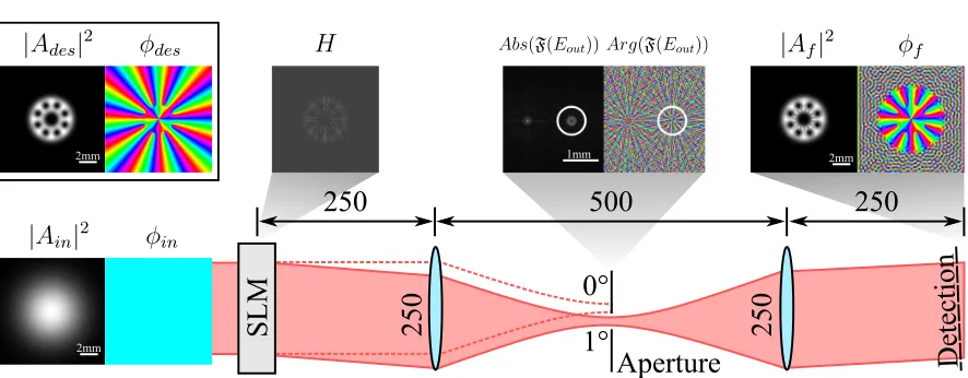
Our simulation methodology is outlined schematically in Figure 1. We begin with

an input beamEin(x, y) =Ain(x, y) exp(iφin(x, y)), which we model as a Gaussian beam

with 1/e2 _{waist size of 4.65 mm, chosen to represent a realistic beam size for common}

SLM sizes of around 10 mm. A hologramH(x, y) is then generated from the input beam

and our desired beam Edes(x, y) = Ades(x, y) exp(iφdes(x, y)) using one of the methods

SLM

250

Aperture

250

Detection

250

500

250

2mm 1mm 2mm

2mm

0°

1°

Figure 1. Summary of numerical method. The input beam and desired beam are

defined to generate the hologram H. This phase is added to the input beam and the output beam is Fourier transformed and filtered. The beam undergoes an inverse Fourier transform to produce the final beam which is then compared to the desired beam. Distances and focal lengths are given in millimeters.

a fundamental Gaussian, a single Laguerre-Gaussian mode (LG10,0), a superposition

of LG modes known as an optical Ferris wheel [29] and a non-propagating field with intensity shaped as a ‘Laser class’ sailboat, and phase in the shape of a dog. The three

laser modes all have a desired beam waist of 0.9 mm 1/e2 _radius.

The effect of the hologram is to generate an output beam after the SLM of

Eout(x, y) = Ein(x, y)eiH(x,y). (1)

In an experiment, this beam would be passed through an aperture in the Fourier plane of the SLM to remove unwanted diffraction orders. We model this by taking the

2D Fourier transform ofEout(x, y) and multiplying by a filtering function. We filter using

a binary circular mask, centred on the position of the first diffraction order. The inverse

2D Fourier transform then returns the final fieldEf(x, y) =Af(x, y) exp(iφf(x, y)) at the

detection plane. This field includes the phase tilt imposed by the grating and therefore we subtract this phase tilt for comparison with the desired beam, equivalent to tilting our detection plane to be perpendicular to the propagation direction of the first order diffracted beam.

To gauge the quality ofEf we use three metrics, the accuracy ofEf in comparison

toEdes, the conversion efficiency and the compound quality. The accuracy is determined

by the complex fidelity [30]

F =

1

N

Z

Edes(x, y)Ef∗(x, y)dxdy

2

, (2)

where N = qR

|Edes(x, y)|2dxdy×

R

|Ef(x, y)|2dxdy is a normalisation function

and the limits of the integrals are given by the grid we choose to calculate on. We

simulate our beams on a dense grid of 2400×2400 points, representing a physical size of

calcuated at the reduced resolution of 600×600 and upscaled to 2400×2400 without

interpolation, unless otherwise stated. In general F is very close to 1, and to improve

clarity we plot our data logarithmically as −log₁₀(1−F).

The efficiency Pef f is calculated by comparing the power in Ef and Ein using

Pef f =

R

|Ef(x, y)|2dxdy

R

|Ein(x, y)|2dxdy

, (3)

and the compound quality is simply the product of the quality and efficiency, which can be considered to be a measure of the amount of power in the desired mode. The compound quality can be useful to gauge the relative performance of the different methods, though depending on the chosen application, accuracy or efficiency alone may be a better metric.

3. Results

In this work we are interested in how the accuracy and efficiency of the beam generation

methods vary with certain experimentally relevant parameters. We first test the

perfomance of the methods when generating beams of varying spatial complexity, in order to be confident that the later results are not a special case for the chosen beam shapes, and hold for any general beam. We then explore the role of the grating period and Fourier filter size before considering further experimentally relevant constraints. There are several different SLM models on the market with a range of technical specifications, and we explore the effect of varying a number of these specifications: pixel number, number of grey levels, phase throw and phase response. Unless otherwise noted, the default values for the simulation are as follows: grating period 5 pixels (20

when upscaled to 2400×2400), aperture radius 300µm, hologram resolution 600×600px,

hologram size 12 mm×12 mm, grid size 2400×2400, grey levels 256, phase throw 2π

and ideal linear phase response.

3.1. Modal Dependence

The accuracy and efficiency of all methods may be dependent on the shape of the desired field. In order to test all possible beam shapes, we can gauge the performance of each method while generating all modes of a complete, orthogonal basis. We choose the modes of the Hermite-Gaussian (HG) basis, which are parameterised by their mode

order numbers n and m. As n and m are increased, the modes become more intricate,

with higher spatial frequency components. By testing the performance of the generation

methods across a range of HG modes of increasing n and m we can therefore test the

performance of the methods for any general beam. To fully map this basis, an infinite

number of measurements are required, however here we chose a sub-set ofm, n <20 for

practical reasons.

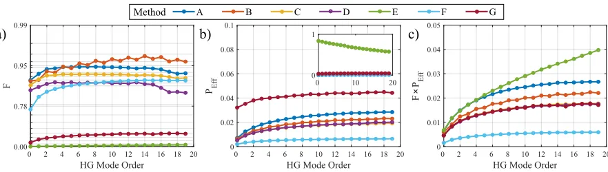
The results are shown in Figure 2 and show some general trends: the accuracy

HG Mode Order

0 2 4 6 8 10 12 14 16 18 20

F

0.00 0.78 0.95 0.99

HG Mode Order

0 2 4 6 8 10 12 14 16 18 20 PEff

0 0.02 0.04 0.06 0.08 0.1

0 10 20

0 1

HG Mode Order

0 2 4 6 8 10 12 14 16 18 20

F

PEff

0 0.01 0.02 0.03 0.04 0.05

a) b) c)

A B C D E F G

Method

Figure 2. Measurements in a modal basis. a) Beam generation accuracy, plotted on

a log scale, b) absolute efficiency and c) composite quality results of methods A-G generating a range of Hermite-Gaussian modes. The main graphs are zooms to show detail while the insets (if present) show the overall data.

seems to show some decrease in quality for higher m, n. The efficiency is increasing

slightly for higher values of m, n and this can be attributed to the increased spatial

overlap between the input beam (Gaussian with 4.65 mm beam waist) and the desired

modes (all with beam waist 400µm). The main result however is that there is very

little overlap of the results for separate methods, illustrating that there is no strong spatial dependence on the relative performance of the methods. This shows that the performance of the methods should not be strongly dependent on the exact form of the desired beam, and therefore the results shown in later sections should hold for general beams.

3.2. Grating Period

All tested methods rely on diffraction from a grating to provide amplitude shaping

and increased mode purity. When choosing the grating period there is a tradeoff;

short periods increase the separation between the desired mode and the background light in the Fourier plane, improving the spatial filtering and therefore mode quality, whereas long grating periods have more ideal phase profiles which improves efficiency. For simplicity we test grating periods with integer numbers of pixels per period and the results are shown in Figure 3.

A B C D E F G Method

a) b) c)

Grating Period (px)

0 5 10 15 20 25 30

F

0.00 0.54 0.78 0.90

Grating Period (px)

0 5 10 15 20 25 30

PEff

0 0.05 0.1 0.15 0.2 0.25 0.3

Grating Period (px)

0 5 10 15 20 25 30

F

PEff

0 0.05 0.1 0.15 0.2

F

0.90 0.99 0.999 0.9999

PEff

0.1 0.2 0.3 0.4 0.5 0.6

F

PEff

0.1 0.2 0.3 0.4

F

0.90 0.99 0.999 0.9999

PEff

0.1 0.2 0.3 0.4 0.5 0.6

F

PEff

0.1 0.2 0.3 0.4

F

0.90 0.99 0.999 0.9999

PEff

0.2 0.4 0.6 0.8

F

PEff

0.02 0.04 0.06 0.08 0.1

Figure 3. Grating period results. Grating periods are stated before hologram

upscaling to 2400×2400. a) Beam generation accuracy, plotted on a log scale, b)

absolute efficiency and c) composite quality results of methods A-G generating the desired beam shown on left.

A B C D E F G

Method

a) b) c)

Aperture Size (mm)

0.1 0.4 0.7 1

F

0.00 0.68 0.90 0.97

Aperture Size (mm)

0.1 0.4 0.7 1

PEff 0 0.05 0.1 0.15 0.2

Aperture Size (mm)

0.1 0.4 0.7 1

F PEff 0 0.05 0.1 0.15 0.2 F 0.90 0.99 0.999 0.9999 PEff 0.1 0.2 0.3 0.4 0.5 F PEff 0.1 0.2 0.3 0.4 F 0.90 0.99 0.999 0.9999 PEff 0.1 0.2 0.3 0.4 0.5 F PEff 0.1 0.2 0.3 0.4 F 0.90 0.99 0.999 0.9999 PEff 0.02 0.04 0.06 0.08 0.1 0.12

0.1 0.5 1

0 1 F PEff 0.02 0.04 0.06 0.08 0.1

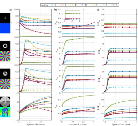
Figure 4. Aperture size results. a) Beam generation accuracy, plotted on a log scale,

b) absolute efficiency and c) composite quality results of methods A-G generating the desired beam shown on left. The main graphs are zooms to show detail while the insets (if present) show the overall data.

3.3. Aperture Size

The effect of the grating is to separate the desired beam from the background light in the far-field. An aperture, centred on the correct diffraction order, is used to remove all unmodulated light contributions. In reality however the diffracted spots are spatially extended with some overlap that depends on the spatial frequencies present in the desired pattern. The ideal aperture will be small enough to block out all background light, and yet large enough to avoid filtering of high spatial frequencies. This is demonstrated in column a) of Fig. Figure 4 by the position of the peak for the different beam profiles.

The LG beam and the optical ferris wheel contain only a few higher spatial frequency components which are blocked for the lowest filter sizes, and the more intricate spatial structure of the sailboat results in the increase of performance with aperture size.

Ideally, each method would separate the desired field from the background field perfectly. In reality each method separates the desired and background fields differently. Methods A to F achieve this by concentrating the background light in the zero diffraction order. Instead method G randomly distributes the background field. This random spreading means that the background light increases proportional to the area of the filter, leading to poor fidelity for large filter sizes compared to all of the other methods. Interestingly, the compound efficiency shown in Figure 4(c) shows that each method performs similarly, suggesting that one can trade beam accuracy for efficiency simply by altering the filter size. This may be useful for applications requiring either maximum accuracy or efficiency at the expense of the other.

3.4. SLM Resolution

A digital hologram is an approximate, pixelated version of a continuous phase hologram, with greater pixel numbers leading to a better approximation. Pixel number is restricted by the physical resolution of the SLM and here we test the accuracy and efficiency of each

method while varying the pixel resolution. Each hologram is a square n×n hologram

withnbeing the resolution, with the physical size of the hologram fixed at 12×12mm and

the grating pixel period altered to keep the physical grating period constant (600µm).

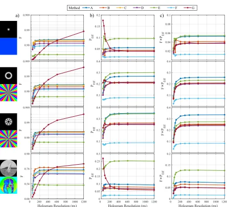
The results are shown in Figure 5 and as expected, holograms defined with fewer pixels produce beams with lower accuracy and efficiency simply because the pixelated phase is not a good representation of the ideal phase. The increase in accuracy and efficiency

however starts to level off at modest pixel numbers of around 200×200 pixels, suggesting

that large numbers of pixels may not readily translate to large performance increases. Method G again shows noteworthy behaviour, with an accuracy that rises sharply with hologram resolution. This can be attributed to the statistical nature of the method, indeed the authors of [28] describe the method as the realisation of the ’rule of large numbers’.

3.5. Grey levels

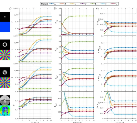
In addition to pixelation, a real SLM will also discretise the desired phase, with modern SLMs typically having 256 or more distinct phase levels. Here we investigate the importance of this fine control by adjusting the number of distinct phase levels represented in the hologram. This is achieved by calculating the exact phase of the ideal hologram (to 32bit computer precision) and digitising into a specific number of phase (grey) levels. We characterise the phase resolution in terms of ’bit depth’, where

2b discrete phase levels have a bit depth ofb. The data in Figure 6 shows that the result

A B C D E F G Method

a) b) c)

Hologram Resolution (px) 0 200 400 600 800 1000 1200

F

0.00 0.54 0.78 0.90

Hologram Resolution (px) 0 200 400 600 800 1000 1200 PEff

0 0.05 0.1 0.15 0.2 0.25 0.3

Hologram Resolution (px) 0 200 400 600 800 1000 1200

F

PEff

0 0.05 0.1 0.15 0.2

F

0.90 0.99 0.999

PEff

0.1 0.2 0.3 0.4

F

PEff

0.1 0.2 0.3 0.4

F

0.90 0.99 0.999

PEff

0.1 0.2 0.3 0.4

F

PEff

0.1 0.2 0.3 0.4

F

0.90 0.99 0.999

PEff

0.05 0.1 0.15 0.2

F

PEff

0.02 0.04 0.06 0.08 0.1

Figure 5. Pixel number results. a) Beam generation accuracy, plotted on a log scale,

b) absolute efficiency and c) composite quality results of methods A-G generating the desired beam shown on left.

a bit depth of 3. Conversely, methods C and F have the best ultimate performance at high bit depths, with performance only levelling off at a bit depth of 7. The results therefore suggest that systems with low bit depths would benefit from methods D and G, whereas systems capable of higher bit depths achieve best results using methods C and F. The efficiency performance is more straight forward, with all methods achieving near peak efficiency at a bit depth of 4.

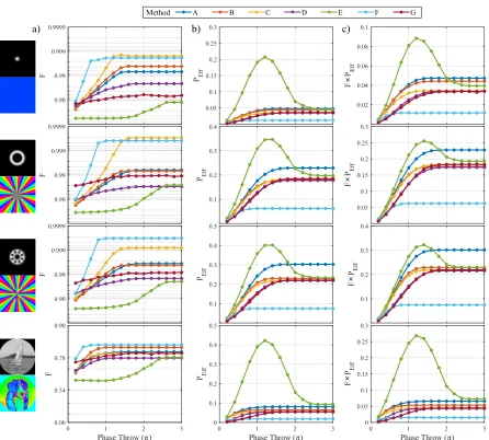
3.6. Phase Throw

Ideally one would use an SLM capable of full 2π phase modulation at the desired

wavelength, however if using an SLM designed for a shorter wavelength, or a cheaper model, this may not be possible. In Figure 7 we show the performance of the different

A B C D E F G

Method

a) b) c)

Bit Depth

1 2 3 4 5 6 7 8 9 10

F

0.00 0.54 0.78 0.90

Bit Depth

1 2 3 4 5 6 7 8 9 10 PEff

0 0.05 0.1 0.15 0.2

Bit Depth

1 2 3 4 5 6 7 8 9 10

F

PEff

0 0.02 0.04 0.06 0.08 0.1

F

0.90 0.99 0.999 0.9999

PEff

0.1 0.2 0.3 0.4 0.5

F

PEff

0.1 0.2 0.3 0.4

F

0.90 0.99 0.999 0.9999

PEff

0.1 0.2 0.3 0.4 0.5

F

PEff

0.1 0.2 0.3 0.4

F

0.90 0.99 0.999 0.9999

PEff

0.2 0.4 0.6 0.8

F

PEff

0.02 0.04 0.06 0.08 0.1

Figure 6. Bit depth results. a) Beam generation accuracy, plotted on a log scale,

b) absolute efficiency and c) composite quality results of methods A-G generating the desired beam shown on left.

generated with a full 2π phase range before reducing the phase range not by simply

scaling the phase uniformly down, but preserving the gradient of the phase as much as possible using a method initially suggested in [31]. The results show the expected general trend towards increasing efficiency and accuracy for increasing phase depth. The accuracy results show that all methods except method E reach peak performance before

2π. Noteworthy is the performance of method F, which reaches peak accuracy with only

π phase modulation, making it ideal for use with devices with reduced phase throw.

The efficiency results demonstrate the real strength of method E, which is designed to achieve peak performance at reduced phase throws. The peak should appear around

the first minimum of the Bessel function of the first kind at 1.16π and indeed the results

show that the method achieves peak efficiency at 1.2π. It is worth noting at this stage

A B C D E F G

Method

Phase Throw ( )

0 1 2 3

F

0.00 0.54 0.78 0.90

Phase Throw ( )

0 1 2 3

PEff 0 0.1 0.2 0.3 0.4 0.5

Phase Throw ( )

0 1 2 3

F PEff 0 0.05 0.1 0.15 0.2 0.25 0.3 F 0.90 0.99 0.999 0.9999 PEff 0.1 0.2 0.3 0.4 0.5 F PEff 0.1 0.2 0.3 0.4 F 0.90 0.99 0.999 0.9999 PEff 0.1 0.2 0.3 0.4 F PEff 0.05 0.1 0.15 0.2 0.25 0.3 F 0.90 0.99 0.999 0.9999 PEff 0.05 0.1 0.15 0.2 0.25 0.3 F PEff 0.02 0.04 0.06 0.08 0.1

π π π

a) b) c)

Figure 7. Phase throw results. a) Beam generation accuracy, plotted on a log scale,

b) absolute efficiency and c) composite quality results of methods A-G generating the desired beam shown on left.

comprise few modal components, i.e. the fundamental Gaussian, LG beam and Ferris wheel, but comparable to other methods for the more complicated image of the sailboat.

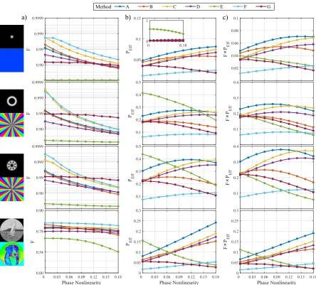
3.7. Nonlinear Phase Response

A B C D E F G

Method

a) b) c)

Phase Nonlinearity 0 0.03 0.06 0.09 0.12 0.15 0.18

F 0.00 0.54 0.78 0.90 Phase Nonlinearity 0 0.03 0.06 0.09 0.12 0.15 0.18 PEff 0 0.05 0.1 0.15 0.2 0.25 0.3 Phase Nonlinearity 0 0.03 0.06 0.09 0.12 0.15 0.18

F PEff 0 0.05 0.1 0.15 0.2 0.25 0.3 F 0.90 0.99 0.999 0.9999 PEff 0.1 0.2 0.3 0.4 0.5 F PEff 0.1 0.2 0.3 0.4 F 0.90 0.99 0.999 0.9999 PEff 0.1 0.2 0.3 0.4 0.5 F PEff 0.1 0.2 0.3 0.4 F 0.90 0.99 0.999 0.9999 PEff 0.05 0.1 0.15

0 0.18

0 1 F PEff 0.02 0.04 0.06 0.08 0.1

Figure 8. Phase response results. a) Beam generation accuracy, plotted on a log scale,

b) absolute efficiency and c) composite quality results of methods A-G generating the desired beam shown on left. The main graphs are zooms to show detail while the insets (if present) show the overall data.

evenly spaced points on a straight line in the range 0-1 on both axes. The second and fourth points are then displaced down and up by the ’phase nonlinearity’ factor. For each set of points, the phase repsonse is recovered by fitting a cubic function through

the points and multiplying both axes by 2π. These shapes were phenomenologically

chosen to match the typical phase responses we have measured for SLM devices from a range of manufacturers.

the phase induced by the nonlinearity means that the grating is no longer directing all light with the same angle, but rather has a spread of angles. This can divert unwanted background light through the aperture, increasing the apparent efficiency, at the loss of some accuracy. In any case, this information could be used to maximise the power of a desired mode, albeit at the expense of beam accuracy.

More generally, until now, the five previous test criteria (grating period, filter size, resolution, grey levels, phase throw) have had minimal impact on the accuracy of the beam, indicating that the grating itself is very robust against all sorts of restrictions and it is only the efficiency which suffers due to limited overlap with the ideal phase. Here however, we see that the accuracy is strongly affected because the grating has become warped through the inaccurate phase mapping, and the efficiency remains high or even increases, in stark contrast to the previous results.

4. Conclusions

We have shown how the performance of several digital hologram generation methods compares when certain experimentally relevant parameters are varied. We find that the methods are largely spatial mode invariant, and hold for general beams. We find that for our experimentally realistic test parameters, grating periods between 5 and 15 pixels produce optimum results and that method G is only weakly dependent on period. Altering the Fourier filter size was found to trade accuracy for efficiency, which may prove useful in applications where either parameter needs to be maximised. The number of unique phase levels present in the hologram was found to vary strongly with each method, with ultimate performance of method G being reached for as few as 8 levels. Furthermore, near peak efficiency is reached for all methods with only 16 phase levels. Our test parameters also reveal that for all but method G, large pixel

numbers have little impact on beam accuracy, with as few as 200×200 pixels reaching

very high performance levels, however efficiency continues to increase for large pixel numbers. Again, method G stands out, and as the manifestation of the rule of large numbers, performs extremely well with large pixel numbers. The available phase throw

is optimally 2π and we find that efficiency is indeed maximised for 2π, but recognise

that method F provides excellent results with only π phase modulation. A reduction

in phase throw also emphasises the benefits of method E, where it achieves optimum

performance at 1.2π. The nonlinear phase response inherent in real SLM devices was

Funding Information

We acknowledge the financial support given by the Leverhulme Trust via project RPG-2013-386.

Acknowledgments

The authors would like to thank Johannes Courtial for providing access to the

WaveTracedevelopment library, a large collection of LabVIEW VIs specifically designed

for scalar optical modelling. We would also like to thank David Philips for insightful and useful discussions.

Bibliography

[1] Andrew Forbes, Angela Dudley, and Melanie McLaren. Creation and detection of optical modes

with spatial light modulators. Advances in Optics and Photonics, 8(2):200–227, 2016.

[2] Halina Rubinsztein-Dunlop, Andrew Forbes, MV Berry, MR Dennis, David L Andrews, Masud Mansuripur, Cornelia Denz, Christina Alpmann, Peter Banzer, Thomas Bauer, et al. Roadmap

on structured light. Journal of Optics, 19(1):013001, 2016.

[3] David G Grier. A revolution in optical manipulation. Nature, 424(6950):810–816, 2003.

[4] Jennifer E Curtis, Brian A Koss, and David G Grier. Dynamic holographic optical tweezers.

Optics communications, 207(1):169–175, 2002.

[5] Christina Alpmann, Christoph Sch¨oler, and Cornelia Denz. Elegant gaussian beams for enhanced

optical manipulation. Applied Physics Letters, 106(24):241102, 2015.

[6] Christian Maurer, Alexander Jesacher, Stefan Bernet, and Monika Ritsch-Marte. What spatial

light modulators can do for optical microscopy. Laser & Photonics Reviews, 5(1):81–101, 2011.

[7] MP Lee, GM Gibson, R Bowman, S Bernet, M Ritsch-Marte, DB Phillips, and MJ Padgett. A

multi-modal stereo microscope based on a spatial light modulator. Optics express, 21(14):16541–

16551, 2013.

[8] Mary C Frawley, Alex Petcu-Colan, Viet Giang Truong, and S´ıle Nic Chormaic. Higher order

mode propagation in an optical nanofiber. Optics Communications, 285(23):4648–4654, 2012.

[9] Adetunmise C Dada, Jonathan Leach, Gerald S Buller, Miles J Padgett, and Erika Andersson. Experimental high-dimensional two-photon entanglement and violations of generalized bell

inequalities. Nature Physics, 7(9):677–680, 2011.

[10] JJM Varga, AMA Sol´ıs-Prosser, L Reb´on, A Arias, L Neves, C Iemmi, and S Ledesma.

Preparing arbitrary pure states of spatial qudits with a single phase-only spatial light modulator. 605(1):012035, 2015.

[11] Reuben S Aspden, Peter A Morris, Ruiqing He, Qian Chen, and Miles J Padgett. Heralded

phase-contrast imaging using an orbital angular momentum phase-filter. Journal of Optics,

18(5):055204, 2016.

[12] Andrey S Ostrovsky, Gabriel Mart´ınez-Niconoff, Victor Arriz´on, Patricia Mart´ınez-Vara, Miguel A

Olvera-Santamar´ıa, and Carolina Rickenstorff-Parrao. Modulation of coherence and polarization

using liquid crystal spatial light modulators. Optics express, 17(7):5257–5264, 2009.

[13] No´e Alcal´a Ochoa and Carlos P´erez-Santos. Super-resolution with complex masks using a

phase-only lcd. Optics letters, 38(24):5389–5392, 2013.

[14] A Nicolas, L Veissier, L Giner, E Giacobino, D Maxein, and J Laurat. A quantum memory for

orbital angular momentum photonic qubits. Nature Photonics, 8(3):234–238, 2014.

[15] Dong-Sheng Ding, Zhi-Yuan Zhou, Bao-Sen Shi, and Guang-Can Guo. Single-photon-level

[16] N Radwell, G Walker, and S Franke-Arnold. Cold-atom densities of more than 10 12 cm- 3 in a

holographically shaped dark spontaneous-force optical trap. Physical Review A, 88(4):043409,

2013.

[17] Thomas W Clark, Rachel F Offer, Sonja Franke-Arnold, Aidan S Arnold, and Neal Radwell.

Comparison of beam generation techniques using a phase only spatial light modulator. Optics

express, 24(6):6249–6264, 2016.

[18] Alexander Jesacher, Christian Maurer, Andreas Schwaighofer, Stefan Bernet, and Monika

Ritsch-Marte. Near-perfect hologram reconstruction with a spatial light modulator. Optics Express,

16(4):2597–2603, 2008.

[19] Shaohua Tao and Weixing Yu. Beam shaping of complex amplitude with separate constraints on

the output beam. Optics express, 23(2):1052–1062, 2015.

[20] Liang Wu, Shubo Cheng, and Shaohua Tao. Simultaneous shaping of amplitude and phase of light

in the entire output plane with a phase-only hologram. Scientific reports, 5, 2015.

[21] D Bowman, TL Harte, V Chardonnet, C De Groot, SJ Denny, G Le Goc, M Anderson, P Ireland, D Cassettari, and GD Bruce. High-fidelity phase and amplitude control of phase-only computer

generated holograms using conjugate gradient minimisation. Optics Express, 25(10):11692–

11700, 2017.

[22] Sebastianus A Goorden, Jacopo Bertolotti, and Allard P Mosk. Superpixel-based spatial amplitude

and phase modulation using a digital micromirror device. Optics express, 22(15):17999–18009,

2014.

[23] Kevin J Mitchell, Sergey Turtaev, Miles J Padgett, Tom´aˇs ˇCiˇzm´ar, and David B Phillips.

High-speed spatial control of the intensity, phase and polarisation of vector beams using a digital

micro-mirror device. Optics Express, 24(25):29269–29282, 2016.

[24] M Parker Givens. Introduction to holography. Am. J. Phys, 35(11):1056–1064, 1967.

[25] Jeffrey A Davis, Don M Cottrell, Juan Campos, Mar´ıa J Yzuel, and Ignacio Moreno. Encoding

amplitude information onto phase-only filters. Applied optics, 38(23):5004–5013, 1999.

[26] Eliot Bolduc, Nicolas Bent, Enrico Santamato, Ebrahim Karimi, and Robert W Boyd. Exact

solution to simultaneous intensity and phase encryption with a single phase-only hologram.

Optics letters, 38(18):3546–3549, 2013.

[27] Victor Arriz´on, Ulises Ruiz, Rosibel Carrada, and Luis A Gonz´alez. Pixelated phase computer

holograms for the accurate encoding of scalar complex fields. JOSA A, 24(11):3500–3507, 2007.

[28] Robert W Cohn and Minhua Liang. Approximating fully complex spatial modulation with

pseudorandom phase-only modulation. Applied optics, 33(20):4406–4415, 1994.

[29] Sonja Franke-Arnold, Jonathan Leach, Miles J Padgett, Vassilis E Lembessis, Demos Ellinas, Amanda J Wright, John M Girkin, P Ohberg, and Aidan S Arnold. Optical ferris wheel for

ultracold atoms. Optics Express, 15(14):8619–8625, 2007.

[30] R Liu, F Li, MJ Padgett, and DB Phillips. Generalized photon sieves: fine control of complex

fields with simple pinhole arrays. Optica, 2(12):1028–1036, 2015.

[31] R Bowman, V DAmbrosio, E Rubino, O Jedrkiewicz, P Di Trapani, and MJ Padgett. Optimisation

of a low cost slm for diffraction efficiency and ghost order suppression. The European Physical