An extended latin hypercube sampling approach for CAD model generation

2017 - Volume: 18 Number: 2 Page: 301 - 314

DOI: 10.18038/aubtda.322134

Received: 20 October 2016 Accepted: 29 March 2017

AN EXTENDED LATIN HYPERCUBE SAMPLING APPROACH FOR CAD MODEL GENERATION

Shahroz KHAN 1, *_{, Erkan GÜNPINAR} 1

1 _{Smart CAD Laboratory, School of Mechanical Engineering, İstanbul Technical University, İstanbul, Turkey}

ABSTRACT

In this paper, extended version of Latin hypercube sampling (ELHS) is proposed to obtain different design variations of a CAD model. The model is first represented by design parameters. Design constraints that are relationships between the parameters are then determined. After assigning value ranges for the design parameters, design space is formed. Each design parameter represents a dimension of this design space. Design is a point in the design space and is feasible if it satisfies the predefined design constraints. Otherwise, it is infeasible. ELHS utilizes an input design in order to obtain feasible designs.

All dimensions of the design space are divided into equal number of intervals. ELHS perform trials in design space to find feasible designs. In each trial, all the candidate designs are enumerated and one of them is selected based on a cost function. Value of the cost function is zero if all design constraints of the design are satisfied. A similarity constraint is introduced in order to eliminate designs with similar geometries. Three different CAD models are utilized for this study’s experiments in order to show the results of the ELHS algorithm.

Keywords: Latin hypercube sampling, Computer aided design, Geometrical designs, Constrained design space

1. INTRODUCTION

Engineering and industrial product design is a goal oriented, constrained based and decision making process. The product obtained after this process should satisfy consumer’s needs not just by functional performance also by external appearance. Design process can be more complex and time consuming if the appearance of the product is valuable to its consumers. Therefore, a tool which can automatically generates variety of design options for a product within product’s design space can be beneficial. This can provide designers different options for the selection of the most appealing design. The objective of this research is to develop a technique that can produce variety of design options for a product within the designer’s design requirements. For this, a sampling technique called Latin Hypercube sampling (LHS) is selected and modified according to the objectives of the current research.

LHS is a popular stratified sampling technique which was first proposed by MacKay et. al. [1] and was further improved by Iman and Conover [2]. It is a method of sampling random designs that attempts to distribute evenly in the design space. In this research, traditional LHS technique is extended to perform sampling in the constrained and high dimensional design spaces, which is named as Extended Latin Hypercube sampling (ELHS). The CAD model is defined by design parameters. Relationships between these parameters are also determined and are called design constraints. Range of each design parameter is specified by defining its lower and upper bounds. These design parameters and their bounds form the design space in which sampling is performed. Each design parameter represents a dimension in the design space and sampling is performed by dividing the all dimensions into equally spaced number of intervals (levels). This division partitioned the design space into sub-spaces (stratums).

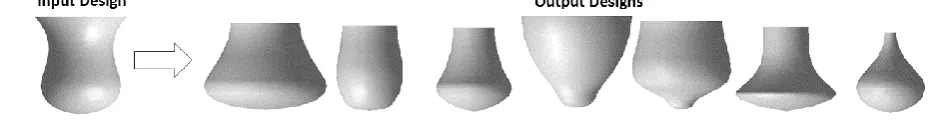
and infeasible designs in the dimension interval. In order to select a feasible one, enumeration is performed during the trails. All the candidate designs are enumerated in each trial and the one which minimizes the cost is selected. The cost function is defined based on the equality and inequality design constraints. A similarity constraint is applied based on the Euclidian distance formulation which ensures the generation of designs with variant geometries. Figure 1 shows designs generated using proposed methodology. A vasemodel is given as input and different designs are obtained. We believe that such automatic generation of CAD models can be very useful for design engineers and inspire them in the design process.

Figure 1. Variant shapes of vase model obtained by the proposed methodology

2. RELATED WORKS

Several improvements have been done by different researcher in order to improve LHS sampling. The method to perform uniform sampling in multidimensional space for LHS was introduced by Johnson et al. [3]. In this method, designs to be sampled using LHS are obtained while maximizing the minimum distance between designs (maximin criterion). The algorithm starts with a random design in the design space and searches for the next design with maximum of the minimum (maximin) inter-design distance. The maximin criterion was also used by Morris and Mitchell [4]. They used a simulated annealing search algorithm to search design space for designs which offer a compromise between the entropy and maximin criterion. Deutsch et al. [5] improved the method of maximin criterion by using Cholesky decomposition of correlation matrix and compared the proposed algorithm with simple LHS and Monte Carlo simulation. The obtained results showed that samples produced by their algorithm have better uniformity in the design space.

An algorithm for the best space filling designs was proposed by the Cioppa and Lucas [6]. However, their algorithm is computationally expensive because it requires the long run times. A Sliced Latin Hypercube (SLH) technique was introduced by Qian [7]. Design space is further sub-divided small design spaces and then sampling is performed in the sub-divided design spaces. This sub-division improves the space filling property of original LHS. SLH was further improved by Cao and liu [8]. They proposed a method which optimizes the sub-divided design space in order to maintain uniformity. Prescott [9] performed complete or partial enumeration searches to investigate the space-filling properties of orthogonal-column Latin Hypercube designs with multiple number of runs. He used the maximincriterion in cases where there are several designs with similar properties.

There are several other approaches proposed for the optimal distribution of designs in design space. Sacks et. al. [10] introduced a method of minimization of the integrated mean square error (IMSE). Shewry and Wynn performed selection of designs based on the maximization of entropy. Bates et. al. [11, 12] used approach of minimization of potential energy of designs according to Audze and Eglais [13]. Rajabi et. al. [14] studied the impact of initial design feed to LHS. They compared the effect of design selections randomly from the stratums and the selection of designs from the mid-point of stratums. The results revealed that design selection based on mid-point is significantly better than those based on random selection.

demonstrated by Bingham et. al. [17]. There is considerable amount of research has been done on optimal selection of designs in the design space in order to improve the space-filling property of LHS. However, most works done by researchers are proposed for the unconstrained design spaces. The research problem becomes very complicated when selection of designs has to be performed in a constrained and high dimensional design space, as that of the current research. Mysakova et al. [18] and Mysakova and Leps [19] proposed a technique to perform sampling for constrained spaces. This technique is based on the triangulation of admissible space by Delaunay Triangulation method. To produce uniform sampling in the design space, a heuristic method based on the uniform finite element meshes was proposed. Although this technique has good space filling property but it is just applicable to only two dimensional constraint problems. Fuerle and Sienz [20] proposed a method based on LHS for design selections for constrained spaces. Desired number of designs to be sampled are defined first and these points are then randomly sampled using LHS in two dimensional space. The coordinates of samples that are in infeasible region are modified using the mutation operator that is used for the genetic algorithms. Fuerle and Sienz method has some draw backs such that it cannot be implemented for the high dimensional sampling problems more than 3D. Furthermore, it does not produce good results for the designs space where infeasible designs are spread irregularly.

However, ELHS has the ability to perform sampling in more than three-dimension design spaces. ELHS also ensures the selection of variant feasible designs from the design spaces in which the distribution of the infeasible designs is highly irregular.

3. RESEARCH PROBLEM

LHS is a stratified sampling technique in which random samples of design can be generated from a multidimensional design space. Suppose an 𝑗 − 𝑑𝑖𝑚𝑒𝑛𝑠𝑖𝑜𝑛𝑎𝑙 design space and we want to sample 𝑗 number of designs evenly throughout the design space. The design parameters forms a specific

geometricaldesign (or design) and are denoted by 𝑥1, 𝑥2, 𝑥3, … , 𝑥𝑗. Each design parameter defines a

dimension in the design space. The value of each design parameter ranges between its lower and upper bound [𝑥𝑛𝑙, 𝑥𝑛𝑢] where 𝑛 = 1,2,3, … , 𝑗, 𝑥𝑛𝑙 and 𝑥𝑛𝑢 are the lower and upper bounds of the 𝑛𝑡ℎ design

parameter, respectively. The range of each design parameter is partitioned into 𝑁 + 1 equally spaced number of intervals (levels) such that [𝑥𝑛𝑙 = 𝑥𝑛1, 𝑥𝑛2, 𝑥𝑛3, … . . , 𝑥𝑛𝑁, 𝑥𝑛𝑁+1= 𝑥𝑛𝑢], where 𝑁 is the sampling

scale. The 𝑁 + 1 number of partitions of each dimension divides the design space into 𝑁𝑗 _{number of}

sub-spaces (stratums). LHS samples the designs from the stratums of design space and creates a design array (𝑇) which contain the sampled designs (see Figure 2 (c)).

During the search process of LHS to generate design array 𝑇, 𝑡 is the number of trials that are performed on the basis of LH-rule and 𝑡 = 𝑁. The LH-rule states that in any trial one and only one design can be selected from each interval of the design space. In the other trials, designs cannot be selected from a stratum of interval which is contiguous to the previous selected stratum (as case in Figure 2 (a)). For example, there are two designs (mark in black) are selected in the first trial as seen in the upper image of Figure 2 (a) which violated the LH-rule. During the second trial, a design is selected from the stratum that is contiguous to the previously selected stratum during trial-1 (see the lower image of Figure 2 (a)). This also violated the LH-rule. The Figure 2 (b) shows the sampling in the two dimensional design space satisfying the LH-rule.

There are feasible and infeasible designs in the constrained design space. The feasible design is one which satisfy the all geometrical constraints 𝜑1, 𝜑2, 𝜑3, … , 𝜑𝑚 which define relationships between the

for the selection of feasible designs based on LHS and for higher dimensional design space with equality and inequality constraints.

Figure 2. Implementation of LHS in the two dimensional design space with the sampling scale 𝑁 = 5. The red circle in the design space represents the sampled design. (a) Sampling is done while violating the LH-rule. (b) Sampling is done while satisfying the LH-rule. (c) Design array generated from the LHS implemented in image (b).

4. METHODOLOGY

The developed method gets a feasible design and its design space as input. Recall that a design space is formed using design parameters, design constraints and lower/upper bounds of each design parameter. Depending on the number of design to be sampled, 𝑁 (sampling scale) is also given. ELHS starts sampling the designs by performing trials in the design space. During a trial, candidate positions for each design parameter are enumerated and the candidate position having minimum cost value and satisfying the LH-ruleis selected.

To obtain designs with distinct geometries, a similarity threshold 𝜇 is utilized. During each trial, at most a feasible design is obtained and its distance to other previously selected designs should be greater than 𝜇. By doing this, we can store designs distinct from the previously obtained ones. Euclidean distance is utilized to compute distance between two designs 𝑝 and 𝑞 and calculated as follows: 𝐷𝑝𝑞 =

√∑𝑗_𝑛=1||𝑥_𝑛𝑝− 𝑥_𝑛𝑞||2 . 𝑥𝑛𝑝 and 𝑥𝑛𝑞 represents scaled parameter values for the designs 𝑝 and 𝑞 in the 𝑗 −th

dimension of the design space. The scaled parameter values are obtained after normalizing the parameter values between 0 and 1. These scaled parameter values forms the scaled design space. If all distances between the newly selected design and other previously obtained designs are greater than 𝜇, then newly selected design is stored. Otherwise it is rejected.

ELHS Algorithm:

1: //Input: initial feasible design 𝑋𝑖𝑛𝑖𝑡𝑖𝑎𝑙_{: [𝑥1 … 𝑥𝑗], lower and upper bounds [𝑥}

𝑛𝑙, 𝑥𝑛𝑢] of each

design parameter

2: Set the first design as 𝑋1= 𝑋𝑖𝑛𝑖𝑡𝑖𝑎𝑙 3: for 𝑡 = 1 𝑡𝑜 𝑁 do

4: Set 𝑥1 equal to 𝑡

5: for 𝑛 = 2 𝑡𝑜 𝑗 do 6: for 𝑝 = 1 𝑡𝑜 𝑁 do

7: Set 𝑥𝑛= 𝑝

8: Calculate cost value for design 𝑋𝑡

9: if cost value = 0 and LH-rulesatisfied then

10: Preserve 𝑝 for 𝑥𝑛

11: else

12: Reject 𝑝

13: end else 14: end if 15: end for 16: end for

17: // ℎ is total number of stored designs 18: for 𝑘 = 1 𝑡𝑜 ℎ

19: Calculate distance 𝐷𝑡𝑞 between 𝑋𝑡 and the 𝑘𝑡ℎ stored design 𝑋𝑞

20: if 𝐷𝑡𝑞 > 𝜇 then

21: Insert 𝑋𝑡 into the design array 𝑇 22: else

23: Reject 𝑋𝑡

24: end else 25: end if 26: end for 27: end for

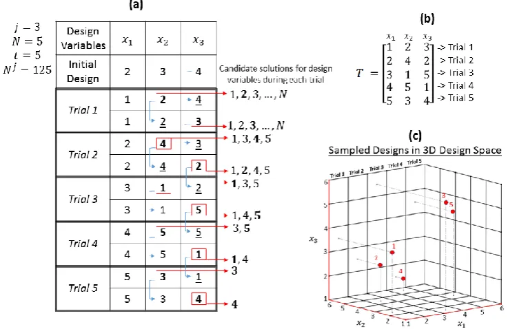
Here we illustrate the ELHS algorithm for a 3-dimensional design space. Therefore, design variables are denoted by 𝑥1, 𝑥2 and 𝑥3 representing each dimension of the design space (see Figure 3). Each

dimension is divided into 𝑁 + 1 divisions, where 𝑁 = 5. There are 125 stratums (𝑁𝑗= 125) and five trials will be performed (𝑡 = 5). Suppose the parameter set of initial input feasible design is

𝑋𝑖𝑛𝑖𝑡𝑖𝑎𝑙_{[2 3 4]. During the sampling process, positions of the first design variable are fixed from 1}

to 5 in order to decrease the total number of enumerations (see Figure 3 (a)). Using the input parameter set in the first trial 𝑥2 is enumerated for its available candidate positions 1, 2, … , 𝑁. During this

enumeration, position of 𝑥1 is set equal to 1 and position of 𝑥3 to 4 which is selected from input

parameter set. On the basis of cost function, 𝑥2= 2 is selected (see Figure 3 (a)). Proceeding to 𝑥3,

number of available candidate positions for the design parameter 𝑥3 are 1, 2, … , 𝑁. Enumeration is

performed for 𝑥3 between its candidate positions while taking 𝑥1 = 1 and 𝑥2= 2. During this

Figure 3. (a) Selection of candidate position during the trials. In which candidate position which minimizes the cost function is selected. (b) Design array containing the design. (c) 3-D plot of sampled designs.

In the second trial, 𝑥1 is set to 2 and enumeration is performed for 𝑥2 between its candidate positions

1, 3, 4, 5. According to LH-rule, as2 is already selected for 𝑥2 in the first trial, it cannot be selected in

the current trial. Therefore, 2 is eliminated from the candidate positions of 𝑥2 in second trial to validate

the LH-rule. In this trial, the candidate positions for 𝑥3 are 1, 2, 4, 5. The position 3 is eliminated to

validate the LH-rule, as it is selected in the first trial. Accordingly, the selection is done for the next three trials. Notice that in Figure 3 (a), number of candidate positions for design variables decreases as the number of trial increases because of the LH-rule. In the proposed technique, sampling process starts by taking 𝑋𝑖𝑛𝑡𝑖𝑎𝑙(input design) into account. As the proposed method is highly dependent on the input design, different inputs will apparently produce different designs.

4.1. Cost Function

Selection of designs during enumeration is done based on the cost function 𝐶𝑓 consisting of both equality

and inequality design constraints. During each trial, cost value is computed for all the candidate positions of a design parameter. The one which minimizes the cost function is selected. The cost function is formulated as follows:

𝐶𝑓= ∑ 𝐺(𝜑𝑚)

𝑙

𝑚=1

(1)

𝜑𝑚 represents a design constraint and 𝐺(𝜑𝑚) is the penalty function to penalize the design parameter

value that does not satisfy the constraint. Let 𝐹(𝜑𝑚) represents the equation of the design constraint 𝜑𝑚

which can be either 0 or greater/smaller then 0 for equality or inequality constraints, respectively. 𝐺(𝜑𝑚)

gets 0 if the equality or inequality constraint is satisfied. Otherwise, it is absolute value of 𝐹(𝜑𝑚) (see

Equation 2). With such formulation, 𝐶𝑓 is 0 for feasible designs and positive for infeasible ones.

𝐺(𝜑𝑚) = 0 𝑖𝑓 𝜑𝑚 𝑠𝑎𝑡𝑖𝑠𝑓𝑖𝑒𝑑

𝐺(𝜑𝑚) = |𝐹(𝜑𝑚)| 𝑖𝑓 𝜑𝑚 𝑛𝑜𝑡 𝑠𝑎𝑡𝑖𝑠𝑓𝑖𝑒𝑑

4.2. Multiple Run of the ELHS Algorithm

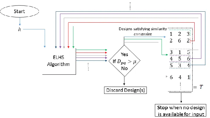
The ELHS algorithm is executed multiple times to increase the number of designs obtained. Number of designs obtained may not be equal to number of divisions 𝑁 after applying the ELHS algorithm. The algorithm runs multiple times until no design with distinct geometries are produced. The proposed method is dependent on the input design as previously stated. Different designs can be obtained by feeding different input designs to the ELHS algorithm.

Figure 4 illustrates the usage scenario of the ELHS algorithm. In the first run, the input design is the initial feasible design (𝑋𝑖𝑛𝑡𝑖𝑎𝑙) provided by the designer. The output of the first run is two variant feasible designs. In the second run, input to the ELHS algorithm-1 is the first design obtained from the first run.In third run, input is the second design obtained during the first run. Accordingly, multiple runs are performed until no distinct input design is obtained. Recall that distinctness is computed based on the similarity threshold 𝜇 in Section 4.

5. EXPERIMENTAL STUDIES

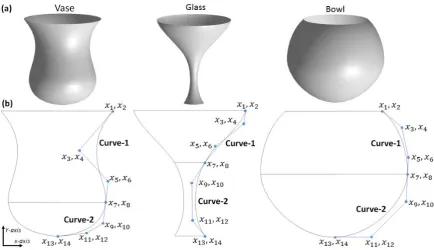
Several experiments have been conducted to check the efficiency of the proposed technique. Three different CAD models are selected as test models as seen Figure 5: Vase, glass and bowl.

Figure 5. Selected input CAD models to the proposed technique. (a) Surface models. (b) 2D wireframe models

5.1. Design Parameters

Number of design parameters and design constraints are kept same for the all three designs in order to verify and to gain better perspective of the behavior of the proposed method under the same design space. Each input design is composed of two cubic Bezier curves in X-Y plane and consists of fourteen design parameters (see Figure 5(b)). 3-D surfaces for these models are created by performing the revolve operation on the cubic Bezier curves around Y-axis. For better visual appearance, 𝐺0 _{and 𝐺}1 _continuity

is maintained at the connection of curve-1 and curve-2 of all three input designs. Design parameters (𝑥1, 𝑥2, 𝑥3, … , 𝑥14) are defined on the control points of curves as shown in Figure 5 (b). The design

parameters with odd integer numbered subscript represents the X-coordinate and design parameters with even integer numbered subscript represents the Y-coordinate of control points. For example, 𝑥1 and 𝑥2

are the X and Y-coordinate of the control point (𝑥1, 𝑥2), respectively.

5.2. Design Constraints

Seven design constraints are defined in Table 1 for the input CAD models that represents relationship between design parameters. 𝜑1, 𝜑2, … , 𝜑6 are the inequality constraints and 𝜑7 is the equality constraint.

𝜑7 is a nonlinear and maintains the 𝐺1 continuity between the curves at their connection point. 𝑣⃑1 is the

vector between control points (𝑥5, 𝑥6) and (𝑥7, 𝑥8), and 𝑣⃑2 is the vector between control points (𝑥7, 𝑥8)

and (𝑥9, 𝑥10). 𝜃 is the angle in radian between vector 𝑣⃑1 and 𝑣⃑2. If 𝜃 is zero, the connecting polygon

Table 1. Design constraints for the input CAD models

Design Constraints

𝜑1= 𝑥2− 𝑥4> 0 𝜑4= 𝑥8− 𝑥10> 0

𝜑2= 𝑥4− 𝑥6> 0 𝜑5= 𝑥10− 𝑥12> 0

𝜑3= 𝑥6− 𝑥8> 0 𝜑6= 𝑥12− 𝑥14> 0

𝜑7= 𝜃(𝑣⃑1, 𝑣⃑2) = 0

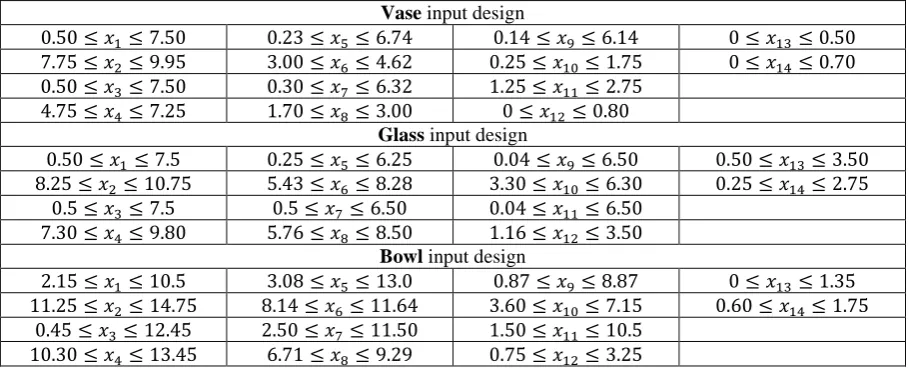
Table 2. Lower and upper bounds of design parameters of input CAD models

Vase input design

0.50 ≤ 𝑥1≤ 7.50 0.23 ≤ 𝑥5≤ 6.74 0.14 ≤ 𝑥9≤ 6.14 0 ≤ 𝑥13≤ 0.50

7.75 ≤ 𝑥2≤ 9.95 3.00 ≤ 𝑥6≤ 4.62 0.25 ≤ 𝑥10≤ 1.75 0 ≤ 𝑥14≤ 0.70

0.50 ≤ 𝑥3≤ 7.50 0.30 ≤ 𝑥7≤ 6.32 1.25 ≤ 𝑥11≤ 2.75

4.75 ≤ 𝑥4≤ 7.25 1.70 ≤ 𝑥8≤ 3.00 0 ≤ 𝑥12≤ 0.80

Glass input design

0.50 ≤ 𝑥1≤ 7.5 0.25 ≤ 𝑥5≤ 6.25 0.04 ≤ 𝑥9≤ 6.50 0.50 ≤ 𝑥13≤ 3.50

8.25 ≤ 𝑥2≤ 10.75 5.43 ≤ 𝑥6≤ 8.28 3.30 ≤ 𝑥10≤ 6.30 0.25 ≤ 𝑥14≤ 2.75

0.5 ≤ 𝑥3≤ 7.5 0.5 ≤ 𝑥7≤ 6.50 0.04 ≤ 𝑥11≤ 6.50

7.30 ≤ 𝑥4≤ 9.80 5.76 ≤ 𝑥8≤ 8.50 1.16 ≤ 𝑥12≤ 3.50

Bowl input design

2.15 ≤ 𝑥1≤ 10.5 3.08 ≤ 𝑥5≤ 13.0 0.87 ≤ 𝑥9≤ 8.87 0 ≤ 𝑥13≤ 1.35

11.25 ≤ 𝑥2≤ 14.75 8.14 ≤ 𝑥6≤ 11.64 3.60 ≤ 𝑥10≤ 7.15 0.60 ≤ 𝑥14≤ 1.75

0.45 ≤ 𝑥3≤ 12.45 2.50 ≤ 𝑥7≤ 11.50 1.50 ≤ 𝑥11≤ 10.5

10.30 ≤ 𝑥4≤ 13.45 6.71 ≤ 𝑥8≤ 9.29 0.75 ≤ 𝑥12≤ 3.25

6. RESULTS AND DISCUSSIONS

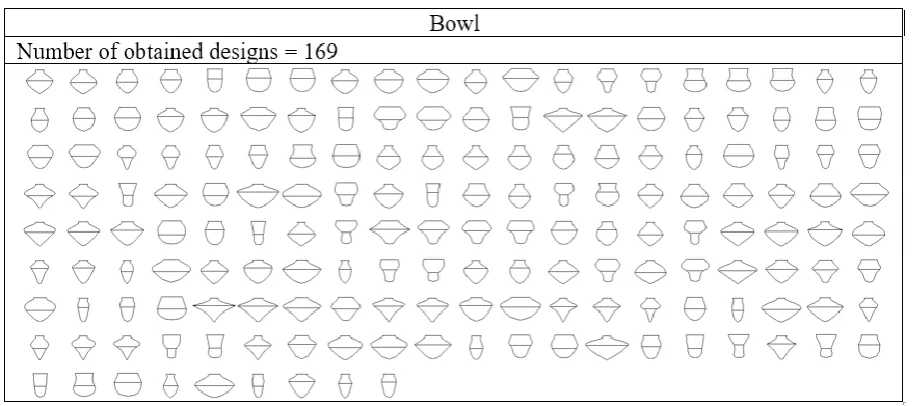
Figure 6 shows the test results obtained after inputting cup, glass and bowl models for 𝑁 = 200 and 𝜇 = 0.5 settings. The number of designs obtained after the single run of the ELHS algorithm are eight for the vase, 12 for the glass and seven for the bowl models. And the number of designs obtained by the multiple runs of ELHS algorithm are 223 for the vase, 293 for the glass and 169 for the bowl models. Naturally, greater number of designs are obtained for the multiple runs of the ELHS algorithm. The difference in the number of obtained designs for each input model is due to two factors. First, each input model has different design features, and secondly, the value ranges for the design parameters differs according to each input model. Notice that in Figure 6, distinct designs are obtained from both single run and multiple runs of the ELHS algorithm. The 𝐺0 _{and 𝐺}1 _{continuity is maintain at the connection}

points of curve-1 and curve-2 of the obtained designs.

Parameter Setting: Number of designs generated depends on the number of divisions of the design space. Figure 7 (a) shows the number of designs obtained for the vase model when using different values of 𝑁. Results here are obtained using the single run of the ELHS algorithm. For 𝑁 = 200, eight designs are obtained and 14 designs are obtained for the 𝑁 = 2000 setting. The maximum number of designs are obtained for 𝑁 = 1200 and remains constant for 𝑁 = 1700.

The similarity threshold 𝝁 is taken as 0.5 in the experiments that are shown in Figure 6. Note that diagonal of the scaled design space generated for the test models is √𝟏𝟒. With the increase in 𝝁, number of designs obtained decreases but distinction between these designs increases. Table 4 shows results for

𝝁 = 𝟎. 𝟓 and 𝝁 = 𝟏. 𝟎 settings when 𝑵 = 𝟐𝟎𝟎. For 𝝁 = 𝟎. 𝟓, 226 designs are obtained for the vase

Figure 6. Designs obtained by running the ELHS algorithm single and multiple times (𝑁 = 200 and 𝜇 = 0.5)

Figure 7. (a) Graph between number of designs obtained and number of design space divisions (𝑵) for vase model inputted to ELHS algorithm. (b) Graph between Computational Time and 𝑵 for vase model inputted to ELHS algorithm

Computational Time: A PC having the Intel Core i7 6700, 3.4 GHz processor and 16 GB memory is used for the experiments in this study. It is observed that computational time increases as the value of 𝑁 increases. Table 3 shows the processing time of the results provided in Figure 6. When 𝑁 is high, number of trials to be performed is also high and more number of candidate positions are available to enumerate in each trial. The computation for different values of 𝑁 for single run of the ELHS algorithm is shown in Figure 7 (b).

Table 3. Computational time of the results provided in Figure 6

Single run of ELHS Multiple runs of ELHS

𝑁 = 200 𝜇 = 0.5 𝑁 = 200 𝜇 = 0.5

Input Design Computational Time (sec) Computational Time (sec)

Vase 0.547 134

Glass 0.453 206

However, processing time decreases when 𝜇 is closer to 1 and increases when 𝜇 is closer to 0 for multiple runs of the ELHS algorithm. This is because of the fact that total number of runsdepends on the size of the design array. When value of 𝜇 is high, less designs are obtained in each run. And less number of runs are performed which results in less processing time. Table 4 shows computational times for 𝜇 = 0.5 and 𝜇 = 1.0 when vase model is inputted to ELHS algorithm. Multiple runs of the algorithm are done. In table 4, processing time is 0.585 minutes and number of obtained designs are 226 for the 𝑁 = 100 and 𝜇 = 0.5 settings. It means there are 266 number of runs are performed. On the other hand, processing time is 0.00571 minutes for 𝑁 = 100 and 𝜇 = 1.0 because only two algorithm runs are performed.

Table 4: Computational time and number of obtained designs for𝜇 = 0.5and𝜇 = 1.0

𝜇 = 0.5 𝜇 = 1.0

𝑁 Conputational Time (minutes)

Number of designs obtained

Conputational Time (minutes)

Number of designs obtained

100 0.585 226 0.00571 2

200 2.2 235 0.07 7

300 5.541 257 0.23 12

400 10.23 276 0.321 11

500 15.34 272 0.46 10

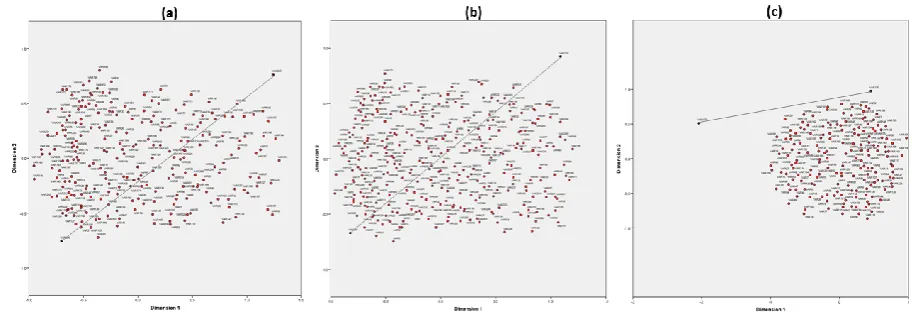
Distribution of obtained designs in the Scaled Design Space: In order to verify similarity between obtained designs Multidimensional scaling (MDS) is used [21]. The parameter values of designs in the design array (𝑇) are scaled between 0 to 1, and plotted on the 2-dimensional graph as shown in Figure 8. The red points in the graphs represents designs and line between two black points indicates the diagonal of the scaled space. The closeness of two point indicated their geometrical similarity. In Figure 8, image (a) and (b) and has better distributions of designs than image (c). Image (c) shows that in case of the bowl as input model, designs are not selected from the entire design space. This can occur because of different reasons, mainly: the empty region could be an infeasible region in the design space or the designs in this region may not satisfy the similarity constraints and get eliminated.

Limitation: A sampling technique is considered to have good space filling property, if the sampled designs are uniformly distributed throughout the design space. The designs obtained by ELHS does not guarantee the space filling property as it depends on the input design. However, the objective of current research to provide designers with a variety of design options for their product within the product’s design space is achieved.

7. CONCLUSIONS AND FUTURE WORKS

Latin Hypercube Sampling technique is extended in order to perform sampling in the high dimensional constrained design space with equality and inequality constraints. Designs space is formed by the designs parameters, designs constraints and lower/upper bounds for each design parameter. Each dimension of design space is divided into certain number of intervals to start the sampling process. The LH-rule is considered during sampling. ELHS starts the sampling process by performing enumeration during the trials. In every trial, all the candidate positons of each design parameter are enumerated and the one which minimizes the cost is selected. Designs with similar geometries are eliminated on the basis of similarity constraint and design with variant geometries are obtained.

As a future work, authors of current research will try to further improve the space filling property of the ELHS algorithm. Methods for the iterative improvements [22] will be studied and implemented in order to polish the sampling quality. Enumeration based operators can also be proposed for better uniformity of sampled designs. Other sampling techniques such as centroidal Voronoi tessellation and Latinization [23] will also be studied in order to check if these techniques can provide improved results.

ACKNOWLEGMENT

The authors would like to pay their deepest gratitude to the Scientific and Technological Research Council of Turkey (TÜBİTAK) for sponsoring this project (Project Number: 214M333).

REFERENCES

[1] MaKa M, Beckman R and Conover W. A comparision of three methods for selecting values of input variables in the analysis of output from computer code. Technimeterics 1979; 42: 55-61.

[2] Iman R, Conover W. Small sample sensitivity analysis techniques for computers models, with an application to risk assessment. Communications in statistics-theory and methods 1980; 9: 1749-1842.

[3] Johson R, Wichern D. Applied Multivariate Statistical Analysis. New Jersey. Prentice-Hall, 2002. pp. 767.

[4] Morris M, Mitchell T. Exploratory designs for computational experiments. Journal of Statistical Planning and Inference 1995; 43: 381-402.

[5] Deutsch J, Deutsch C. Latin hypercube sampling with multidimensional uniformity. Journal of Statistical Planning and Inference 2012; 142: 763-772.

[6] Cioppa T, Lucas T. Efficient nearly orthogonal and space-filling latin hypercubes. Technometrics 2007; 49: 45-55.

[8] Cao RY, Liu MQ. Construction of second-order orthogonal sliced Latin hypercube designs. Journal of Complexity 2014; 30: 762-772.

[9] Prescott P. Orthogonal-column Latin hypercube designs with small samples. Computational Statistics and Data Analysis 2009; 53: 1191-1200.

[10] Sacks J, Schiller S, Welch W. Designs for computer experiments. Technometrics 1989; 31: 41-47.

[11] Bates S, Sienz J, Langley D. Formulation of the Audze–Eglais uniform Latin hypercube design of experiments. Advances in Engineering Software 2003; 34: 493-506.

[12] Bates S, Sienz J, Toropov V. Formulation of the optimal latin hypercube design. In: 45th AIAA/ASME/ASCE/AHS/ASC Structures, Structural Dynamics & Materials Conference; 19-22 April 2004; Palm Springs, California.

[13] Audze P, Eglais V. New approach for planning out of experiments. Problems Dynam Strengths 1977; 35: 104-107.

[14] Rajabi M, Ashtiani B and Janssen H. Efficiency enhancement of optimized Latin hypercube sampling strategies: Application to Monte Carlo uncertainty analysis and meta-modeling. Advances in Water Resources 2015; 76: 127-139.

[15] Leary S, Bhaskar A, Keane A. Optimal orthogonal-array-based latin hypercubes. Journal of Applied Statistics 2003; 30: 585-598.

[16] Joseph V, Hung Y. Orthogonal-maximin latin hypercube designs. Statistica Sinica 2008; 18: 171-186.

[17] D. Bingham, R. Sitter, B. Tang. Orthogonal and nearly orthogonal designs for computer experiments. Biometrika 2009; 96: 51-65.

[18] Myšáková E, Lepš M, Kučerová A. A Method for Maximin Constrained Design of Experiments. In: Eighth International Conference on Engineering Computational Technology; 2012: Stirlingshire, Scotland.

[19] Mysakova E, Leps M. Method for Constrained Designs of Experiments in Two Dimensions. in: 18th International Conferance in Enginnering Mechanics; 14-17 May 2012; Svratka, Czech Republic. pp. 901-914.

[20] Fuerle F, Sienz J. Formulation of the Audze–Eglais uniform Latin hypercube design of experiments for constrained design spaces. Advances in Engineering Software 2011; 42: 680-689.

[21] Davison ML. Multidimensional scaling. Krieger Publishing Company.

[22] Liefvendahl M, Stocki R. A study on algorithms for optimization of Latin Hypercubes. Journal of Statistical Planning and inference 2006; 136: 3231-3247.