Solving Hard Graph Problems with Combinatorial Computing and Optimization

(1)

Theses

Thesis/Dissertation Collections

6-2013

Solving Hard Graph Problems with Combinatorial

Computing and Optimization

Alexander R. Lange

Follow this and additional works at:

http://scholarworks.rit.edu/theses

This Thesis is brought to you for free and open access by the Thesis/Dissertation Collections at RIT Scholar Works. It has been accepted for inclusion in Theses by an authorized administrator of RIT Scholar Works. For more information, please [email protected].

Recommended Citation

(2)

Combinatorial Computing and

Optimization

by

Alexander R. Lange

A Thesis Submitted in

Partial Fulfillment of the Requirements for the Degree of

Master of Science in

Computer Science

Supervised by

Dr. Stanis law Radziszowski

Department of Computer Science

B. Thomas Golisano College of Computing and Information Sciences Rochester Institute of Technology

Rochester, New York

(3)

The thesis “Solving Hard Graph Problems with Combinatorial Computing and

Optimiza-tion” by Alexander R. Lange has been examined and approved by the following Examination

Committee:

Dr. Stanis law Radziszowski Professor

Thesis Committee Chair

Dr. Ivona Bez´akov´a Associate Professor Reader

Dr. Darren A. Narayan Professor

(4)

Dedication

This thesis is dedicated to Blair Phillips, a truly remarkable and special human being whom

I was fortunate enough to call my good friend for the better part of my life. I have looked up

to you since I was eight years old, and I know I speak for an uncountable number of people

when I say there are an uncountable number of ways I am thankful to have known you.

I recall the look on your face from the night I eagerly explained to you this cool math I

just learned called Ramsey theory. It was a look of curiosity, of admiration, of excitement; a

look that was as native to you as your red hair. I am thankful that you were there when all

(5)

Acknowledgments

I am fortunate to owe many people many thanks for who and where I am today.

First, I thank my family and friends for their constant stream of support. I give special

thanks to my parents for always being there, for pushing me, and for instilling in me my

enjoyment of learning. I thank my brother, Jake, for reminding me to still have fun. I also

thank: the Avon group for the enduring foundation; Eli and Matt for assuring my academic

interests; Pete for the emergency IT support; Tori for saying it was “really cool” the first

night I was too busy with work; Harwin and BTZ for the nights of needed distraction; and

Izzy for hanging out on the many nights of no distraction.

The Mathematics and Computer Science faculty and staff have been great to me. I thank

Professor Narayan for being on my thesis committee, and for welcoming me into the REU

these past two summers. I thank Ivona for reading my thesis, and especially thank her and

Edith for the numerous opportunities I have been given to appreciate, explore, and build

my confidence in many areas of computer science theory.

I did not accomplish this work on my own. I thank Ivan Livinsky and Xiaodong Xu for

collaborating with me, as well as Yongqi Sun and my many peers at RIT. I owe many thanks

to Gurcharan Khanna and Research Computing at RIT for the valuable and helpful support,

as well as Mats Rynge for his guidance throughout my use of the Open Science Grid.

Last and far from least I thank Staszek for his mentorship, including his distinctive and

persistent confidence, patience, and integrity. I am forever indebted to him not only for the

many opportunities he has presented me, but for introducing me to a world of mathematics

(6)

Chapter 1

Introduction

1.1

Overview

This thesis is concerned with problems arising in graph theory, and how the use of

computa-tions can assist in determining their solucomputa-tions. The problems of interest are those which

are difficult by nature, and are often associated with problems known to be NP-complete.

It is therefore unlikely to be able to develop efficient, exact algorithms to solve them, and

alternative computational methods are used instead. Combinatorial computing is a branch

of mathematics and computer science concerned with such methods, where algorithms

are invented and implemented to generate, enumerate and search through combinatorial

structures. In this thesis, we study and implement techniques for attacking instances of such

problems which are too large to solve “by hand.” Some success is obtained, as summarized

below.

A number of problems studied in this thesis fall under the branch of mathematics

known as Ramsey theory. This subject is primarily concerned with the properties certain

mathematical structures need in order to guarantee that desired sub-structures are contained

within them. It is often seen as the study of the order that can be derived from chaos.

Graphs are combinatorial objects that Ramsey theory is regularly associated with.

A classical problem used to introduce Ramsey theory involves a party in which some

people are mutual acquaintances and all others are mutual strangers. The problem asks

to determine the minimum number of people needed at such a party so that either three

people all know each other or three people all don’t know each other. It is straightforward

to represent this as a graph problem: Let each person be represented as a vertex and let all

vertices be connected to each other, that is, let the graph be complete. We will color each

(10)

is then to find the minimum n such that the complete graph Kn, when colored this way,

always contains either a red or blue triangle. This nis the Ramsey numberR(3,3) and it is

known that R(3,3) = 6.

In 1967, Erd˝os and Hajnal [40] posed the question: Does there exist a K4-free graph

that is not the disjoint union of two triangle-free graphs? This question is similar to the

previous, but instead of coloring the edges of the complete graph, we color those of a

K4-free graph. In 1970, Folkman [49] proved that they indeed exist, and they are now called

Folkman graphs. The problem then became to determine how small such a graph could

be, known as the Folkman number Fe(3,3; 4). The difficulty of this task is apparent, as

the best known bounds prior to this work were 19≤Fe(3,3; 4)≤941. In the first part of

this thesis, we employ computational techniques to improve the upper bound to 786. These

techniques combine known methods with a novel use of the Goemans-Williamson MAX-CUT

semidefinite programming relaxation, as described in Chapter 2.

Analogous Ramsey-type problems exist for graphs different than triangles. The Ramsey

number R(G, H) is the smallest nsuch that for every two-coloring of the edges of Kn, a

monochromatic copy of G or H exists in the first or second color, respectively. A main

combinatorial computing approach in determining R(G, H) is to computationally construct

colorings ofKtthat do not contain copies ofGin the first color or copies ofH in the second,

thus establishing R(G, H) > t. If a complete enumeration of such colorings is possible,

we can determine R(G, H) exactly. Chapter 3 is concerned with such an approach for

R(C4, Km), where C4 is the cycle on four vertices. With the use of massive computations

on the Open Science Grid, we determine R(C4, K9) = 30 and R(C4, K10) = 36.

A main goal of this thesis was to apply known techniques in lattice basis reduction to

new combinatorial problems, especially those associated with Ramsey theory. The

Lenstra-Lenstra-Lov´asz (LLL) algorithm is a well-known, polynomial-time algorithm that, when

given a basis of a lattice, returns a reduced basis for the same lattice containing the shortest

vectors it can find. Its main application to combinatorial computing involves representing a

search problem in a particular matrix form, so that if the column vectors of the matrix are

treated as a basis of a lattice, the solution to the problem is found as a short vector of a

reduced basis of that lattice.

(11)

some success in applying basis reduction to another area of graph theory: graph domination.

A classical problem associated with this area is one involving the game of chess. The question,

originally studied by de Jaenisch in 1862 [35], asks: What is the minimum number of queens

needed, so that if placed on an n×nchessboard, a piece on any other position is capturable

by a queen? This problem, like the party problem, can be formulated with a graph. Let

each position of a chessboard be a vertex and let two vertices be connected if a queen on

the first position can reach the second position in one move. The question is then to find

the smallest collection of vertices such that all other vertices are connected to at least one of

the collection. This is the problem of graph domination. Chapter 4 presents a method that

uses the LLL Algorithm to find dominating sets of a graph and presents experimental data

exhibiting some success.

As previously mentioned, the common thread of this work is the use of computations

in solving specific instances of graph problems which are believed to be too large to be

solved by hand. Before discussing the details of these computations in Section 1.3, we now

introduce the concepts and notation used throughout this work.

1.2

Background and Notation

Graph Theory

The main theme common to all parts of this thesis is that of graph theory. Agraph G is a

set of vertices andedges where edges are unordered pairs of vertices. V(G) andE(G) are

the vertex set and edge set of G, respectively. If{u, v} ∈E(G) thenu andvare adjacent or

connected vertices, and both u andv are incident to edge{u, v}. All graphs in this work

are loopless (for anyv∈V(G), {v, v} 6∈E(G)) and unweighted. Theorder of G is|V(G)|

and the size of Gis |E(G)|. The complement of G, denotedG, is defined asV(G) =V(G)

and E(G) ={{u, v} | {u, v} 6∈E(G) and u6=v}. A subgraph ofG is a graphH such that

V(H) ⊆ V(G) and E(H) ⊆ {{u, v}| u, v ∈ V(H), {u, v} ∈ E(G)}. A directed graph or

digraph is a graph in which the edge set is ordered, that is, (u, v) and (v, u) are distinct

edges. A bipartite graph is a graph whose vertices can be split into two parts such that no

two vertices in the same part are adjacent. Acirculant graph C on nvertices is defined as

(12)

The neighborhood of v ∈ V(G) is the set of vertices adjacent to v, and is denoted

NG(v) ={u| {u, v} ∈E(G)}. The closed neighborhood of v isNG[v] = NG(v)∪ {v}. The

degree of v is deg_G(v) =|NG(v)|. The minimum and maximum degrees of vertices inG are

denoted δ(G) and ∆(G), respectively. G is d-regular if deg_G(v) =d for allv ∈ V(G). A

subgraphH of Gis an induced subgraph ifE(H) ={{u, v}|u, v∈V(H), {u, v} ∈E(G)},

that is, H has all of the edges Ghas over V(H). If S=V(H), we say H is induced byS

and write H=G[S]. The join of two graphsG1+G2 =Gis the union of G1 and G2 with

every vertex of G1 connected to every vertex of G2, that is, V(G) =V(G1)∪V(G2) and

E(G) =E(G1)∪E(G2)∪ {{g1, g2} |g1∈V(G1), g2 ∈V(G2)}.

We use common notation to represent important types of graphs that appear throughout

this work: Kn is thecomplete graph onnvertices, where every pair of vertices is connected;

Ks,t is thecomplete bipartite graph, a bipartite graph with parts of order sandt, where each

vertex of one part is connected to all of the other;Cn is then-vertexcycle graph, consisting

of only a simple cycle; Pn is an n-vertexpath graph, consisting of only a simple path;Wn is

the wheel graph, defined as K1+Cn−1; and St is thestar graph, defined asK1,t.

We now introduce a number of classical graph properties whose related problems and

parameters are explored throughout this thesis. A clique of ordern is a subset ofn vertices

of a graph such that each vertex is adjacent to every other vertex. An independent set is the

complement of a clique. The maximum clique and maximum independent set of a graphGare

theclique number ω(G) and theindependence numberα(G), respectively. Acut is a partition

of the vertices of a graph into two sets, S ⊂V(G) andS=V(G)\S. The size of a cut is

the number of edges that join the two parts, that is, |{{u, v} ∈E(G)|u∈S and v ∈S}|.

MAX-CUT is a well-known combinatorial optimization problem that asks for the maximum

size of a cut of a graph, which we denote asM C(G). A set D⊆V(G) is adominating set

ofGif every vertex is either in Dor adjacent to a vertex inD. A vertexudominates vertex

v ifu=v or {u, v} ∈E(G). The minimum order of such a set is thedomination number

and is denotedγ(G).

An important concept of this thesis is that of the Ramsey arrowing operator. Given graphs

(G1, G2, . . . , Gk), we writeG→(G1, G2, . . . , Gk) and sayGarrows (G1, G2, . . . , Gk) if for any

k-coloring of the edges ofG, a monochromaticGi exists for some colori∈ {1, . . . , k}. When

(13)

[image:13.612.265.351.89.176.2]

Figure 1.1: Unique coloring ofK5showingK56→(3,3)

the smallest nsuch thatKn→(G1, G2, . . . , Gk). TheFolkman number Fe(s1, s2, . . . , sk;k)

is the order of the smallest Kk-free graph that arrows (s1, s2, . . . , sk).

We know that Ramsey numbers exist due to the seminal paper by Frank P. Ramsey in

1930 [125]. As previously mentioned, a classical small example isR(3,3) = 6. Note that this

means that K56→(3,3) andK6→(3,3). The unique witness of K56→(3,3) is presented in

Figure 1.1, where each of the two colors is isomorphic to C5. Proving K6 → (3,3) was a

problem of the 1953William Lowell Putnam Mathematical Competition. Consider a red-blue

edge coloring of K6. Asv∈V(G) is incident to 5 edges, at least three of them will be the

same color, say red without loss of generality. The three other vertices incident to these

red edges are also connected. None of these connections can be red, or else a red triangle

is formed with v. However, if they are all colored blue, they form a blue triangle. Thus,

K6 →(3,3).

In general, research involving Ramsey numbers is split into two areas. In one, the

question is how the numbers behave asymptotically, that is, how for exampleR(3, k) behaves

as k approaches infinity. The other is concerned with determining values and bounds for

numbers with small parameters. A main goal of the latter is to provide insight that quantifies

results of the former. In Chapter 3, we present what is known about the asymptotics of

R(C4, Km), and focus our work on computational attacks on the small numbers.

We approach these and related graph parameters and problems with a computational

perspective. Determining ω(G),α(G),M C(G), orγ(G) for a general graph GisNP-hard,

and the corresponding decision problems are NP-complete (see [54]). Many Ramsey graph

coloring problems are NP-hard or lie even higher in the polynomial hierarchy; we discuss

some such problems in Section 2.2. It is straightforward to see that deciding Ramsey arrowing

(14)

these properties is a main motivation for studying how computational techniques within

combinatorics and optimization can aid in solving specific instances of them.

Linear Algebra

Through out this work, a variable in boldface represents a vector in eitherRn orZn, the

vector spaces of all n-dimensional vectors with real or integer entries, respectively. The

entries of vectorvare denotedv1, v2, . . . , vn. Unless otherwise specified,kvkis the Euclidean

norm of v∈_Rn_{, defined as}

kvk=

q

v₁2+v2₂+· · ·+v2

n.

We use0and1to denote vectors whose entries consist of all 0’s or 1’s, respectively. Matrices

are represented with capital letters, such as, for example, A for the adjacency matrix of a

graph, orV for a matrix with column vectorsv1,v2, . . . ,vk.

Given a set of linear independent vectorsB ={b1,b2, . . . ,bn}, the span of B is the set

of all linear combinations of them. Let span(B) =S; S is asubspace ofRn andB is a basis

of S. If the linear combinations ofB are restricted to those with integer coefficients, that is,

span_Z(B) =

( _n

X

i=1

xibi|xi∈Z, for 1≤i≤n

)

,

then L= span_Z(B) is the lattice with basisB. Lattices are discussed in detail in Chapter 4.

Mathematical Programming

A linear program (LP) asks to find the optimal value of a linear function subject to linear

equality and inequality constraints (see for example [140, 126]). The standard form of a

linear program is the maximization of the function f(x), x∈Rn_{, formulated as:}

Maximize f(x) = n

X

i=1

cixi (1.1)

subject to: n

X

i=1

aijxi ≤bj, j = 1,2, . . . , m,

(15)

Note that (1.1) can be rewritten in matrix form as

max{cTx|Ax≤b and x≥0},

and that the minimization of f(x) can be determined by the maximization of−f(x).

Linear programming has many applications in a wide variety of areas, including

busi-ness, economics, engineering, and operations research, and was first developed by Leonid

Kantorovich in 1939 for use in World War II (see [80]). Many efficient algorithms exist for

solving LPs, including the well-known simplex and interior point methods, the latter of

which run in polynomial time. The efficiency of these algorithms relies on the geometry

of the constraints (see [65, 143]). A set S ⊂_Rn _is _convex _{if and only if the line segment}

connecting any two u,v∈S, defined as {αu+ (1−α)v|0≤α≤1}, is contained in S. If

the constraints of an LP are viewed as a hyperplane in Rn, then the intersection of their

feasible regions forms a polytope, ann-dimensional geometric object with “flat” sides. The

solution of the LP will lie on one of the points of this polytope, all of which form a convex

set. The simplex method, for example, uses this geometry to “walk” from point to point

until the optimal one is found.

Aninteger program (IP) is a mathematical optimization program that restricts some

or all of its variables to integers. An integer linear program (ILP) is an LP with the

additional restriction that x∈_Zn_{. Unlike linear programming, integer programming tends}

to be computationally difficult; ILP is known to be NP-hard. The additional restriction

of x ∈ {0,1}n _{is one of Karp’s 21} _NP_{-complete problems [83]. Although this implies}

that the existence of a polynomial-time algorithm for solving IPs is unlikely, the fact that

many combinatorial optimization problems can be formulated as them has resulted the area

becoming an extensive subject. Many techniques are known to perform well for certain

problems (see e.g. [112, 81]). A main thrust of this thesis involves formulating the previously

described hard graph problems as integer programs, and then using some heuristic or

bounding technique to find or approximate a solution.

Asemidefinite program(SDP) is a linear program where the solution vectorxis replaced

with a positive semidefinite matrix [55]. A matrixX ispositive semidefinite, denoted X0,

(16)

Maximize n

X

i,j

cijxij (1.2)

subject to: n

X

i,j

aijkxij =bk, k= 1,2, . . . , m,

X0.

SDPs are convex optimization problems and, similarly to linear programs, can be solved

with efficient algorithms, such as interior point methods.

1.3

Computational Thrust

A substantial part of this thesis involved the development of software to generate and

manipulate graphs for use in experiments. The base of our software includes a library

containing a robust graph data structure; it was used in all three parts of this work. Vertices

and their associated adjacency lists are represented as bitsets with basic set operations

accomplished using bitwise operations, as described in [93]. Our library includes over 80

functions that perform tasks ranging from simple (such as adding edges and determining the

minimum degree) to complex (such as computing MAX-CLIQUE with pruned backtracking).

We also implemented functionality to generate a large variety of graphs, including random

graphs, Paley graphs, and graphs joined from multiple smaller graphs. Such graphs are

explained in more detail in Section 2.4.2. A notable tool we developed for the Fe(3,3; 4)

research is archer, an interactive prompt that calls the library to create, manipulate, and

output graphs in real-time.

The computational attack onR(C4, Km) required us to implement a number of additional

combinatorial algorithms optimized to be as fast and as cheap as possible. We routinely tested

the software, and often modified the code multiple times a week during the experimentation

phase. The software’s success was partly due to our consideration of aspects often overlooked,

such as minimizing the size of the data types we used. The computations were made possible

due to the Open Science Grid (OSG), a multidisciplinary initiative joining the resources

of various cyberinfrastructures to meet the needs of academic computing of all sizes. We

(17)

algorithms and use of the OSG is discussed in detail in Section 3.5.

LLL and related basis reduction algorithms were implemented with the use of FLENS

[66], a C++ library that is essentially an intuitive wrapper for the established linear algebra

libraries BLAS and LAPACK. We implemented the algorithms this way in order to make

use of the graph libraries previously described. Additional functions were written to convert

graph problems to search problems involving vectors of lattice bases. This is described in

more detail in Section 4.4.6.

All code was written in C++ and most tests were performed on Linux systems. Various

bash scripts were written for batch experiments. All source code can be found in public

githubrepositories [97].

In addition to our own code, we made use of a number of third-party software packages.

Graph isomorphism testing, an essential part of graph enumeration, was performed using

Brendan McKay’s well-known nauty software [109]. In some cases, our code was compiled

directly with nautylibraries, while in others the standalone tools of the software were used.

The work discussed in Chapter 2 makes use of a number of extra software, including MATLAB

[108], SDP solvers [14, 72], and SAT solvers [56, 5]. The Number Theory Library by Victor

Shoup [133] was called when operations under Galois fields were needed. Finally,sage [137],

an open source mathematical software built on Python, was used for verification of properties

of our data, special graph generation, and the analysis of some graph automorphism groups.

1.4

Structure of Thesis

The structure of this thesis is as follows:

Chapter 2 discusses edge Folkman problems concerning triangles. Specific focus is placed

on the Folkman numberFe(3,3; 4), which asks for the smallest order of aK4-free graph that

is not the union of two triangle-free graphs. The main result of this work is an improvement

of the upper bound to Fe(3,3; 4)≤786. A significant aspect of this result is the use of the

Goemans-Williamson MAX-CUT SDP relaxation.

Chapter 3 studies the Ramsey numbers R(C4, Km), which is the smallestn such that

every graph on nvertices contains either a C4 or independent set of order m. We present

(18)

We conclude the chapter with a discussion on the computational approach to attacking these

numbers, and establishR(C4, K9) = 30 and R(C4, K10) = 36 with large grid computations

on the Open Science Grid.

Chapter 4 includes an overview of the Lenstra-Lenstra-Lov´asz (LLL) algorithm, a

well-known, polynomial-time algorithm that, when given a basis of a lattice, returns a reduced

basis for the same lattice with the shortest vectors it can find. We include a summary

of lattices and basis reduction techniques, the algorithm’s applications to combinatorial

computing, and present a method which makes use of it as a heuristic for computing a

graph’s domination number.

We present a number of theorems throughout this thesis. Those that do not contain

citations are our original work, while those that include citations are previously known

results. In some cases we provide proofs for the theorems which are not our own. This is

mostly done to provide insight into our work, but sometimes proofs are presented simply

(19)

Chapter 2

Folkman Number

F

e

(3

,

3; 4)

2.1

Introduction

Given a graph G, we write G→(a1, . . . , ak) and say thatGarrows (a1, . . . , ak) if for every

edge k-coloring of G, a monochromatic Kai is forced for some colori∈ {1, . . . , k}. Likewise,

for graphs F andH, G→(F, H) if for every edge 2-coloring ofG, a monochromatic F is

forced in the first color or a monochromaticHis forced in the second. DefineF_e(a1, . . . , ak;p)

to be the set of all graphs that arrow (a1, . . . , ak) and do not contain Kp; they are often

called Folkman graphs. The edge Folkman number Fe(a1, . . . , ak;p) is the smallest order

of a graph that is a member of Fe(a1, . . . , ak;p). In 1970, Folkman [49] showed that for

k >max{s, t},Fe(s, t;k) exists. The related problem of vertex Folkman numbersFv(s, t;k),

where vertices are colored instead of edges, is more studied (see e.g [106, 114]) than edge

Folkman numbers, but we will not be discussing them in detail.

In 1967, Erd˝os and Hajnal [40] asked the question: Does there exist aK4-free graph that

is not the union of two triangle-free graphs? This question is equivalent to asking for the

existence of a K4-free graph such that in any edge 2-coloring, a monochromatic triangle is

forced. After Folkman proved the existence of such a graph, the question then became to find

how small this graph could be, or using the above notation, what is the value of Fe(3,3; 4).

Prior to this work, the best known bounds for this number were 19 ≤ Fe(3,3; 4) ≤ 941

[124, 36].

An improvement to the upper bound of the Folkman number Fe(s, t;k) requires one

Kk-free witness that arrows (s, t), while an improvement to the lower bound requires a proof

that all graphs of a given order have no such property. This is perhaps a reason for the

puzzling large range between the lower and upper bounds of Fe(3,3; 4). Clearly in this case,

(20)

2.1.1 Overview of Fe(3,3;k)

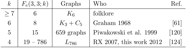
Table 2.1 summarizes known results forFe(3,3;k). Since the Ramsey number R(3,3) = 6, it

follows that Fe(3,3;k) = 6 fork≥7. In 1968, Graham [61] responded to Erd˝os and Hajnal

by presenting an explicit K6-free graph on 8 vertices that arrows (3,3). As no such graph

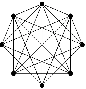
exists with 7 vertices, this showedFe(3,3; 6) = 8. This graph,K8−C5, is displayed in Figure

2.1, and a summary of the proof that K8−C5=K3+C5 →(3,3) is found in Theorem 1.

k Fe(3,3;k) Graphs Who Ref.

≥7 6 K6 folklore

6 8 K3+C5 Graham 1968 [61]

5 15 659 graphs Piwakowski et al. 1999 [120]

[image:20.612.148.472.223.305.2]

4 19 – 786 L786 RX 2007, this work 2012 [124]

Table 2.1: Known values and bounds forFe(3,3;k)

Theorem 1 (Graham, 1968 [61]). G=K8−C5 =K3+C5→(3,3)

Proof. Assume there is an edge coloring of G such that neither of the colors contain a

triangle; call the parts of this coloring R (red) and B (blue). Consider the triangle of G

that is joined to C5. Two of the vertices in this triangle will be incident to a red and blue

edge, as the K3 is non-monochromatic. Let one of those vertices bev. This vertex will be

adjacent to all five vertices c1, . . . , c5 of theC5. At least 3 of these edges will be one color,

so without loss of generality, say {v, c1},{v, c2},{v, c3} ∈ B. Two of {c1, c2, c3} must be

adjacent, say{c1, c2} ∈E(C5). Clearly,{c1, c2} must be red to avoid a blue triangle. Pick

u ∈V(K3) such that {u, v} ∈ B. Then, neither {u, c1} nor {u, c2} can be in B or a blue

triangle is formed. However, if they are both red, then they form a red triangle with{c1, c2}.

Therefore, a monochromatic triangle must exist.

The case for k = 5 received much attention up until 1999, when Piwakowski et al.

determined that Fe(3,3; 5) = 15 [120]. The first upper boundFe(3,3; 5)≤42 was obtained

by Sch¨auble in 1969 [131], although the proof of existence is credited to an unpublished

work by P´osa. In 1971, Graham and Spencer [62] improved the bound to Fe(3,3; 5)≤23.

Both constructions rely on cleverly connecting a number of C5 graphs and a triangle. The

(21)

[image:21.612.234.385.87.242.2]

Figure 2.1: K8−C5, the witness ofFe(3,3; 6) = 8

1979 [67], and 15 by Nenov in 1981 [113]. The latter two results were published in Russian

and seemed to go unnoticed for some time.

The computational approach by Piwakowski et al. to determine Fe(3,3; 5)≥15 involved

processing a large number of graphs to show that no 14-vertex graph exists in Fe(3,3; 5).

Since R(3,5) = 14, any 14-vertex graphG∈ F_e(3,3; 5) will contain aK3. They determined

a number of properties ofG\K3, and all graphs on 11 vertices with these properties were

processed in order to reconstruct graphs G. However, no such graphs were found.

Figure 2.2 presents the unique bicritical 15-vertex graph in Fe(3,3; 5). It is bicritical

because (a) adding any edge forms a K5 and (b) removing any edge makes it not arrow (3,3).

This graph plays an important role in the vertex Folkman number Fv(3,3; 4), as removing

vertex v yields the unique bicritical witness ofFv(3,3; 4) = 14.

The focus of this chapter is on the most studied open Folkman number,Fe(3,3; 4), and

ways the well-known graph MAX-CUT problem can determine arrowing of triangles. The

next section overviews the rich history of this number.

2.2

History of

F

e

(3

,

3; 4)

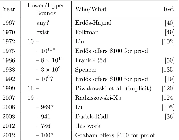
Table 2.2 summarizes the events surroundingFe(3,3; 4), starting with Erd˝os and Hajnal’s

[40] original question of existence. After Folkman [49] proved the existence, Erd˝os, in 1975,

offered $100 for deciding ifFe(3,3; 4)<1010.

(22)

[image:22.612.220.398.87.254.2]

v

Figure 2.2: Only bicritical graph of all 659 witnesses toFe(3,3; 5) = 15, wherev is

connected to all other 14 vertices.

by Goodman in 1959 [60], which involves counting the triangles of an edge-colored graph.

Note that there is essentially a single coloring of a non-monochromatic triangle: two edges

are one color and one edge is the other. A non-monochromatic triangle therefore has two

vertices that are incident to both a red and blue edge. Let G be an edge-colored graph

with no monochromatic triangles. LettRB(x) count the triangles {x, y, z} where{x, y} is

red and {x, z} is blue; then, P

v∈V(G)tRB(v) = 2t4(G). If Gx is the induced subgraph of

NG(x), then each edge in Gx counts a triangle, yielding

P

v∈V(G)|E(Gv)|= 3t4(G). Since no monochromatic triangle exists, the vertices of each Gx can be partitioned such that

M C(Gx) =tRB(x). Combining these equations gives

P

v∈V(G)M C(Gv) =23|E(Gv)|.

However, if every coloring of a graphGcontains a monochromatic triangle, then some

Gv can not be partitioned completely, resulting in Theorem 2.

Theorem 2 (Spencer, 1988 [135]). LetGbe a graph and Gv be the graph induced byNG(v).

If

X

v∈V(G)

M C(Gv)< 2

3|E(Gv)|,

then G→(3,3).

Deciding Fe(3,3; 4)<1010 remained open for over 10 years. Frankl and R¨odl [50] nearly

met Erd˝os’ request in 1986 when they showed thatFe(3,3; 4)<7.02×1011using probabilistic

arguments and ideas similar to those described above. In 1988, Spencer [135], in a seminal

(23)

Year Lower/Upper

Bounds Who/What Ref.

1967 any? Erd˝os-Hajnal [40]

1970 exist Folkman [49]

1972 10 – Lin [102]

1975 – 1010? Erd˝os offers $100 for proof

1986 – 8×1011 Frankl-R¨odl [50]

1988 – 3×109 Spencer [135] 1992 – 106? Erd˝os offers $100 for proof [19] 1999 16 – Piwakowski et al. (implicit) [120]

2007 19 – Radziszowski-Xu [124]

2008 – 9697 Lu [105]

2008 – 941 Dudek-R¨odl [36]

2012 – 786 this work

[image:23.612.154.465.89.332.2]

2012 – 100? Graham offers$100 for proof

Table 2.2: Timeline of progress onFe(3,3; 4).

graph of order 3×109 _{(after an erratum by Hovey) without explicitly constructing it. The}

main idea behind his result involved G=G(n, p), the random graph with n vertices and

edge probability p. From this graph, a K4-free graphG∗ is obtained by randomly removing

an edge from each K4 in G. By setting n = 3×109, he showed that a G∗ satisfying the

condition in Theorem 2 exists with positive probability.

Erd˝os then offered $100 for deciding if Fe(3,3; 4) < 106 (see [19], page 46). Much

time passed until 2007, when Lu and Dudek-R¨odl independently showed it to be true. Lu

determined Fe(3,3; 4)≤9697 by constructing a family ofK4-free circulant graphs (which we

discuss in Section 2.5) and showing that some such graphs arrow (3,3) using a combination

of spectral analysis and Theorem 2. The main idea behind his proof involves a graph H

being δ-fair if M C(H) < (1₂ +δ)|E(H)|. From Theorem 2 it follows that if each Hv is

1

6-fair, thenH→(3,3). Lu was able to show thatd-regular graphs wereδ-fair if the smallest

eigenvalue of the adjacency matrix was greater than−2δd, and found a number of “small”

graphs, including one with order 9697, that had this property.

Dudek and R¨odl reduced the upper bound to the best known to date, 941. Their method,

which we have pursued further with some success, is discussed in the next section. A natural

(24)

Mathematics in Halifax, Nova Scotia, Ronald Graham announced a $100 award for deciding

this. We discuss a possible witness for this bound in Section 2.4.1.

The lower bound for Fe(3,3; 4) has been much less studied than the upper bound. Lin

[102] obtained a lower bound on 10 in 1972. Without the help of a computer, he showed

that Fe(a1, . . . , ak;R(a1, . . . , ak)−1)≥R(a1, . . . , ak) + 4, giving Fe(3,3; 5)≥10. The next

improvement did not come until 1999 when Fe(3,3; 5) = 15 [120] was determined. The

659 graphs on 15 vertices witnessing Fe(3,3; 5) = 15 contain K4, thus giving the bound

16≤Fe(3,3; 4).

In 2007, Radziszowski and Xu gave a computer-free proof of 18≤Fe(3,3; 4) and improved

the lower bound further to 19 with the help of computations [124]. A summary of this work

follows.

Theorem 3 (Radziszowski and Xu, 2007 [124]). Fe(3,3; 4)≥18

Proof. To show that Fe(3,3; 4)≥18, we must show that no K4-free graph with 17 vertices

arrows (3,3). Define graph G17 as V(G) = Z17 and E(G) = {{u, v} |u−v=α2}, where

α2 ∈ {1,2,4,8}. This circulant graph is the well-known Paley graph of order 17, has no K4,

and is the unique lower-bound witness to R(4,4) = 18 [46]. The subgraphs ofG17 induced

by distances {1,4} and {2,8} do not contain triangles, and therefore G17 6∈ Fe(3,3; 4).

Assume there exists a graph G ∈ F_e(3,3; 4); since G is non-isomorphic to G17 and does

not contain a K4, it must contain aK4. Connecting the vertices{v1, v2, v3, v4}of thisK4

with the other 13 vertices of G17 does not cause a K5, and thus the resulting graph G0

is in Fe(3,3; 5). However, since the edges incident to theK4 do not form a triangle with

each other, G0\ {v1, v2, v3} is also in Fe(3,3; 5). This contradicts Fe(3,3; 5) = 15 and thus

Fe(3,3; 4)≥18.

The proof of Fe(3,3; 4)≥19 follows the same general idea, but is slightly more complicated

due to a larger number of graphs involved. If a 18-vertex graph G∈ Fe(3,3; 4) exists, then

because R(4,4) = 18, it must contain a K4. Radziszowski and Xu showed thatG\K4 must

be isomorphic to one of the 153 14-vertex graphs inFv(3,3; 4). They then used computations

(25)

reconstructed did not arrow (3,3), showing Fe(3,3; 4)>18.

The long history ofFe(3,3; 4) is not only interesting in itself but also provides insight

into how difficult the problem is. Finding good bounds on the smallest order of any Folkman

graph (with fixed parameters) seems to be difficult, and some related Ramsey graph coloring

problems are NP-hard or lie even higher in the polynomial hierarchy. For example, Burr

showed that arrowing (3,3) is coNP-complete (see [54]), and Schaefer [130] showed that for

general graphs F,G, and H,F →(G, H) isΠP₂-complete. The latter result is particularly

significant, as it provides a natural problem that is complete for a higher level of the

polynomial hierarchy.

2.3

Arrowing and MAX-CUT

Building off Spencer’s and the other methods described above, Dudek and R¨odl [36] in 2008

showed how to construct a graph HG from a graph G, such that the maximum size of a

cut ofHG determines whether or not G→(3,3). They construct the graph HG as follows.

The vertices ofHG are the edges ofG, so |V(HG)|=|E(G)|. For e1, e2∈V(HG), if edges

{e1, e2, e3} form a triangle inG, then {e1, e2} is an edge in HG.

=

⇒

Figure 2.3: ConvertingGto HG

Lett4(G) denote the number of triangles in graphG. Clearly,|E(HG)|= 3t4(G). Let

M C(H) denote the MAX-CUT size of graphH.

Theorem 4 (Dudek and R¨odl, 2008 [36]). G→(3,3) if and only if M C(HG)<2t4(G).

There is a clear intuition behind Theorem 4 that we will now describe. Any edge

2-coloring of Gcorresponds to a bipartition of the vertices inHG. If a triangle colored in G

is not monochromatic, then its three edges, which are vertices of HG, will be separated in

(26)

triangle twice for the two edges that cross it. Since there is only one triangle in a graph that

contains two given edges, this effectively counts the number of non-monochromatic triangles.

Therefore, if it is possible to find a cut that has size equal to 2t4(G), then such a cut defines

an edge coloring ofGthat has no monochromatic triangles. However, ifM C(HG)<2t4(G),

then in each coloring, all three edges of some triangle are in one part and thus, G→(3,3).

A benefit of converting the problem of arrowing (3,3) to MAX-CUT is that the latter is

well-known and has been studied extensively in computer science and mathematics (see for

example [30]). The decision problem MAX-CUT(H, k) asks whether or not M C(H)≥k.

It is known that MAX-CUT is NP-hard and the decision version was one of Karp’s 21

NP-complete problems [83]. In our case,G→(3,3) if and only if MAX-CUT(HG,2t4(G))

doesn’t hold. Since MAX-CUT is NP-hard, an attempt is often made to approximate it,

such as in the approaches presented in the next two sections.

2.3.1 Minimum Eigenvalue Method

A method exploiting eigenvalues was used by Dudek and R¨odl [36] to show that some large

graphs are members of Fe(3,3; 4). The following upper bound (2.1) on M C(HG) can be

found in [36], where λmin denotes the minimum eigenvalue of the adjacency matrix of HG.

M C(HG)≤

|E(HG)|

2 −

λmin|V(HG)|

4 . (2.1)

The proof of this bound is quite simple. Let x= [x1, x2, . . . , xn] and xi ∈ {−1,1} for

all 1≤i≤n. For a cut{S, S} of HG= (V, E), letxi = 1 if vertex iis in S and xi =−1 if

i is inS. Clearly, 1₄P

{i,j}∈E(xi−xj)2 counts the size of the cut. Let Abe the adjacency matrix of HG, whereaij = 1 if {i, j} ∈E(HG) and aij = 0 otherwise. Then,

X

{i,j}∈E

(xi−xj)2 =

X

{i,j}∈E

x2_i +x2_j −2xixj

= n

X

i=1

deg(i)·x2_i − X {i,j}∈E

2xixj

= n

X

i=1

deg(i)−X

i,j

aijxixj

(27)

Because A is symmetric, from the Rayleigh-Ritz ratio (see e.g). Theorem 4.2.2 in [74]), we

know that yTAy ≥λminkyk2 for all y∈Rn. Then, 2|E| −xTAx≤ 2|E| −λminkxk2 and

kxk2₌_|_V_|_{, giving the inequality in (2.1).}

Dudek and R¨odl used (2.1) to prove the following theorem:

Theorem 5 (Dudek and R¨odl, 2008 [36]). Fe(3,3; 4)≤941

Proof. For positive integers r andn, if −1 is an r-th residue modulo n, then let G(n, r)

be a circulant graph on n vertices with the vertex set Zn and the edge setE(G(n, r)) =

{{u, v} |u6=v and u−v≡αrmodn, for someα∈_Zn}.

The graph G941 = G(941,5) has 707632 triangles. Using the MATLAB [108] eigs

function, Dudek and R¨odl [36] computed

M C(HG941)≤1397484<1415264 = 2t4(G941).

Thus, by Theorem 1,G941 → (3,3).

In an attempt to improve Fe(3,3; 4)≤941, we removed vertices of G941 to see if the

minimum eigenvalue bound would still show arrowing. We applied multiple strategies for

removing vertices, including removing neighborhoods of vertices, randomly selected vertices,

and independent sets of vertices. Most of these strategies were successful, and led to the

following theorem:

Theorem 6. Fe(3,3; 4)≤860.

Proof. For a graph G with vertices Zn, define C =C(d, k) = {v ∈V(G) | v = idmod

n, for 0 ≤ i < k}. Let G = G941, d = 2, k = 81, and GC be the graph induced on

V(G)\C(d, k). Then GC has 860 vertices, 73981 edges and 542514 triangles. Using the

MATLAB eigs function, we obtainλmin ≈ −14.663012. Setting λmin >−14.664 in (2.1)

gives

(28)

Therefore, GC →(3,3).

None of the methods used allowed for 82 or more vertices to be removed without the

upper bound onM C becoming larger than 2t4.

Small Examples

Although the minimum eigenvalue method led to the above results, it does not always show

arrowing for small known examples. Let α be the upper bound ofM C(HG) computed with

this method and let β = 2t4(G).

When G=K6, the upper bound witness for R(3,3) = 6, this method does work. We

construct HK6 and obtain |V(HK6)|= 15 and |E(HK6)| = 3t4(K6) = 60. We compute

λmin(HK6) =−2 and

α= 60 2 −

(−2)(15)

4 = 37.5, β = 40.

Since α < β, theλmin method successful shows thatK6 →(3,3).

However, the method fails for the next simplest case,G=K3+C5. We construct HG,

with|V(H)|= 23 and|E(H)|= 93, and compute λmin(HG)≈ −3.3393. Then,

α= 93 2 −

(−3.3393)(23)

4 = 65.6993, β= 62.

Sinceα > β, we cannot determineK3+C5 →(3,3) using this method. The fact that

(2.1) fails for this case was a main motivation for finding other methods which place upper

bounds on the MAX-CUT of a graph. The next section discusses the Goemans-Williamson

semi-definite programming MAX-CUT relaxation, which we used successfully to further

improve the upper bound of Fe(3,3; 4).

2.3.2 Goemans-Williamson Method

The Goemans-Williamson MAX-CUT approximation algorithm [58] is a well-known,

polynomial-time algorithm that relaxes the problem to a semidefinite program (SDP). It involves the

first use of SDP in combinatorial approximation and has since inspired a variety of other

(29)

expected size at least 0.87856 of the optimal value. However, in our case, all that is needed

is a feasible solution to the SDP, as it gives an upper bound on M C(H). A brief description

of the Goemans-Williamson relaxation follows.

The first step in relaxing MAX-CUT is to represent the problem as a quadratic integer

program. Given a graph H with V(H) ={1, . . . , n} and nonnegative weightswi,j for each

pair of vertices {i, j}, we can write the MAX-CUT of H as the following objective function:

Maximize 1 2

X

i<j

wi,j(1−yiyj) (2.3)

subject to: yi ∈ {−1,1} for all i∈V(H).

Define one part of the cut asS={i|yi= 1}. Since in our case all graphs are weightless,

we will use

wi,j =



 

 

1 if{i, j} ∈E(H),

0 otherwise.

Next, the integer program (2.3) is relaxed by extending the problem to higher dimensions.

Each yi ∈ {−1,1}is now replaced with a vector on the unit sphere vi ∈Rn, as follows:

Maximize 1 2

X

i<j

wi,j(1−vi·vj) (2.4)

subject to: kvik= 1 for all i∈V(H).

If we define a matrix Y with the entries yi,j = vi·vj, that is, the Gram matrix of

v1, . . . ,vn, thenyi,i = 1 andY is positive semi-definite. Therefore, (2.4) is a semidefinite

program. We can write the SDP in the same form as (1.2).

Maximize 1 2

X

i<j

wi,j(1−yi,j) (2.5)

subject to: yi,i= 1 for all i∈V(H),

Y 0.

(30)

a simple rounding technique is used to obtain an approximate cut. The main idea is to

generate a random uniformally distributed vector rand letS∗ ={i|vi·r≥0} be one part

of the cut. The vector ris interpreted as the normal of a hyperplane that “cuts” the unit

sphere, partitioning the unit vectorsv1, . . . ,vn into two parts. IfM C∗(H) is the size of the

cut {S∗, S∗_}_{, then some analysis yields E[}_{M C}∗₍_H_)]_≥_α

GWM C(H), where E[M C∗(H)] is

the expected value and αGW>0.87856. However, as the actual maximum value of (2.5) is

an upper bound on M C(H), completing this last step is out of the scope of this work.

2.4

Experiments

Using the Minimum Eigenvalue and Goemans-Williamson approaches, we tested a wide

variety of graphs for arrowing by finding upper bounds on MAX-CUT. These graphs included

theG(n, r) graphs tested by Dudek and R¨odl, similar circulant graphs based on the Galois

fields GF(pk), and different types of random graphs. Various modifications of these graphs

were also considered, including the removal and/or addition of vertices and/or edges, as well

as copying or joining multiple candidate graphs together in various ways. We detail such

experiments in this section.

Multiple SDP solvers that were designed [14, 72] to handle large-scale SDP and

MAX-CUT problems were used for the tests. Specifically, we made use of a version of SDPLRby

Samuel Burer [14], a solver that uses low-rank factorization. This version,SDPLR-MC, includes

specialized code for the MAX-CUT SDP relaxation. SBmethodby Christoph Helmberg [72]

implements a spectral bundle method and was also applied successfully in our experiments.

In all cases where more than one solver was used, the same results were obtained.

Throughout this section, we useα to denote the computed upper bound of M C(HG)

andβ to denote 2t4(G). We make use of the parameterρ= (α−β)/α, as defined by Dudek

and R¨odl [36], to estimate how “close” the methods are to showing G→(3,3).

2.4.1 Graphs

We tested the graphGC of Theorem 6 with the SDP relaxation and obtained the upper

bound M C(HGC)≤1077834, a significant improvement over the bound 1084985 obtained

from the minimum eigenvalue method. This provides additional proof thatGC →(3,3), and

(31)

The type of graph that led to the best results, including an improvement to the upper

bound of Fe(3,3; 4), was described by Lu in [105]. We discuss these graphs and our results

in the next section.

Graph G127

Define graph G127 asV(G127) =Z127 and E(G127) ={{x, y} |x−y ≡α3 mod 127} (that

is, the graph G(127,3) as defined in Section 2.3.1). We have given this graph particular

attention, as it has been conjectured by Exoo that G127→(3,3). He also suggested that

subgraphs induced by less than 100 vertices ofG127 may as well, which would give a positive

answer to Graham’s question of whether Fe(3,3; 4)<100.

G127 has 2667 edges, 9779 triangles, isK4-free, and has an independence number of 11.

It is regular of degree 42 and is both vertex- and edge-transitive. The graph was originally

defined by Hill and Irving in 1982 [73] and was used to show R(4,4,4)≥128, as the edges

of K127 can be three-colored in such a way that each color is isomorphic to it.

An upper bound of 20181 for M C(HG127) was obtained by both the λmin and SDP

methods. As 2t4(G127) = 19558, the approaches fail to showG127→(3,3). However, the

“closeness” obtained is ρ= 0.03088, a relatively low value. Multiple attempts were made at

modifying G127 in order to lower ρ, including removing edges and vertices, and multiple

copies of G127 were attached together in a variety of ways. However, in every case, the

modified graph had a ρ value greater than 0.03088.

G127 contains three disjoint independent sets of order 11. These sets were removed

one-by-one and the resulting graphs were tested for arrowing. The results are presented in

Table 2.3. Note that althoughρ increases for both methods, the SDP ρ increases much less.

This was a common trend among all experiments performed; the SDP bounds tended to be

better, and was especially so when the graph had less symmetrical structure.x

# Removed |E(G)| 2t4(G) λmin ρ(λmin) SDP ρ(SDP)

0 2667 19558 20181 0.03088 20181 0.03088 1 2205 14476 15285 0.05293 15073 0.03961

[image:31.612.141.478.583.669.2]

2 1801 10670 11529 0.07451 11213 0.04843 3 1455 7836 8617 0.09064 8307 0.05670

(32)

Circulant Graphs

A number of circulant graphs not defined by residues were tested. One such graphG199 was

given particular attention, as it appears to be a viable candidate for arrowing (3,3). G199 is

defined as V(G199) =Z199 and E(G199) ={{u, v} |u−v∈D}, where

D = { 1, 2, 4, 13, 15, 19, 21, 24, 26, 27, 30, 33, 37, 38,

42, 43, 48, 51, 58, 74, 76, 83, 84, 86, 92, 93, 96 }.

G199 is 54-regular with 5373 edges and 21492 triangles, and does not contain aK4. The

λmin method gave α = 45497 and ρ = 0.05523, while the SDP method gave α = 45173

and ρ= 0.04846. Although these tests failed to showG199 →(3,3), the ρ values are still

relatively low, and it is still quite possible that G199∈ Fe(3,3; 4).

Additional Graphs

TheG(n, r) graphs given by Dudek-R¨odl were tested for all primes 100≤n≤941 and all our

results agreed with theirs. Similar residue-based circulant graphs with prime-power orders,

built over Galois fields, were also tested. Generating such graphs was accomplished with the

Number Theory Library by Victor Shoup [133], a C++ library that includes data structures

and algorithms for performing operations on polynomials over finite fields. Unfortunately,

most graphs generated this way contained many K4’s, and those that did not performed

poorly with the MAX-CUT tests.

Numerous types of random graphs were tested. Graphs G(n, p) with varying 50≤n≤

1000 and p were made K4-free by removing a random edge from each K4. Graphs were

also generated by randomly permuting all possible edges, and adding them via the random

order when no K4 was formed. Circulant graphs were generated in a similar way: for a

graph on nvertices, the possible distances 1,2, . . . ,bn/2c were randomly permuted and the

circulant edges were added in this order if no K4 was formed. No such graphs generated by

any of these approaches were feasible Folkman candidates, and both MAX-CUT methods

failed significantly, with ρ values often in the range (0.1,0.4). This possibly suggests that

well-structured graphs such asG127 and G199 are more likely to arrow (3,3), and are better

(33)

2.4.2 SAT-solvers

In addition to the MAX-CUT methods, testing of graphs was done using a reduction from

arrowing triangles to the Boolean satisfiability problem, 3SAT. An instance of 3SAT consists

of a Boolean formula in conjunctive normal form, that is, a conjunction of clauses where

each clause is a disjunction of, in this case, three literals. The goal is to decide whether the

formula can be satisfied (evaluated to TRUE) by some assignment of the variables. The

general SAT problem was the first known NP-complete problem as shown in the well-known

Cook-Levin Theorem [32, 101].

Given graphG, we can decideG→(3,3) by deciding the satisfiability of the Boolean

formula φ(G) (see e.g. [124]), constructed as follows. For all e1, e2, e3 ∈ E(G) such that

{e1, e2, e3} is a triangle, we add the clauses (e1∨e2∨e3) and (e1∨e2∨e3) to φ(G). Then,

G6→(3,3) iff φ(G) is satisfiable.

The assignments of TRUE and FALSE to the literals are equivalent to the assignments ofred

and blue to the edges. The pair of clauses corresponding to a triangle{e1, e2, e3} evaluates

to TRUE only when the triangle is non-monochromatic, as an edge assigned TRUE yields

(e1∨e2∨e3) TRUE and an edge assigned FALSE yields (e1∨e2∨e3) TRUE. Thus,φ(G) is

satisfied only when every triangle is non-monochromatic.

Large 3SAT instances can often be solved using specialized software, most of which

compete in the biennial international SAT competition [31]. We used a number of these

SAT-solvers for additional testing of Folkman graph candidates. The software included

clasp [56], which won one silver and two gold medals in the “Crafted” 2009 competition,

and glucose [5], which won a gold medal in the “Application” 2011 competition.

Unfortunately, the SAT-solvers were unable to determine any cases of arrowing which

were not previously known, or determined by MAX-CUT.

2.5

F

e

(3

,

3; 4)

≤

786

In this section, we discuss a set of graphs that Lu [105] used to show Fe(3,3; 4)≤9697. We

obtain a new upper bound on Fe(3,3; 4) using a modification of one such graph.

(34)

0,1, . . . , m−1}, where m is the smallest positive integer such that sm ≡ 1 modn. If

−1 modn∈ S, then letL(n, s) be a circulant graph on n vertices with V(L(n, s)) = Zn.

For vertices u and v,{u, v} is an edge of L(n, s) if and only if u−v ∈S. Note that the

condition that −1 modn∈S implies that ifu−v∈S thenv−u∈S.

In Table 1 of [105], a set of potential members of Fe(3,3; 4) of the form L(n, s) were

listed, and the graph L(9697,4) was shown to arrow (3,3). Lu gave credit to Exoo for

showing that L(17,2), L(61,8), L(79,12),L(421,7), andL(631,24) do not arrow (3,3).

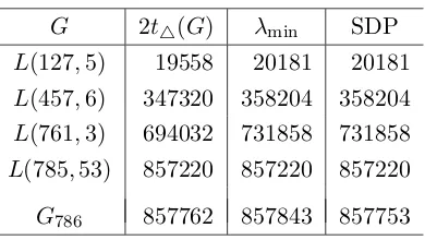
We tested all graphs from Table 1 of [105] of order less than 941 with the MAX-CUT

method, using both the minimum eigenvalue and SDP upper bounds. Table 2.4 lists the

results. Note that although none of the computed upper bounds of the L(n, s) graphs imply

arrowing (3,3), all SDP bounds match those of the minimum eigenvalue bound. This is

distinct from other families of graphs, including those in [36], as the SDP bound is usually

tighter. Thus, these graphs were given further consideration.

G 2t4(G) λmin SDP

L(127,5) 19558 20181 20181

L(457,6) 347320 358204 358204

L(761,3) 694032 731858 731858

L(785,53) 857220 857220 857220

[image:34.612.212.407.358.468.2]

G786 857762 857843 857753

Table 2.4: PotentialFe(3,3; 4) graphsGand upper bounds onM C(HG), where “λmin” is

the bound (2.1) and “SDP” is the solution of (2.4) fromSDPLR-MCandSBmethod. G786 is

the graph of Theorem 7.

Numerous attempts were made at modifying these graphs in hopes that one of the

MAX-CUT methods would be able to prove arrowing. L(127,5) was given particular attention, as

it is the same graph as G127 discussed in the previous section. Although we were unable to

obtain results with L(127,5), we were able to do so with L(785,53). Notice that all of the

upper bounds for M C(H_L₍₇₈₅_,₅₃₎) are 857220, the same as 2t4(L(785,53)). Our goal was

(35)

graph L(785,53) with one additional vertexv connected to the following 60 vertices:

{ 0, 1, 3, 4, 6, 7, 9, 10, 12, 13, 15, 16,

18, 19, 21, 22, 24, 25, 27, 28, 30, 31, 33, 34,

36, 37, 39, 40, 42, 43, 45, 46, 48, 49, 51, 52,

54, 55, 57, 58, 60, 61, 63, 66, 69, 201, 204, 207,

210, 213, 216, 219, 222, 225, 416, 419, 422, 630, 642, 645 }

These vertices were found with a simple greedy approach: v was connected to vertices 0 to

784 in order if no K4 was formed.

G786 is still K4-free, has 61290 edges, and has 428881 triangles. The upper bound

computed from the SDP solvers forM C(HG786) is 857753. We did not find a nice description

for the vectors of this solution. Software implementing SpeeDP by Grippo et al. [63],

an algorithm designed to solve large MAX-CUT SDP relaxations, was used by Rinaldi

(one of the authors of [63]) to analyze this graph. He was able to obtain the bounds

857742 ≤M C(HG786) ≤857750, which agrees with, and improves over our upper bound

computation. Since 2t4(G786) = 857762, we have both from our tests and his SpeeDPtest

that G786→(3,3), and the following main result.

Theorem 7. Fe(3,3; 4)≤786.

We note that finding a lower bound on MAX-CUT, such as the 857742≤M C(HG786)

bound from SpeeDP, follows from finding an actual cut of a certain size. This method may

be useful, as finding a cut of size 2t4(G) shows thatG6→(3,3).

2.6

Concluding Remarks

Improving the upper bound of 786 is the main challenge involved with Fe(3,3; 4). The

question of whether G127→(3,3) is still open, and any method that could solve it would be

of much interest, as it would most likely aid in deciding whether Fe(3,3; 4)<100.

Our experiments have suggested that the SDP MAX-CUT relaxation of Goemans and

Williamson produces tighter upper bounds onM C(H) than those of the minimum eigenvalue

method. This is especially apparent when H has less symmetrical structure. However, both

methods appear insufficient for further improvements to the upper bound. They both fail to

show arrowing for easy cases, such as all 659 15-vertex graphs inFe(3,3; 5) and some other

(36)

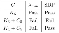
G λmin SDP

K6 Pass Pass

K3+C5 Fail Fail

[image:36.612.249.372.88.158.2]

K4+C5 Fail Pass

Table 2.5: Inconsistent results from MAX-CUT arrowing tests.

order of the graphs leaves little room for the error inherent in approximations, suggesting

that the approximations work well when the graphs are sufficiently large. This seems to

create a gap, where graphs of interest such as G127 are too small for approximation methods

like SDP-solvers but are too large for exact methods like SAT-solvers.

It is therefore likely that a new method is needed for further improvements. A possible

strategy is to attempt the computation of the exact solution of the MAX-CUT IP (2.3)

via approaches like Rendl, Rinaldi, and Wiegele’s SDP based branch & bound algorithm

[128] used in their Biq Mac software [127]. Another possible thread of work is to attempt to

prove φ(G) is unsatisfiable with methods different than exact SAT-solvers. For example,

computing an upper bound on the maximum number of satisfiable clauses can potentially

show unsatisfiability. Approximation algorithms for MAX-SAT, such as Karloff and Zwick’s

SDP based algorithm [82] and Maaren, Norden, and Heule’s sums of squares based algorithm

[139], may be worthy of investigation.

Another open question is the lower bound onFe(3,3; 4), as it is quite puzzling that only

(37)

Chapter 3

Ramsey Numbers

R

(

C

4

, K

m

)

3.1

Introduction

Let Gand H be simple graphs. Ann-vertex graph F is a (G, H;n)-graph if it contains no

subgraph isomorphic to G andF contains no subgraph isomorphic toH. Define R(G, H;n)

to be the set of all such graphs. The Ramsey number R(G, H) is the smallestnsuch that

for every two-coloring of the edges of Kn, a monochromatic copy of Gor H exists in the

first or second color, respectively. Clearly, if a (G, H;n)-graph exists, then R(G, H) > n.

It is known that Ramsey numbers exist [125] for all GandH. The values and bounds for

various types of such numbers are collected and regularly updated by Radziszowski [121].

The cycle-complete Ramsey numbers R(Cn, Km) have received much attention, both

theoretically and computationally. For fixed n = 3, the numbers are R(3, k), one of

the most studied Ramsey numbers (see [136]). Since 1976, it has been conjectured that

R(Cn, Km) = (n−1)(m−1) + 1 for all n ≥ m ≥ 3, except n = m = 3 [48, 39]. Note

that the lower bound is easy: (m−1) vertex-disjoint copies of Kn−1 provides a witness for

R(Cn, Km) >(n−1)(m−1). For over 30 years, much work has been done to verify the

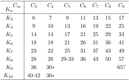
upper bound, with m= 8 being the current smallest open case. Table 3.1 presents all known

values and bounds for smallR(Cn, Km).

This work involves fixedn= 4, that is, the case of avoiding the quadrilateralC4 in the

first color. Possibly the most puzzling aspect of these numbers is that exact asymptotics are

unknown, unlike those forR(C3, Km) and related multicolored Ramsey numbers. Considering

that these numbers are a natural next step from R(C3, Kk) = R(3, k) makes them of

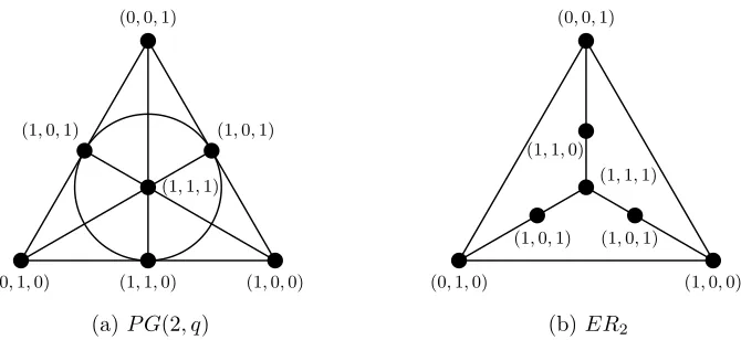
particular interest. This work focuses on values and bounds of R(C4, Km) for small m,

and the computational methods involved in enumerating (C4, Km;n)-graphs. Figure 3.1

(38)

Cm C3 C4 C5 C6 C7 C8 C9

Kn

K3 6 7 9 11 13 15 17

K4 9 10 13 16 19 22 25

K5 14 14 17 21 25 29 33

K6 18 18 21 26 31 36 41

K7 23 22 25 31 37 43 49

K8 28 26 29-33 36 43 50 57

K9 36 30∗ 65?

[image:38.612.183.436.88.246.2]

K10 40-42 36∗

Table 3.1: R(Cm, Kn) for smallmandn(this work∗). For references, see [121].

Figure 3.1: A (C4, K4; 9)-graph

the exact values for R(C4, Km) were known for 3≤m≤8. In this chapter, we present a

computational proof that R(C4, K9) = 30 and R(C4, K10) = 36.

This chapter is outlined as follows. We first discuss the known asymptotics bounds of

R(Cn, Km) and possible strategies for their improvement. Then, we discuss related topics

in extremal graph theory that involve C4-free graphs, as many such results are useful in

the study of these Ramsey numbers. We conclude with descriptions of methods for proving

values of small numbers, including our new computational results.

3.2

Asymptotics

The current best known asymptotic bounds forR(C4, Km) are,

c1

n

logn

3₂

≤R(C4, Kn)≤c2

n

logn

2

, (3.1)

wherec1 and c2 are positive constants.

[image:38.612.248.372.280.376.2]

(39)

method, which we briefly discussed in Section 2.2. The upper bound was published by Caro,

Li, Rousseau, and Zhang in 2000 [16], who in turn gave credit to an unpublished work by

Szemer´edi. The main challenge is determining whether R(C4, Kn)< n2− for some >0, a

question posed by Erd˝os in 1981 [38]. In this section, we discuss known methods that have,

or have the potential to, obtain asymptotic results for R(C4, Km).

The Probabilistic Method

The main idea behind the probabilistic method (see e.g. [4]), which was originally pioneered

by Erd˝os, involves proving that some mathematical structure exists by establishing that

theevent of such a structure existing occurs with positive probability. If there is a positive

probability that something exists, we know that it does.

An important concept used in the probabilistic method is that of thedependency digraph.

Given a collection of events A1, A2, . . . , An of some probability space Ω, the dependency

directed graph Dis defined as V(D) ={1, . . . , n} andE(D) ={(i, j)|Ai is not mutually

independent of Aj}. This graph is used in the well-known Lov´asz Local Lemma, a useful

tool of the probabilistic method proven by Erd˝os and Lov´asz in 1975 [41]. The lemma is

based on the following idea. If nmutually independent events hold with probability at least

p >0, then all events hold simultaneously with probability at least pn_>_{0, an exponentially}

small number. A generalization of this fact is the situation when events are not mutually

independent, but instead have “rare” dependencies. The goal is to still have certain events

hold with a similarly small but positive probability. Indeed, this is possible, as presented in

Lemma 1.

Lemma 1 (General Lov´asz Local Lemma, Erd˝os and Lov´asz, 1975 [41]). Given events

A1, A2, . . . , An of probability space Ωand the corresponding dependency digraph D, if there

exists x1, . . . , xn, 0≤xi <1, such that Pr(Ai)≤xiQ(i,j)∈E(D)(1−xj) for all i= 1, . . . , n,

then

Pr n

^

i=1

Ai

!

≥

n

Y

i=1

(1−xi)

The core of the proof involves the use of induction to show that for any S ⊂ {1, . . . , n},

Pr(Ai| Vj∈SAj)≤xi,i6∈S.

(40)

Theorem 8 (Spencer 1977, [134]). There exists a positive constant c such that,

R(C4, Kn)≥c

n

logn

3₂

. (3.2)

Proof. Consider an edge two-coloring of Kn where each edge is colored red and blue

randomly and independently with probabilityp and 1−p, respectively. For each set S of

four vertices, let AS be the event thatS contains a red C4. Likewise, for each set T of m

vertices, let BT be the event that all edges are blue. Clearly, R(C4, Km)> n if and only if

Pr(V

AS ∧ VBT)>0.

Note that Pr(BT) = (1−p)(

m

2) and Pr(A_S)≤6p4. Two events (either both fromA_S, both

fromBT, or one of each) are dependent if and only if the corresponding graphs share an edge.

We can then construct dependency digraphDwith vertices of allASandBT, and connecting

(in both directions) vertices according to this rule. EachASvertex is adjacent to 6 n−₂4

≤n2

other AS0 vertices and eachB_T vertex is adjacent to m 2

n−m

2

+ m₃

(n−m)≤m2n2 AS0

vertices. BothAS and BT vertices are adjacent to at most _mn

BT0 vertices.

The goal is now to find a suitable probabilityp,s, and t, all in the range [0,1), so that

we meet the condition of Lemma 1. After plugging in the probabilities and dependencies of

the events, the condition becomes

6p4 ≤s(1−s)n2(1−t)(mn)_,

and

(1−p)(m2)≤t(1−s)n 2

(1−t)(mn).

After sophisticated analysis, Spencer determined that p = c1n−2/3 and m = c2n2/3logn

work best, giving the lower bound (3.2).

Spencer used a similar argume

Solving Hard Graph Problems with Combinatorial Computing and Optimization

Theses

Recommended Citation

Dedication

Acknowledgments

Contents

Chapter 1

Background and Notation

Computational Thrust

Structure of Thesis

Chapter 2

History of

Arrowing and MAX-CUT

Experiments

Concluding Remarks

Chapter 3

Asymptotics