Article
A Comparative Study of Multiple-Criteria
Decision-Making Methods under Stochastic Inputs
Athanasios Kolios1,*, Varvara Mytilinou1, Estivaliz Lozano-Minguez2and Konstantinos Salonitis3
1 Offshore Renewable Energy Centre, Cranfield University, Cranfield MK43 0AL, UK;
2 Mechanical Engineering Research Center, Universidad Politécnica de Valencia, Valencia 46022, Spain;
3 Sustainable Manufacturing Systems Centre, Cranfield University, Cranfield MK43 0AL, UK;
* Correspondence: [email protected]; Tel.: +44-1234-75-4631
Academic Editor: Frede Blaabjerg
Received: 21 April 2016; Accepted: 7 July 2016; Published: 21 July 2016
Abstract: This paper presents an application and extension of multiple-criteria decision-making (MCDM) methods to account for stochastic input variables. More in particular, a comparative study is carried out among well-known and widely-applied methods in MCDM, when applied to the reference problem of the selection of wind turbine support structures for a given deployment location. Along with data from industrial experts, six deterministic MCDM methods are studied, so as to determine the best alternative among the available options, assessed against selected criteria with a view toward assigning confidence levels to each option. Following an overview of the literature around MCDM problems, the best practice implementation of each method is presented aiming to assist stakeholders and decision-makers to support decisions in real-world applications, where many and often conflicting criteria are present within uncertain environments. The outcomes of this research highlight that more sophisticated methods, such as technique for the order of preference by similarity to the ideal solution (TOPSIS) and Preference Ranking Organization method for enrichment evaluation (PROMETHEE), better predict the optimum design alternative.
Keywords:multi-criteria decision methods; wind turbine; support structures; weighted sum method (WSM); weighted product method (WPM); technique for the order of preference by similarity to the ideal solution (TOPSIS); analytical hierarchy process (AHP); preference ranking organization method for enrichment evaluation (PROMETHEE); elimination et choix traduisant la realité (ELECTRE); stochastic inputs
1. Introduction
Multiple-criteria decision-making (MCDM) is a procedure that combines the performance of decision alternatives across several, contradicting, qualitative and/or quantitative criteria and results in a compromise solution [1]. Relevant methods are frequently applicable, implicitly or explicitly, in numerous real-life problems and can be encountered in industrial activities where sets of decision alternatives are evaluated against conflicting criteria [2]. MCDM methods are widely used in problems within the renewable energy (RE) industry. Indicatively, methods employed include the weighted sum and weighted product methods (WSM/WPM), the analytical hierarchy process (AHP), the technique for the order of preference by similarity to the ideal solution (TOPSIS), elimination et choix traduisant la realité (ELECTRE) and the preference ranking organization method for enrichment evaluation (PROMETHEE), among others. These methods have been successfully applied in a wide
range of applications related to energy and sustainability problems [3,4]. Reference to the generic methodology behind MCDM can be found in [3,5], where one can find the most popular approaches to the most widely-applied multi-criteria methods in order to evaluate alternative solutions for real-world applications. MCDM was introduced by Saaty [6–8] and was initially developed to evaluate priorities. MCDM is very useful for policy making, new technologies and energy sources’ evaluation, being capable of incorporating both technical and non-technical attributes, i.e., economic, influencing factors [9], in the decision-making process.
Successful selection of the most appropriate multi-criteria methodology should consider a range of different perspectives in order to comprehend all sides of the problem and, when necessary, consider inter-connections among the criteria. MCDM methods need to structure the decision procedure, to demonstrate the trade-off among the criteria, to assist decision-makers to reflect upon, articulate and apply worthy judgments related to satisfactory trade-offs, resulting in suggestions when considering alternatives, to estimate risk and uncertainty more consistently and reasonably, to simplify negotiation and to keep a record of how decisions are made [10]. Real-world applications are often considered as MCDM problems; however, complications can be encountered when, for example, outlining the nature of the problem before defining the necessary alternatives, quantifying data and, finally, finding the optimum solution. Even in the seemingly simpler cases of qualitative attributes, the quality of data can be a significant source of statistical uncertainty. Further, the alternatives are derived from a wide range of choices, which are aimed at being prioritised and finally ranked or arranged in a hierarchical manner. An important issue that should be carefully considered is the fact that different attributes/criteria can cause conflicts due to their degree of completeness, redundancy, mutuality and independence, which can further complicate the decision-making process [5].
This paper aims to provide a comparative study of widely-applied MCDM methods in a real-world application and to introduce a methodology for their extension to account for stochastic inputs. An overview of selected multi-criteria methods is presented, together with a detailed analysis of the process of each method, for the easy implementation and discussion of their generic advantages and disadvantages. A case study of the selection of the optimum configuration of a support structure for a wind farm in a given location is then presented, where the criteria and alternatives of the problem are defined. Next, the data obtained through expert elicitation are presented together with the results from the implementation of each of the methods, deterministically and stochastically. A review of the results is carried out to highlight the differences and discrepancies in order to draw useful conclusions.
2. Literature Review
2.1. Review of Multiple-Criteria Decision-Making (MCDM) Methods
For the purpose of this paper, several methods have been reviewed, and eventually, the following ones have been selected, as they are the most widely applied in multi-criteria analysis problems for energy applications: WSM, WPM, TOPSIS, AHP, ELECTRE and PROMETHEE. In the next paragraphs, a brief review is given with indicative applications of each of them in the literature.
Despite the disadvantages of WSM and WPM, i.e., sensitivity to units’ ranges and exaggeration of specific scores, there are numerous applications in the literature that employ either of them primarily due to their straightforward implementation. Pilavachi et al. [19] have used an MCDM method according to a statistical estimation of weighted factors, while technical, social and economic features have also been considered. The method has been employed on the problem of risk identification and assessment within the tidal energy sector, as can be seen in [13,20], also introducing a comparison between the TOPSIS and WSM methods and showing results with good agreement.
Among many methods, TOPSIS is used extensively in different areas of research. Lozano-Minguez et al. [18] employed this deterministic methodology on the selection of the most desirable support structure of an offshore wind turbine, among three design options, under the consideration of a combination of multiple qualitative and quantitative criteria. The same concept was extended by Kolios et al. [17], where an extended version of TOPSIS is introduced, which takes into consideration the stochasticity of inputs, which is a common issue towards the successful implementation of MCDMs. With the same aim, Martin et al. [21] presented a methodology to evaluate a number of floating support structure configurations, for offshore wind turbines deployed in deep waters. Doukas et al. [22] used TOPSIS on energy policy objectives for sustainable development and renewable energy preferences, while Datta et al. [23] identified the best islanding detection method for a solar photovoltaic system by using TOPSIS along with other MCDM methods. Saelee et al. [24] employed TOPSIS as the best tool for the selection of the best among three biomass types of boiler. Finally, TOPSIS has been applied to a wide range of applications, as described in [25], where it was suggested to further investigate how to calculate the distance among positive and negative solutions.
Considering relevant applications implementing the AHP method, Kahraman and Kaya [10] implemented a fuzzy MCDM method, based on the AHP method, so as to find the optimum amongst energy policies in Turkey. Cobuloglu and Büyüktahtakιn [26] developed a new AHP-based methodology applicable to problems where uncertain data were available, and the criteria weights are identified from the MCDM case. Other applications of AHP in renewable energy-related problems can be found in [27,28], which deal with the evaluation of solar water heating systems and assessment of the local viability of renewable energy sources. AHP and the analytical network process (ANP) have been presented in [29], by using a commercial software package, so as to demonstrate the diversity of applications to which it could be employed.
Applications can certainly be found in the literature, as the use of ELECTRE is widespread. Indicatively in [30], the goal was to select the optimum site location to install an offshore wind farm among four different choices/alternatives through an innovative method based on many MCDM methods, including ELECTRE. In [31], the ELECTRE method was applied to the optimisation of decentralised energy systems. A comprehensive review of the applications of ELECTRE can be found in [32], which supports the argument that it is still an active field of research.
Continuing from the above, multi-objective optimisation (MOO) is another important MCDM method and is one of the most commonly-encountered types of optimisation problems. If there are a number of different and conflicting objectives, then the problem will fall into the category of MOO. Naturally, as a process, MOO reveals a number of non-dominated solutions [39]. A significant renewable energy-related problem is described, modelled and solved in [40], where the optimum design of switching converters was searched, in order to be integrated into related renewable technologies. The conflicting objectives were efficiency and reliability, where the optimum solution is obtained from solutions in the Pareto front. In a study on photovoltaic systems and electro-thermal methods, MOO was suggested and applied to two conflicting objectives: the maximisation of the efficiency of the solutions from Europe and their cost minimisation [41]. A lot-sizing mixed integer linear optimisation model was proposed in order to find the optimum ethanol production from several biomass sources, so as to minimise the cost and the environmentally-related issues in [42]. The trade-offs between two types of crop, i.e., food and biofuel crops, was optimised using multi-objective mixed integer programming. A model was proposed and the optimum solution obtained according to economic advantages and environmental impacts in [43]. More studies of MOO can be found in [40,44,45]. The methodology suggested by the authors in the present paper can be further applied to MOO under uncertain inputs.
2.2. Review of the Stochastic Expansion of Deterministic MCDM
A study that focused on earlier applications of MCDM methods demonstrated that developing fuzzy MCDM methods is the upcoming trend [46]. Many instances of the applications of fuzzy MCDM methods can be found in [47,48], where it was highlighted that most of the applications had selected to implement variants based on AHP. In [49], a novel fuzzy multi-actor MCDM method was used in an application of hydrogen technology, where 15 criteria were used for the sustainability assessment. In [17], during deterministic TOPSIS, the weights for each criterion were considered fixed, but under stochastic modelling, statistical distributions were employed to best fit the acquired data of the experts’ opinions. In [50,51], fuzzy VIseKriterijumska Optimizacija I Kompromisno Resenje (VIKOR) and AHP methods were applied using nine evaluation criteria for the assessment of renewable energy technologies in Turkey. The performance of several types of wind turbines was assessed in a case study in Taiwan, where the fuzzy ANP method was implemented [52]. The fuzzy ANP method was also implemented in [53], so as to mitigate the risks related to offshore wind farms, and finally, a comparison between these outcomes with the ANP and AHP methods was provided. Perera [54] has presented a study that combines MCDM and MOO in the designing process of Hybrid Energy Systems (HESs), using the fuzzy TOPSIS extension along with level diagrams. In [55], MCDM under uncertainty is discussed in an application where the alternatives’ weights are partially known. An extended and modified stochastic TOPSIS approach was implemented using interval estimations. In [56], a new stochastic-fuzzy MCDM method, called Fuzzy Stochastic Ordered Weighted Averaging (FSOWA), is presented so as to rank the alternatives and acquire the optimum alternative. The Monte Carlo method is applied to a decision-making, multi-stakeholder and hydro-environmental management case study in order to solve the uncertainty problem in [57]. A fuzzy MCDM method was also applied among energy technology alternatives so as to treat uncertainty. The AHP method under fuzziness is implemented while evaluating scores from experts [10].
3. Methodology
3.1. An Overview of Selected MCDM Methods
3.1.1. Weighted Sum Method (WSM) and Weighted Product Method (WPM)
hypothesis is applied, which implies that the overall value of every alternative is equivalent to the products’ total sum. In problems with the same units’ ranges across criteria, WSM is easily applicable; however, when the units’ ranges vary, for example when qualitative and quantitative attributes are employed, the problem becomes difficult to handle, as the aforementioned hypothesis is violated, and hence, normalisation schemes should be employed. It is common practice to use WSM along with other methods, for instance AHP, because of the method’s plain nature.
For the case ofncriteria andmalternatives, the optimum solution to the problem is obtained by the following equation:
A˚
WSM “max m ÿ
i
aijwj (1)
wherei“1, . . . ,m, A˚
WSMrepresents the weighted sum score,aijis the score of thei-th alternative with respect to thej-th criterion andwjis the weight of thej-th criterion.
An alternative to the WSM is the WPM. WPM is closely related to the WSM with the main difference being a product instead of a sum in the method. Each alternative is compared to the rest through a multiplication of ratios that are related to every criterion. Finally, WPM is considered suitable for both single and multi-dimensional cases.
This method compares alternativesAkandAlin the equation below. The optimum solution in a pairwise comparison is the one that is at least equal to the rest of the alternatives, and more specifically, the best solution isAkwhen R
´ Ak Al ¯
ą1 (when considering a maximisation problem).
R ˆ Ak Al ˙ “ n ź j“1 ˜ akj alj
¸wj
(2)
where, as previously,aijis the score of thei-th alternative with respect to thej-th criterion andwjis the weight of thej-th criterion.
3.1.2. TOPSIS
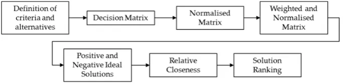
TOPSIS, depicted in Figure1, was initially proposed by Hwang et al. [58], and the idea behind it lies in the optimal alternative being as close in distance as possible from an ideal solution and at the same time as far away as possible from a corresponding negative ideal solution. Both solutions are hypothetical and are derived within the method. The concept of closeness was later established and led to the actual growth of the TOPSIS theory [59,60].
Energies 2016, 9, 566 5 of 21
attributes are employed, the problem becomes difficult to handle, as the aforementioned hypothesis
is violated, and hence, normalisation schemes should be employed. It is common practice to use
WSM along with other methods, for instance AHP, because of the method’s plain nature.
For the case of criteria and alternatives, the optimum solution to the problem is obtained
by the following equation:
∗
(1)
where 1, … , , ∗ represents the weighted sum score, is the score of the ‐th
alternative with respect to the ‐th criterion and is the weight of the ‐th criterion.
An alternative to the WSM is the WPM. WPM is closely related to the WSM with the main
difference being a product instead of a sum in the method. Each alternative is compared to the rest
through a multiplication of ratios that are related to every criterion. Finally, WPM is considered
suitable for both single and multi‐dimensional cases.
This method compares alternatives and in the equation below. The optimum solution in
a pairwise comparison is the one that is at least equal to the rest of the alternatives, and more
specifically, the best solution is when R 1 (when considering a maximisation problem).
R (2)
where, as previously, is the score of the ‐th alternative with respect to the ‐th criterion and is the weight of the ‐th criterion.
3.1.2. TOPSIS
TOPSIS, depicted in Figure 1, was initially proposed by Hwang et al. [58], and the idea behind
it lies in the optimal alternative being as close in distance as possible from an ideal solution and at
the same time as far away as possible from a corresponding negative ideal solution. Both solutions
are hypothetical and are derived within the method. The concept of closeness was later established
and led to the actual growth of the TOPSIS theory [59,60].
Figure 1. TOPSIS methodology.
After defining criteria and alternatives, the normalised decision matrix is established.
The normalised value is calculated from Equation (3), where is the ‐th criterion value for
alternative ( 1, … , and 1, … , ).
∑
(3)
The normalised weighted values in the decision matrix are calculated as follows:
(4)
The positive ideal A and negative ideal solution A are derived as shown below, where ′
[image:5.595.128.474.550.634.2]and " are related to the benefit and cost criteria (positive and negative variables).
Figure 1.TOPSIS methodology.
After defining n criteria and m alternatives, the normalised decision matrix is established. The normalised value rij is calculated from Equation (3), where fij is thei-th criterion value for alternativeAj(j“1, . . . ,mandi“1, . . . ,n).
rij“ b fij řm
j“1fij2
The normalised weighted valuesvijin the decision matrix are calculated as follows:
vij“wirij (4)
The positive ideal A`and negative ideal solution A´are derived as shown below, whereI1and I2are related to the benefit and cost criteria (positive and negative variables).
A`“ v`1, . . . ,v`n (
“ `MAXjvijˇˇiPI1 ˘
,`MI NjvijˇˇiPI2 ˘(
(5)
A´“ v´1, . . . ,v´n (
“ `MI NjvijˇˇiPI1 ˘
,`MAXjvijˇˇiPI2 ˘(
(6)
From then-dimensional Euclidean distance,D`
j is calculated in (7) as the separation of every alternative from the ideal solution. The separation from the negative ideal solution follows in (8).
D` j “ g f f e n ÿ i“1 `
vij´v`i ˘2
(7)
D´j “ g f f e n ÿ i“1 `
vij´v´i ˘2
(8)
The relative closeness to the ideal solution of each alternative is calculated from:
Cj“
D´j ´
D` j `D´j
¯ (9)
After sorting theCjvalues, the maximum value corresponds to the best solution to the problem.
3.1.3. AHP
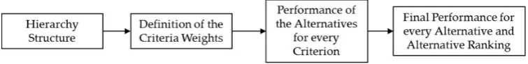
AHP was developed by Saaty [7], in 1980, and it is extensively applied in problems involving multiple, often conflicting, criteria [34]. The aim of AHP is to define the optimum alternative and to categorise the others considering the criteria that describe them. In order to apply the original AHP method, four steps should be followed, as shown in Figure2.
Energies 2016, 9, 566 6 of 21
, … , | ∈ ′ , | ∈ " (5)
, … , | ∈ ′ , | ∈ " (6)
From the ‐dimensional Euclidean distance, is calculated in (7) as the separation of every
alternative from the ideal solution. The separation from the negative ideal solution follows in (8).
(7)
(8)
The relative closeness to the ideal solution of each alternative is calculated from:
(9)
After sorting the values, the maximum value corresponds to the best solution to the problem.
3.1.3. AHP
AHP was developed by Saaty [7], in 1980, and it is extensively applied in problems involving
multiple, often conflicting, criteria [34]. The aim of AHP is to define the optimum alternative and to
categorise the others considering the criteria that describe them. In order to apply the original AHP
method, four steps should be followed, as shown in Figure 2.
Figure 2. AHP methodology.
The first phase involves the structuring of the decision problem into a hierarchical structure.
The aim is at the top of the hierarchy; the next level includes the criteria affecting the decision; and
finally, the alternatives are placed at the bottom of the hierarchy. In the second phase, the weights
for each criterion should be obtained. A pairwise comparison matrix ( ), or judgmental matrix,
should be compiled. The entry in row and column of ( ) represents how much more
important criterion is than with respect to the alternative. Saaty [7] suggested, for the
quantification of qualitative data, a scale of relative importance, i.e., the values used for any given
pair vary from 1 (where and have equal importance) to 9 (where is absolutely more
important than ). If criterion has one of the previous non‐zero numbers assigned to it when
compared to , then has the reciprocal value when compared to . reflects the importance of
the ‐th criterion and is estimated as the average of the entries in row of the matrix normalised.
Equations (10) and (11) are used to check the consistency of the pairwise comparisons.
1
(10)
where is the maximum Eigen value, is the pairwise comparison matrix and is the
weight vector.
[image:6.595.109.487.530.576.2]The Consistency Index ( ) is defined as:
Figure 2.AHP methodology.
λmax “ 1 n
n ÿ
i“1
ithentry in AWT
ithentry in WT (10)
where λmax is the maximum Eigen value, A is the pairwise comparison matrix and W is the weight vector.
The Consistency Index (CI) is defined as:
CI“ pλmaxq ´n
n´1 (11)
whereλmaxis the maximum Eigen value from the previous equation.
TheCIis then compared to the Random Index (RI) for the appropriate value ofn(Table1).
Table 1.Random Index (RI) for different values ofn[3].
n 2 3 4 5 6 7 8 9 10
RI 0 0.58 0.9 1.12 1.24 1.32 1.41 1.45 1.49
IfCI{RI> 0.10, serious inconsistencies may exist, while ifCI{RI< 0.10, the degree of consistency is considered satisfactory.
The third step refers to finding the score of each alternative for each criterion. A pairwise comparison matrix for each aim must be constructed. In the end, the best alternative (in the maximisation case) is the one that has the greatest value in the following expression:
AHPi“ n ÿ
j“1 aij řm
i“1aij
ˆ wj (12)
whereAHPiis the score of thei-th alternative, m is the number of alternatives, n is the number of the criteria,aijrepresents the actual value of thei-th alternative in terms of thej-th criterion andwjis the weight of importance of thej-th criterion.
The AHP is particularly relevant when qualitative criteria, such as environmental or political impacts, are considered. It is widely employed for energy planning problems because of its plainness and its ability to check consistency. Furthermore, throughout this method, the hierarchy is revealed after the breakdown of the problem, which enables understanding and defining the process itself. It is also suitable for dealing with technological characteristics and future aspects that are not well known [3,34]. It should be noted that AHP cannot directly consider potential associations amongst many components, as it performs poorly when different levels are independent, which implies that the method is unsuccessful in representing the complicated connections among the components. A few extensions of the AHP method have been proposed that are able to deal with these problems [61], such as the ANP method [14].
3.1.4. Elimination Et Choix Traduisant la Realité (ELECTRE)
the preferences are defined again [63]. The decision-makers are the ones to define the indifference threshold. Theoretically, there is a good reason to insert a middle area in between the indifference and the strict preference. Such a hesitation zone is regarded as a weak preference [63].
ELECTRE generates a whole system of binary outranking relations among the alternatives. Since the system may be incomplete, the preferred alternative occasionally cannot be identified. A core of leading alternatives is produced. According to this method, there is a better view of the alternatives when the least favourable choices are removed, which is particularly suitable when there are only a few criteria and many alternatives in the case [5].
As mentioned earlier, there are many variations of ELECTRE. In this study, ELECTRE I is selected, as described in [4,65], and as based on the scope and relevant literature, seems the most appropriate variation. In general two new matrices have to be created: the concordance matrix and dis-concordance matrix, as shown below:
CphSkq “ ř
jPl1wj
ř jPlwj
(13)
whereldenotes the whole set of criteria andl1 corresponds to the set of criteria that belong to the
concordant coalition, by following ELECTRE’s outranking framework.
DphSkq “ ! max j:rhjărkj
) !
rkj´rhj )
{dmax (14)
whererhjrepresents the performance of thei-th alternative against thej-th criterion anddmaxdenotes the maximal difference between the performance of alternatives.
3.1.5. Preference Ranking Organization Method for Enrichment Evaluation (PROMETHEE)
PROMETHEE is an MCDM method that was developed in 1985 [66]. Six different extensions based on the ranking were developed and used by decision-makers. First, PROMETHEE I uses partial ranking; PROMETHEE II uses complete ranking; PROMETHEE III ranks based on intervals; PROMETHEE IV is the continuous instance of the previous; PROMETHEE V includes integer linear programming and net flows; and PROMETHEE VI represents the human brain. PROMETHEE ranks the alternatives using the outranking procedure.
PROMETHEE is applied in five steps as shown in Figure3. First, the decision-maker’s preference between two actions is presented by a preference function independently. Second, the proposed set alternatives are compared between each other with respect to the preference function, and third, the comparisons’ results and the criterion’s value of each alternative are illustrated in a matrix. At the fourth step, PROMETHEE I’s approach is used so as to sort out the partial ranking, and finally, the fifth action contains the PROMETHEE II process in order to finish the alternative rankings [3].
Energies 2016, 9, 566 8 of 21
As mentioned earlier, there are many variations of ELECTRE. In this study, ELECTRE I is
selected, as described in [4,65], and as based on the scope and relevant literature, seems the most
appropriate variation. In general two new matrices have to be created: the concordance matrix and
dis‐concordance matrix, as shown below:
∑∈
∑∈ (13)
where denotes the whole set of criteria and ’ corresponds to the set of criteria that belong to the
concordant coalition, by following ELECTRE’s outranking framework.
: / (14)
where represents the performance of the i‐th alternative against the j‐th criterion and
denotes the maximal difference between the performance of alternatives.
3.1.5. Preference Ranking Organization Method for Enrichment Evaluation (PROMETHEE)
PROMETHEE is an MCDM method that was developed in 1985 [66]. Six different extensions
based on the ranking were developed and used by decision‐makers. First, PROMETHEE I uses
partial ranking; PROMETHEE II uses complete ranking; PROMETHEE III ranks based on intervals;
PROMETHEE IV is the continuous instance of the previous; PROMETHEE V includes integer linear
programming and net flows; and PROMETHEE VI represents the human brain. PROMETHEE
ranks the alternatives using the outranking procedure.
PROMETHEE is applied in five steps as shown in Figure 3. First, the decision‐maker’s preference
between two actions is presented by a preference function independently. Second, the proposed set
alternatives are compared between each other with respect to the preference function, and third, the
comparisons’ results and the criterion’s value of each alternative are illustrated in a matrix. At the
fourth step, PROMETHEE I’s approach is used so as to sort out the partial ranking, and finally, the
fifth action contains the PROMETHEE II process in order to finish the alternative rankings [3].
Figure 3. PROMETHEE methodology.
The formulae used in this implementation of PROMETHEE I are listed below, as described
in [3,67]. An important feature of PROMETHEE I is that the sum of the scores equals zero, which
informs the reader how far an alternative is from the average performance of the whole set. The
decision‐makers may select different types of criteria, which are associated with different graphical
representations of the preference function. The Type I (usual) and Type IV (level from) preference
functions are the best options for qualitative criteria, while the Type III (V‐shaped) and Type V
(linear) preference functions are the best options for quantitative criteria [68]. The choice between
them (Type I or IV; and Type III or V) will depend on whether the decision‐maker wants to
introduce an indifference threshold or not. The Type II (U‐shaped) and Type VI (Gaussian)
preference functions are used less often. The preference functions of both Types I and V are defined
below, since in the case study to follow, qualitative criteria are included.
The preference function for Type I is:
0, ∀ 0
1. ∀ 0 (15)
where denotes the numerical difference in the evaluation of two alternatives for a certain criterion.
[image:8.595.107.483.594.627.2]The preference function for Type V is:
Figure 3.PROMETHEE methodology.
The Type II (U-shaped) and Type VI (Gaussian) preference functions are used less often. The preference functions of both Types I and V are defined below, since in the case study to follow, qualitative criteria are included.
The preference function for Type I is:
ppxq “ #
0,f or@xď0
1.f or@xą0 (15)
wherexdenotes the numerical difference in the evaluation of two alternatives for a certain criterion. The preference function for Type V is:
ppxq “ $ ’ &
’ %
0, x´s
r 1,
,
f or xďs f or sďxďs`r
f or xěs`r
(16)
wheresandps`rqdenote the indifference and preference for each evaluationx. The multi-criteria preference degree is calculated from:
πpa,bq “ K ÿ
h“1
whppa,bq (17)
wherewrepresents the weight of each criterion. Outgoing flow is represented as:
Φ`p
αq “ ÿ
xPK
πpa,xq (18)
Incoming flow is defined as:
Φ´p
αq “ ÿ
xPK
πpx,aq (19)
Net flow is derived from:
Φpαq “Φ`pαq ´Φ´pαq (20)
3.2. Stochastic Expansion of Deterministic MCDM
In a real-life scenario, there are always unknown facts, which are often practically impossible to identify. For this reason, vague simplifications are often necessary in order to represent a realistic condition. The earlier researchers and practitioners used to address uncertainty by assigning numerical values to each factor and logically combining them together [69], i.e., through employing most likely values or corresponding quantiles. The term “deterministic” is related to a certain entity. Deterministic models are used to describe one out of many possible results in a reference problem. On the other hand, “stochastic” comes from the Greek “to aim” and refers to a “random” outcome. A number of potential outcomes, which are characterised by their probabilities or likelihood, is best represented through stochastic modelling. Consequently, stochastic processes denote the set of random variables that are related to a varying factor. Such processes consist of a state space, which represents the potential values, where the random variables may be related to each other [57].
A stochastic method can be more informative than a deterministic method because the former accounts for the uncertainty due to the varying behavioural characteristics of the target system. Deterministic methods are mainly used to describe simple, natural phenomena on the basis of physical laws and are not fit-for-purpose for large and complicated applications. Consequently, real-world behaviour is better reflected by employing methods relevant to stochastic simulations. The latter can include the uncertainty of real-world applications, where system modelling is not trivial. Stochastic methods can increase the confidence of the decision-maker in the final results and analysis and can be more appropriate for cases where the heterogeneity of important factors is critical as the uncertainty of the considered system increases. In general, it is not feasible to obtain an analytical expression for stochastic problems, which would require more computational time and resources to deliver a satisfactory solution [57].
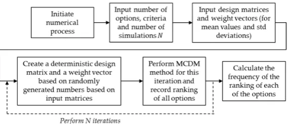
The Monte Carlo simulation method is a particularly useful approach in stochastic modelling, as it can mitigate the problems of deterministic analysis. Such an expansion of deterministic methods is developed in this paper. Principally, the Monte Carlo simulation method is an approach to represent the random nature of stochastic processes. The most fundamental part of such a method is the generation of random numbers as input sets, which are drawn randomly. Algorithms that implement the Monte Carlo simulation method consist of a sequence of finite states, a mapping function for the finite states, the probability distribution of finite states, the output space and a mapping function between the finite states and the output space [71].
The approach proposed in this paper for the stochastic expansion of deterministic methods, follows the approach proposed in [17], expanded for different methods, and is based on the fact that input variables are considered stochastically as statistical distributions that are derived by best fitting of the data collected for each value in the decision matrix and weight vector. Stochastic input data will allow Monte Carlo simulations to perform numerous iterations of analysis in order to quantify results and identify the number of cases where the optimum solution will prevail, i.e., there is aPi probability that optionXiwill rank first. Figure4. Stochastic expansion algorithm of deterministic MCDM methods illustrates the sequence of steps followed.
Energies 2016, 9, 566 10 of 21
The Monte Carlo simulation method is a particularly useful approach in stochastic modelling,
as it can mitigate the problems of deterministic analysis. Such an expansion of deterministic
methods is developed in this paper. Principally, the Monte Carlo simulation method is an approach
to represent the random nature of stochastic processes. The most fundamental part of such a method
is the generation of random numbers as input sets, which are drawn randomly. Algorithms that
implement the Monte Carlo simulation method consist of a sequence of finite states, a mapping
function for the finite states, the probability distribution of finite states, the output space and a
mapping function between the finite states and the output space [71].
The approach proposed in this paper for the stochastic expansion of deterministic methods,
follows the approach proposed in [17], expanded for different methods, and is based on the fact that
input variables are considered stochastically as statistical distributions that are derived by best
fitting of the data collected for each value in the decision matrix and weight vector. Stochastic input
data will allow Monte Carlo simulations to perform numerous iterations of analysis in order to
quantify results and identify the number of cases where the optimum solution will prevail, i.e., there
is a Pi probability that option Xi will rank first. Figure 4. Stochastic expansion algorithm of
deterministic MCDM methods illustrates the sequence of steps followed.
Figure 4. Stochastic expansion algorithm of deterministic MCDM methods.
4. Case Study
Among most of the operating offshore wind turbines installed in the Round 1 and 2 regions in
the U.K., monopile foundations have been constructed in water depths of no more than 35 m [72]
while the average water depth in an offshore wind farm in Europe was 27 m and distance from
shore 43 km, as recorded by 2016 [73,74]. Due to risk and cost limitations related to fabrication,
transportation and installation, these foundation options are not considered viable solutions in
depths that exceed 30–35 m [72], although extensive research is currently taking place to push this
boundary further. Moving further away from the shore, towards deeper waters, can lead to higher
electricity production primarily due to the higher wind shear, more available space and lower social
impact; however, deep water installations demand considerably higher volumes of materials and
installation effort, resulting in higher costs.
The advantage of fixed structures is that the designs have already been deployed in many
wind farms for years and similar concepts have been deployed for decades in the oil and gas
industry. However, fixed structures are not compatible in deeper waters because the designs
became impractical, more complicated and unsuitable for mass production. For sites that exceed the
limit of 60–70 m, the bottom‐fixed foundations encounter both technical and economic restrictions,
and it is expected that the floating wind turbine support structure concepts will become more
applicable solutions [75,76]. Currently, several floating concepts are being developed and tested in
order to qualify for scaling and further production. Floating structures still have high costs, face
issues with the footprint of the moorings, limitations for the minimum water depth in which to
operate and finally design constraints regarding the complications of volume construction.
In this case study, data were collected considering both fixed and floating structures from
[image:10.595.156.442.465.588.2]structured questionnaires from 20 experts in the wind energy field, with at least seven years’ experience
Figure 4.Stochastic expansion algorithm of deterministic MCDM methods.
4. Case Study
The advantage of fixed structures is that the designs have already been deployed in many wind farms for years and similar concepts have been deployed for decades in the oil and gas industry. However, fixed structures are not compatible in deeper waters because the designs became impractical, more complicated and unsuitable for mass production. For sites that exceed the limit of 60–70 m, the bottom-fixed foundations encounter both technical and economic restrictions, and it is expected that the floating wind turbine support structure concepts will become more applicable solutions [75,76]. Currently, several floating concepts are being developed and tested in order to qualify for scaling and further production. Floating structures still have high costs, face issues with the footprint of the moorings, limitations for the minimum water depth in which to operate and finally design constraints regarding the complications of volume construction.
In this case study, data were collected considering both fixed and floating structures from structured questionnaires from 20 experts in the wind energy field, with at least seven years’ experience in the design and implementation of RE projects. The data received were statistically processed accordingly in a preliminary study of the authors, as presented extensively in [17]. This present study aims to highlight the suitability of different MCDM methods for this problem with a view toward illustrating how well each method performs following a qualitative validation of the outcomes.
Decision Criteria and Alternatives
For this analysis, 10 design alternatives for offshore support structures are chosen, each evaluated based on 10 different criteria, listed in Tables2and3(where TLP stands for Tensioned Leg Platform). These were selected so as to extend previous work and for comparison purposes [18,21,75,77,78]. The 10 selected criteria have been qualified through a comprehensive list of 36 criteria for practicality purposes, based on semi-structured experts’ interviews and have been evaluated using qualitative variables.
‚ The compliance/maximum displacement of the rotor is considered to be a negative variable, and it represents the maximum displacement likely to be expected at the hub of the rotor that is affected by the support structure. It is treated in a different way for the floating and fixed structures; however, it does affect the rotor similarly for both structures.
‚ Dynamic performance is a positive variable, and it defines qualitatively the performance of a support structure in combination with the environmental effects and the operating loads. It is treated in a different way for the floating and fixed structures; the former has to combine the coupled effect of waves and turbine loads.
‚ Design redundancy is a positive variable, and it defines the capability to redistribute the load when a local failure is encountered.
‚ The cost of maintenance is a negative variable, and it reflects the qualitative assessment of the possible maintenance costs when, for example, any necessary equipment is involved or weather issues occur.
‚ The cost of installation is a negative variable, and it represents the qualitative assessment of the possible installation costs along with procedures, such as piling, etc.
‚ Environmental impact is a negative variable regarding the installation, operation and decommissioning impact of the foundation. Impacts on the natural environment can be considered as noise, visual, shadowing effects, disruption of the fish population’s routes, etc.
‚ Carbon footprint is a negative variable that takes into account the CO2 emissions that were
produced during all of the procedures needed for the support structure, such as the fabrication and installation processes.
‚ The likely cost is a negative variable. It represents the relative qualitative assessment of each of the concept’s costs, which, to some extent, could be quantified through the Net Present Value (NPV). ‚ Depth compatibility is a positive variable and represents the confidence levels when deploying
a concept, which considers current installations for any applications with respect to a reference depth.
[image:12.595.184.412.309.442.2]A Likert scale has been employed in the questionnaires in order to provide uniform input data. The experts were asked to identify their level of agreement or disagreement using a number from within the 1–9 scores, as the Likert scale suggests. The scale usually states nine as the most critical response. The same 1–9 scales was used to rank the different alternatives that correspond to the design criteria. According to the positive or negative nature of the criteria, nine and one are the optima, respectively. Although usually in practice, the Likert scale is defined through a 1–5 scale, due to the fact that statistical processing has followed the collection of the data, a broader range of values was deemed more appropriate.
Table 2.List of criteria.
ID Decision Criterion
A Compliance/Max Displacement of Rotor
B Dynamic Performance
C Design Redundancy
D Cost of Maintenance
E Cost of Installation
F Environmental Impact
G Carbon Footprint
H Certification
I Likely Cost
J Depth Compatibility
Table 3.List of alternatives.
ID Decision Alternative
A1 Jacket
A2 Tripod
A3 Monopile
A4 Suction Bucket
A5 Jack-up
A6 Spar
A7 Barge
A8 TLP
A9 Semi-Submersible
A10 Tri-floater
In order to define the problem, a relatively large-scale wind turbine (such as 5.5 MW) was considered to be installed in a 40-m water depth, and 10 design configurations were proposed for the support structure against the 10 selected criteria. The depth is considered to be a key parameter of the problem, as it is expected that it will influence the final outcome based on the experts’ responses. The designs included five fixed and five floating support options.
All design alternatives have both advantages and disadvantages, and that is the reason behind the proposed criteria and how their aggregation can qualify as the best performance. Several more support structures can be found in the literature, including some concepts that combine different types’ features in a single design. These types usually have some advantages, overcoming some of the problems, and are suitable for a wide range of water depths. These hybrid structures are outside the scope of this paper, but could be investigated further in the future; however, the approach suggested in this paper is applicable for their assessment.
[image:12.595.219.376.476.610.2]5. Results and Discussion
5.1. Deterministic Results
The results of the deterministic application of the MCDM methods are presented in this section. In the context of this application, certain criteria had to be maximised, and others had to be minimised. Here, only maximisation is considered, and any criteria for minimisation are multiplied by´1, where relevant. Most of the methods provide absolute scores, which are used for ordering the solutions at the end. Since maximisation is considered, the score should be as high as possible. When a method generates a pairwise solution, the solution that outperforms most of the other alternatives is considered to be the optimum.
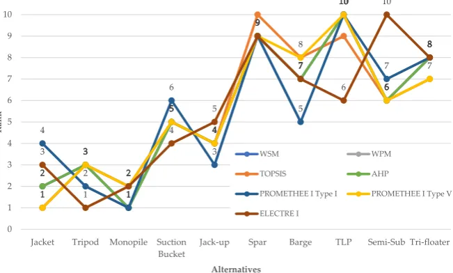
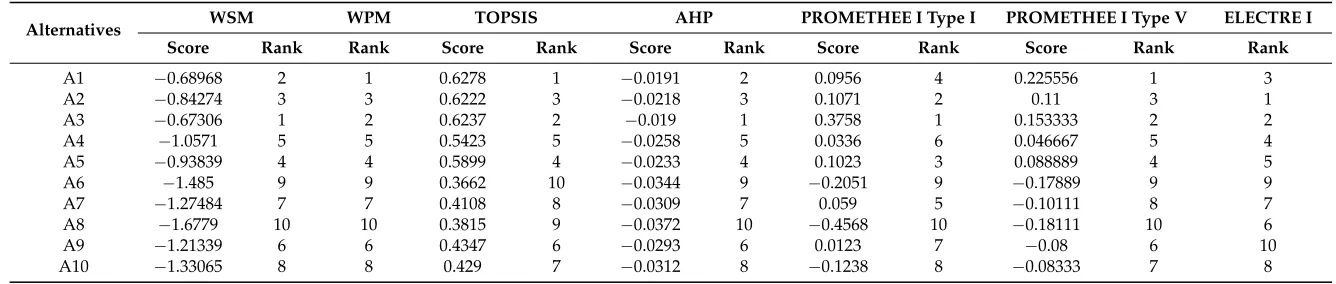
As can be seen from Figure5, in most cases, the methods derive close optimum solutions. Table5 summarises the WSM, WPM, TOPSIS, AHP, PROMETHEE I and ELECTRE I results and ranking.Energies 2016, 9, 566 13 of 21
Figure 5. Ranks comparison for the WSM, WPM, TOPSIS, AHP, PROMETHEE I and ELECTRE I methods.
In more detail:
WSM: This has been the simplest method applied, and the result for the optimal solution is
Alternative A3, the monopile design, followed by A1 (jacket) as the second option.
WPM: WPM generates a matrix with pairwise comparison performance, as shown in Table 6.
Hence, in this case, A1 (jacket) is superior to all of the other alternatives, because the ratio is
higher than one in all cases. Following this, the monopile stands as the second best option.
TOPSIS: According to this method, again, the jacket (A1) design achieves the highest score
followed by the monopile concept.
AHP: This method ranks the monopile (A3) design highest, followed by the jacket. The final
ranking seems to be closer to the rest of the methods, and this can be explained due to the
similarity of this method to the WSM.
PROMETHEE I: Two different types of criteria were employed for the PROMETHEE I method.
First, the Type I preference function was applied, and the monopile (A3) was found to be the
best alternative in this case. Second, the results from the Type V preference function indicate
that the jacket design achieves the highest score (A1).
ELECTRE I: As a result, this method generates two matrices, which cumulatively qualify the
tripod (A2) as the best option followed by the monopile and jacket. 2 3 1 5 4 9 7 10 6 8 1 3 2 5 4 9 7 10 6 8 2 3 1 5 4 9 7 10 6 8 4 2 1 6 3 9 5 10 7 8 1 3 2 5 4 9 8 10 6 7 3 1 2 4 5 9 7 6 10 8 0 1 2 3 4 5 6 7 8 9 10
Jacket Tripod Monopile Suction Bucket
Jack‐up Spar Barge TLP Semi‐Sub Tri‐floater
Rank
Alternatives
WSM WPM
TOPSIS AHP
PROMETHEE I Type I PROMETHEE I Type V
[image:13.595.136.462.269.465.2]ELECTRE I
Figure 5. Ranks comparison for the WSM, WPM, TOPSIS, AHP, PROMETHEE I and ELECTRE I methods.
In more detail:
‚ WSM: This has been the simplest method applied, and the result for the optimal solution is Alternative A3, the monopile design, followed by A1 (jacket) as the second option.
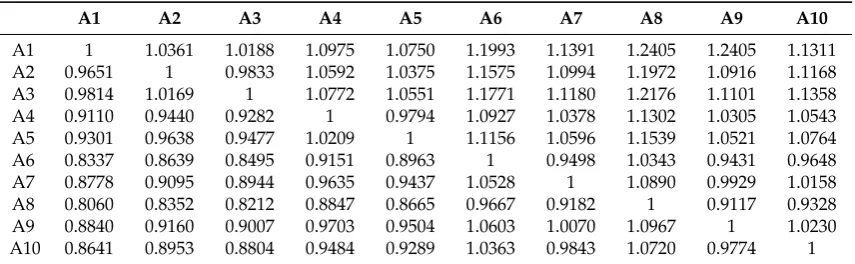
‚ WPM: WPM generates a matrix with pairwise comparison performance, as shown in Table6. Hence, in this case, A1 (jacket) is superior to all of the other alternatives, because the ratio is higher than one in all cases. Following this, the monopile stands as the second best option.
‚ TOPSIS: According to this method, again, the jacket (A1) design achieves the highest score followed by the monopile concept.
‚ AHP: This method ranks the monopile (A3) design highest, followed by the jacket. The final ranking seems to be closer to the rest of the methods, and this can be explained due to the similarity of this method to the WSM.
‚ PROMETHEE I: Two different types of criteria were employed for the PROMETHEE I method. First, the Type I preference function was applied, and the monopile (A3) was found to be the best alternative in this case. Second, the results from the Type V preference function indicate that the jacket design achieves the highest score (A1).
Table 4.Mean evaluation values (design matrix) and normalised mean values of the weights.
Alternatives/Criteria
Compliance/ Max Displacement
of Rotor
Dynamic Performance
Design Redundancy
Cost of Maintenance
Cost of Installation
Environmental Impact
Carbon
Footprint Certification Likely Cost
Depth Compatibility
Jacket 1.6 7.7 7.8 5.9 6.6 7.4 6.6 7.7 5.7 7.7
Tripod 2 7.2 6.3 5.8 6.2 6.9 6.2 7.2 5.3 7
Monopile 2.7 6.5 5.7 4.7 5.9 6.5 5.2 7.8 4.4 6.1
Suction Bucket 3.3 6.1 5 5 5.3 6.5 5.1 5.9 4.5 5.3
Jack-up 3.2 6.6 6.1 5.4 4.6 5 5.9 6.8 7 6.4
Spar 5.8 5.9 5.1 4.8 4.8 3.6 5.3 5.4 6.5 3.9
Barge 6.6 4.6 5.3 4.6 3.8 3.4 5.3 5.2 5.9 5.6
TLP 4.2 6.6 4.4 5.7 5.6 5.2 6 5.5 7.3 5
Semi-Submersible 5.6 5.8 5.3 4.6 4.2 3.7 5.9 5.6 6.7 5.9
Tri-floater 5.5 5.7 4.9 5 3.9 3.5 5.7 4.3 6.4 5.7
Normalised weight values 0.11 0.09 0.09 0.13 0.12 0.08 0.07 0.09 0.13 0.10
Table 5.WSM, TOPSIS, AHP, PROMETHEE I and ELECTRE I results and rank.
Alternatives WSM WPM TOPSIS AHP PROMETHEE I Type I PROMETHEE I Type V ELECTRE I
Score Rank Rank Score Rank Score Rank Score Rank Score Rank Rank
A1 ´0.68968 2 1 0.6278 1 ´0.0191 2 0.0956 4 0.225556 1 3
A2 ´0.84274 3 3 0.6222 3 ´0.0218 3 0.1071 2 0.11 3 1
A3 ´0.67306 1 2 0.6237 2 ´0.019 1 0.3758 1 0.153333 2 2
A4 ´1.0571 5 5 0.5423 5 ´0.0258 5 0.0336 6 0.046667 5 4
A5 ´0.93839 4 4 0.5899 4 ´0.0233 4 0.1023 3 0.088889 4 5
A6 ´1.485 9 9 0.3662 10 ´0.0344 9 ´0.2051 9 ´0.17889 9 9
A7 ´1.27484 7 7 0.4108 8 ´0.0309 7 0.059 5 ´0.10111 8 7
A8 ´1.6779 10 10 0.3815 9 ´0.0372 10 ´0.4568 10 ´0.18111 10 6
A9 ´1.21339 6 6 0.4347 6 ´0.0293 6 0.0123 7 ´0.08 6 10
[image:14.842.86.754.295.437.2]Table 6.WPM pairwise comparison matrix.
A1 A2 A3 A4 A5 A6 A7 A8 A9 A10
A1 1 1.0361 1.0188 1.0975 1.0750 1.1993 1.1391 1.2405 1.2405 1.1311 A2 0.9651 1 0.9833 1.0592 1.0375 1.1575 1.0994 1.1972 1.0916 1.1168 A3 0.9814 1.0169 1 1.0772 1.0551 1.1771 1.1180 1.2176 1.1101 1.1358 A4 0.9110 0.9440 0.9282 1 0.9794 1.0927 1.0378 1.1302 1.0305 1.0543 A5 0.9301 0.9638 0.9477 1.0209 1 1.1156 1.0596 1.1539 1.0521 1.0764 A6 0.8337 0.8639 0.8495 0.9151 0.8963 1 0.9498 1.0343 0.9431 0.9648 A7 0.8778 0.9095 0.8944 0.9635 0.9437 1.0528 1 1.0890 0.9929 1.0158 A8 0.8060 0.8352 0.8212 0.8847 0.8665 0.9667 0.9182 1 0.9117 0.9328 A9 0.8840 0.9160 0.9007 0.9703 0.9504 1.0603 1.0070 1.0967 1 1.0230 A10 0.8641 0.8953 0.8804 0.9484 0.9289 1.0363 0.9843 1.0720 0.9774 1
Jacket qualifies as the best alternative for WPM, TOPSIS and PROMETHEE I Type V, while monopile is the best alternative for WSM, AHP and PROMETHEE I Type I. From experience, it would be expected that these two concepts would score higher, as their implementation would introduce lower risk, as they are the most widely-used concepts to date [74]. Although the applicability boundaries of monopiles are pushed to account for deeper waters in order to take advantage of their ease in fabrication and installation, the threshold of 35 m would still face challenges to be achieved due to practical, technical difficulties [79–81]. Hence, the jacket would be expected to be the prevailing concept for this problem.
It is not surprising that WSM, AHP and PROMETHEE I Type I methods consider the monopile as the best alternative, since they are the least sophisticated methods among those evaluated. The maintenance and likely costs, which have a negative nature, are the criteria that obtained the highest values for the vector weight, and for both of them, the monopile has a much lower score than the jacket; hence, it can be concluded that the effect of these extreme scores has been underestimated by using these less sophisticated methods. Results obtained from the deterministic application of the different methods employed in this paper can be supported by the findings of other studies for similar problems comparing different MCDM methods, i.e., [82–84].
5.2. Stochastic Results
Figure 6. Comparative stochastic MCDM results: probability of an alternative to score first.
From the results of the stochastic analysis, it can be observed that Alternatives A1, A2 and A3
(jacket, tripod and monopile) consistently perform better than the rest with probabilities of ranking
first between 49.4% (ELECTRE I) and 71.1% (PROMETHEE I TYPE V). Comparing fixed with
floating options, the former rank higher with probabilities between 67.5% (ELECTRE I) and 83.7%
(AHP). It should be noted that the PROMETHEE I TYPE V exaggerates in the prediction of the
optimum alternative and presents some relative inconsistency with respect to the others, while
ELECTRE I also seems to be mis‐ranking the least optimum options; hence, these methods seem to
be less suitable for the reference application.
Table 7. Stochastic WSM, TOPSIS, AHP, PROMETHEE I and ELECTRE I results.
Alternatives WSM WPM TOPSIS AHP PROMETHEE TYPE V
PROMETHEE
I TYPE I ELECTRE I A1 21.64% 21.94% 18.12% 21.62% 47.75% 22.09% 27.33%
A2 14.39% 14.34% 14.40% 14.40% 17.26% 15.27% 15.80%
A3 25.62% 23.59% 24.09% 25.16% 6.07% 23.07% 6.24%
A4 11.30% 12.19% 12.84% 11.43% 2.67% 9.81% 3.55%
A5 10.35% 8.73% 11.58% 11.13% 9.62% 10.41% 14.59%
A6 3.37% 4.29% 3.73% 3.31% 2.75% 3.80% 4.96%
A7 4.65% 6.04% 5.11% 4.28% 1.09% 5.65% 3.01%
A8 1.24% 1.64% 2.14% 1.60% 8.92% 1.13% 12.84%
A9 4.83% 4.27% 4.88% 4.57% 2.94% 5.56% 7.90%
A10 2.60% 2.97% 3.11% 2.50% 0.93% 3.20% 3.79%
The results above are countersigned by current practice as fixed support structures, and
particularly, monopiles and jackets have reached far higher Technology Readiness Level (TRL) than
floating concepts, which are still to achieve full commercialisation due to the various risks associated
with their wider implementation (i.e., design for volume production, cost of moorings, dynamic
performance, etc.). It should also be observed that the definition of the problem, referring to a 40‐m
depth deployment, consists of a determining factor of this conclusion, as it is expected that for the
case of a deeper installation (i.e., 70 m), fixed concepts would have scored much lower in the criteria
of cost of maintenance, cost of installation, certification, likely cost and depth compatibility.
0% 5% 10% 15% 20% 25% 30% 35% 40% 45% 50%
Jacket Tripod Monopile Suction
Bucket
Jack‐up Spar Barge TLP Semi‐Sub Tri‐floater
%
Proba
b
ility
Alternatives
WSM WPM
TOPSIS AHP
PROMETHEE I TYPE V PROMETHEE I TYPE I
[image:16.595.117.477.92.301.2]ELECTRE I
Figure 6.Comparative stochastic MCDM results: probability of an alternative to score first.
From the results of the stochastic analysis, it can be observed that Alternatives A1, A2 and A3 (jacket, tripod and monopile) consistently perform better than the rest with probabilities of ranking first between 49.4% (ELECTRE I) and 71.1% (PROMETHEE I TYPE V). Comparing fixed with floating options, the former rank higher with probabilities between 67.5% (ELECTRE I) and 83.7% (AHP). It should be noted that the PROMETHEE I TYPE V exaggerates in the prediction of the optimum alternative and presents some relative inconsistency with respect to the others, while ELECTRE I also seems to be mis-ranking the least optimum options; hence, these methods seem to be less suitable for the reference application.
Table 7.Stochastic WSM, TOPSIS, AHP, PROMETHEE I and ELECTRE I results.
Alternatives WSM WPM TOPSIS AHP PROMETHEE
TYPE V
PROMETHEE
I TYPE I ELECTRE I
A1 21.64% 21.94% 18.12% 21.62% 47.75% 22.09% 27.33%
A2 14.39% 14.34% 14.40% 14.40% 17.26% 15.27% 15.80%
A3 25.62% 23.59% 24.09% 25.16% 6.07% 23.07% 6.24%
A4 11.30% 12.19% 12.84% 11.43% 2.67% 9.81% 3.55%
A5 10.35% 8.73% 11.58% 11.13% 9.62% 10.41% 14.59%
A6 3.37% 4.29% 3.73% 3.31% 2.75% 3.80% 4.96%
A7 4.65% 6.04% 5.11% 4.28% 1.09% 5.65% 3.01%
A8 1.24% 1.64% 2.14% 1.60% 8.92% 1.13% 12.84%
A9 4.83% 4.27% 4.88% 4.57% 2.94% 5.56% 7.90%
A10 2.60% 2.97% 3.11% 2.50% 0.93% 3.20% 3.79%
The results above are countersigned by current practice as fixed support structures, and particularly, monopiles and jackets have reached far higher Technology Readiness Level (TRL) than floating concepts, which are still to achieve full commercialisation due to the various risks associated with their wider implementation (i.e., design for volume production, cost of moorings, dynamic performance, etc.). It should also be observed that the definition of the problem, referring to a 40-m depth deployment, consists of a determining factor of this conclusion, as it is expected that for the case of a deeper installation (i.e., 70 m), fixed concepts would have scored much lower in the criteria of cost of maintenance, cost of installation, certification, likely cost and depth compatibility.
[image:16.595.79.517.482.611.2]the floating concepts, spar, barge and TLP outperform the tri-floater and semi-sub. These findings illustrate that the stochastic approach proposed in this paper is able to evaluate the relative risks encountered with the selection of each of the chosen options.
6. Conclusions
The application of MCDM methods in engineering problems and particularly those related to renewable energy applications, can provide useful insight for decision-makers towards more qualified decisions. The present study demonstrated the application of six MCDM methods that are frequently used on numerous renewable energy applications, namely WSM, WPM, TOPSIS, AHP, PROMETHEE I and ELECTRE I, and their extension to consider stochastic inputs and assign confidence levels in the resulting outputs.
For the reference case study, 10 significant technical and non-technical criteria were employed to assess the optimal solution among 10 different alternatives of support structures for offshore wind turbines. After applying the MCDM methods on the case deterministically, it can be concluded that most methods agree on identifying the set with the highest score, with the most sophisticated methods, i.e., TOPSIS and PROMETHEE, more accurately predicting the jacket type configuration as the prevailing one, followed by the monopile. The expansion of the methods to account for uncertain inputs has shown similar results, qualifying the fixed concepts and, in particular, the jacket, tripod and monopile, as the prevailing options. A reasonable agreement can be observed among the methods, with the exceptions of PROMETHEE I TYPE V and ELECTRE I, which seem less suitable for this purpose, as they misjudge the ranking of the less optimal options. It should be noted here that a conclusion cannot be generalised, i.e., that one method outperforms the rest, as accuracy in prediction depends on the nature of the problem, as well as the data collection and processing in a way that best fits each individual method and application.
Acknowledgments: This work was supported by Grant EP/L016303/1 for Cranfield University, Centre for Doctoral Training in Renewable Energy Marine Structures (REMS) (http://www.rems-cdt.ac.uk/) from the U.K. Engineering and Physical Sciences Research Council (EPSRC).
Conflicts of Interest:The authors declare no conflict of interest.
References
1. Dadda, A.; Ouhbi, I. A decision support system for renewable energy plant projects. In Proceedings of the 2014 Fifth International Conference on Next Generation Networks and Services (NGNS), Casabalanca, Morocco, 28–30 May 2014.
2. Triantaphyllou, E.; Mann, S.H. Using the analytic hierarchy process for decision making in engineering applications: Some challenges.Int. J. Ind. Eng. Appl. Pract.1995,2, 35–44.
3. Mateo, J.R.S.C.Multi-Criteria Analysis in the Renewable Energy Industry; Springer-Verlag: London, UK, 2012. 4. Rogers, M.; Bruen, M.; Maystre, L.-Y.ELECTRE and Decision Support, Methods and Applications in Engineering
and Infrastructure Investment; Springer Science+Business Media, LLC: New York, NY, USA, 2000.
5. Triantaphyllou, E.; Shu, S.; Sanchez, S.N.; Ray, T. Multi-criteria decision making: An operations research approach.Encycl. Electr. Electron. Eng.1998,15, 175–186.
6. Saaty, T.L.Decision Making with Dependence and Feedback: The Analytic Network Process; RWS Publications: Pittsburgh, PA, USA, 1996; Volume 4922.
7. Saaty, T.L.The Analytic Hierarchy Process: Planning, Priority Setting, Resources Allocation; McGraw-Hill: New York, NY, USA, 1980.
8. Saaty, T.L. What is the analytic hierarchy process? InMathematical Models for Decision Support; Mitra, G., Greenberg, H.J., Lootsma, F.A., Rijkaert, M.J., Zimmermann, H.J., Eds.; Springer: Berlin/Heidelberg, Germany, 1988; pp. 109–121.
10. Kahraman, C.; Kaya, ˙I. A fuzzy multicriteria methodology for selection among energy alternatives. Exp. Syst. Appl.2010,37, 6270–6281. [CrossRef]
11. Mardani, A.; Jusoh, A.; Zavadskas, E.K.; Cavallaro, F.; Khalifah, Z. Sustainable and renewable energy: An overview of the application of multiple criteria decision making techniques and approaches.Sustainability
2015,7, 13947–13984. [CrossRef]
12. Peng, J.-J.; Wang, J.Q.; Wang, J.; Yang, L.J.; Chen, X.H. An extension of ELECTRE to multi-criteria decision-making problems with multi-hesitant fuzzy sets.Inf. Sci.2015,307, 113–126. [CrossRef]
13. Kolios, A.; Read, G.; Ioannou, A. Application of multi-criteria decision-making to risk prioritisation in tidal energy developments.Int. J. Sustain. Energy2016,35, 59–74. [CrossRef]
14. Shafiee, M.; Kolios, A.J. A multi-criteria decision model to mitigate the operational risks of offshore wind infrastructures. In Proceedings of the European Safety and Reliability Conference, ESREL 2014, Wroclaw, Poland, 14–18 September 2014; CRC Press/Balkema: Wroclaw, Poland, 2015.
15. Govindan, K.; Rajendran, S.; Sarkis, J.; Murugesan, P. Multi criteria decision making approaches for green supplier evaluation and selection: A literature review.J. Clean. Prod.2013,98, 66–83. [CrossRef]
16. Mourmouris, J.C.; Potolias, C. A multi-criteria methodology for energy planning and developing renewable energy sources at a regional level: A case study thassos, greece.Energy Policy2013,52, 522–530. [CrossRef] 17. Kolios, A.J.; Rodriguez-Tsouroukdissian, A.; Salonitis, K. Multi-criteria decision analysis of offshore wind
turbines support structures under stochastic inputs.Ships Offshore Struct.2016,11, 38–49.
18. Lozano-Minguez, E.; Kolios, A.J.; Brennan, F.P. Multi-criteria assessment of offshore wind turbine support structures.Renew. Energy2011,36, 2831–2837. [CrossRef]
19. Pilavachi, P.; Roumpeas, C.P.; Minett, S.; Afgan, N.H. Multi-criteria evaluation for CHP system options. Energy Convers. Manag.2006,47, 3519–3529. [CrossRef]
20. Kolios, A.; Read, G. A political, economic, social, technology, legal and environmental (PESTLE) Approach for risk identification of the tidal industry in the United Kingdom.Energies2013,6, 5023–5045. [CrossRef] 21. Martin, H.; Spano, G.; Küster, J.F.; Collu, M.; Kollios, A.J. Application and extension of the TOPSIS method
for the assessment of floating offshore wind turbine support structures.Ships Offshore Struct.2013,8, 477–487. [CrossRef]
22. Doukas, H.; Karakosta, C.; Psarras, J. Computing with words to assess the sustainability of renewable energy options.Exp. Syst. Appl.2010,37, 5491–5497. [CrossRef]
23. Datta, A.; Saha, D.; Ray, A.; Das, P. Anti-islanding selection for grid-connected solar photovoltaic system applications: A MCDM based distance approach.Solar Energy2014,110, 519–532. [CrossRef]
24. Saelee, S.; Paweewan, B.; Tongpool, R.; Witoon, T.; Takada, J.; Manusboonpurmpool, K. Biomass type selection for boilers using TOPSIS multi-criteria model.Int. J. Environ. Sci. Dev.2014,5, 181–186. [CrossRef] 25. Behzadian, M.; Otaghsara, S.K.; Yazdani, M.; Ignatius, J. A state-of the-art survey of TOPSIS applications.
Exp. Syst. Appl.2012,39, 13051–13069. [CrossRef]
26. Cobuloglu, H.I.; Büyüktahtakın, ˙I.E. A stochastic multi-criteria decision analysis for sustainable biomass crop selection.Exp. Syst. Appl.2015,42, 6065–6074. [CrossRef]
27. Mohsen, M.S.; Akash, B.A. Evaluation of domestic solar water heating system in jordan using analytic hierarchy process.Energy Convers. Manag.1997,38, 1815–1822. [CrossRef]
28. Nigim, K.; Munier, N.; Green, J. Pre-feasibility MCDM Tools to aid communities in prioritizing local viable renewable energy sources.Renew. Energy2004,29, 1775–1791. [CrossRef]
29. Saaty, R.W.Decision Making in Complex Environments: The Analytic Hierarchy Process (AHP) for Decision Making and the Analytic Network Process (ANP) for Decision Making with Dependence and Feedback; Super Decisions: Pittsburgh, PA, USA, 2003.
30. Fetanat, A.; Khorasaninejad, E. A novel hybrid MCDM approach for offshore wind farm site selection: A case study of Iran.Ocean Coast. Manag.2015,109, 17–28. [CrossRef]
31. Papadopoulos, A.; Karagiannidis, A. Application of the multi-criteria analysis method electre III for the optimisation of decentralised energy systems.Omega2008,36, 766–776. [CrossRef]
32. Govindan, K.; Jepsen, M.B. ELECTRE: A comprehensive literature review on methodologies and applications. Eur. J. Oper. Res.2016,250, 1–29. [CrossRef]