The commitment problem of secured lending

      

City, University of London Institutional Repository

Citation:

Fabbri, D. & Menichini, A.M.C. (2016). The commitment problem of secured lending. Journal of Financial Economics, 120(3), pp. 561-584. doi:

10.1016/j.jfineco.2016.02.009

This is the accepted version of the paper.

This version of the publication may differ from the final published

version.

Permanent repository link:

http://openaccess.city.ac.uk/17180/

Link to published version:

http://dx.doi.org/10.1016/j.jfineco.2016.02.009

Copyright and reuse: City Research Online aims to make research

outputs of City, University of London available to a wider audience.

Copyright and Moral Rights remain with the author(s) and/or copyright

holders. URLs from City Research Online may be freely distributed and

linked to.

The Commitment Problem of Secured Lending

Daniela Fabbri∗

Cass Business School

Anna Maria C. Menichini†

University of Salerno and CSEF

September 2015

Abstract

The paper presents a new theory of trade credit where firms buy inputs on credit from suppliers to restore the benefits of secured bank financing impaired by contract incompleteness. In a setting where investment is endogenous and unobservable to financiers, we show that a bank-secured credit contract is time-inconsistent: Upon being granted credit, the entrepreneur has an incentive to alter the original input combination, jeopardizing the bank’s revenues. Anticipating the entrepreneur’s opportunism, the bank offers an unsecured credit contract, reducing the surplus from the venture. One way for the entrepreneur to commit to the contract terms is to purchase inputs on credit from the supplier. The supplier observes the input investment and acts as a guarantor that inputs will be purchased as contracted, thus facilitating access to secured bank financing. The commitment role of trade credit still holds in a multi-period extension that investigates the impact of bank relationship lending on secured debt and trade credit. Our model provides novel testable predictions on optimal financial contracts in both one-period and repeated-lending relationships.

Keywords: collateral, commitment, trade credit, bank financing.

JEL classification: G32, G33, K22, L14.

∗

Contact address: Faculty of Finance, Cass Business School, 106 Bunhill Row, London, EC1Y 8TZ, UK. Tel.: +44 (0)20 7040 0966. Fax.: +44 (0)20 7040 8881. E-mail: [email protected]

†

Introduction

Firms procure funds not only from specialized financial intermediaries but also from suppliers, which

generally delay payments of inputs. Trade credit is an important source of external financing for

firms of all sizes across both developed and developing countries (Petersen and Rajan, 1997; Beck,

Demirg¨u¸c-Kunt, and Maksimovic, 2008; Giannetti , Burkart, and Ellingsen, 2011) and across both

domestic and foreign markets (Auboin and Engeman, 2014; Manova, 2013). Researchers have mostly

rationalized and documented the substitution effect of trade credit, arguing that firms rely on trade

credit when they are constrained on bank financing (e.g., Calomiris, Himmelberg, and Wachtel, 1995;

Petersen and Rajan, 1997; Burkart and Ellingsen, 2004; Love, Preve, and Sarria Allende, 2007; among

others). Recent empirical evidence, however, indicates that the complementarity effects of trade credit

are also relevant. Giannetti, Burkart, and Ellingsen (2011) show that U.S. firms obtaining credit from

suppliers can secure financing from relatively uninformed banks. Garcia-Appendini (2010) documents

that small, non-financial firms in the U.S. are more likely to secure bank credit if they have been

granted trade credit from their suppliers.1

We propose a new theory of trade credit that can be used to explain these stylized facts. Firms buy

capital inputs on account to restore the benefits of secured bank financing impaired by the borrower’s

inability to credibly commit to investment in pledgeable assets. We show that if the investment in

a given asset is not contractible, pledging it as collateral fails to increase external financing. This is

because collateral introduces a problem of moral hazard in the form of asset substitution (i.e., the

entrepreneur has an ex post incentive to alter the input mix), making secured bank credit unfeasible.

We show that the entrepreneur can use trade credit to mitigate this problem. It follows that when

investment is non-contractible, buying inputs on account facilitates access to secured bank lending.2

We construct a one-period model where an entrepreneur produces a good for with uncertain

demand. The entrepreneur uses two inputs, capital and labor, whose purchase is entirely financed

by external financiers. The inputs have different collateral values. For simplicity, only capital can

be pledged to financiers. Being specialized financial intermediaries, banks typically offer the cheapest

source of financing. If banks observe the amount of inputs purchased and thus invested, the optimal

1

Cook (1999) documents that accounts payable raise the likelihood of a Russian firm obtaining a bank loan. Alphonse, Ducret, and Severin (2006) document that the more trade credit U.S. firms use, the more indebted they are to banks, more so for firms with short-term banking relationships. Along the same lines, Gama, Mateus, and Teixera (2010) find that the use of payables allows younger and smaller firms in Spain and Portugal to increase the availability of bank financing.

2

contract is secured debt. The input combination is tilted towards capital, which is fully pledged as

collateral. Collateral gives the bank protection against losses in default, thereby increasing the amount

of external financing and the total surplus of the lending relation. However, the value of the collateral is

not exogenous - it can be affected by the borrower’s input choice. So, if the investment is not observable,

upon receiving the bank loan, the entrepreneur has an incentive to alter the original input combination

towards the input with the lowest collateral value and higher productivity. This jeopardizes the bank’s

expected revenues by reducing the liquidation income in case of default. Anticipating that it will not

break even, the bank abandons the secured contract, thus causing an efficiency loss.

One way to avoid this is for the entrepreneur to purchase the capital input on credit and pledge it to

the supplier in case of default. As the provider of the input, the supplier observes the input investment.

Knowing the investment level and having a stake in the default state, he implicitly guarantees purchase

of the quantity of inputs specified in the financial contracts, and thus available for liquidation to all

creditors, thereby restoring the benefits of secured bank financing.

This commitment effect of trade credit is robust to the possibility of a costly collusive

agreement between the entrepreneur and the supplier and to repeated entrepreneur-bank interactions.

Specifically, we extend our static baseline model to a multi-period setting to investigate how trade

credit and secured debt are affected by relationship lending, i.e., a long-term contract with credit

amounts and repayment obligations contingent on some information about the borrower’s past behavior

(e.g., Boot and Thakor, 1994; 2000). We show that trade credit is still the best way to solve the

commitment problem if projects are not too lengthy. We also find that entrepreneurs are more likely

to use trade credit than relationship lending when inputs have high collateral value and low-quality

information is collected by the relationship lender.

In practice, entrepreneurs largely use secured loans, many of which are sensitive to the commitment

problem. Asset-based lending (ABL) is one important source of short-term financing (typically with

a three-year maturity) that many firms in the U.S. and Canada use to fund their working capital. In

2002, ABL in the U.S. was $326 billion, almost a quarter of total short-term credit, which increased to

$590 billion in 2008.3 In ABL, the bank lends funds to a firm in exchange for collateral, which generally

includes equipment, small machinery, inventory, and accounts receivable. Since the value of the asset

pledged as collateral is clearly affected by input purchases that are not easily observable by the bank,

ABL is particularly vulnerable to the commitment problem analyzed in this paper. Moreover, the

firm likely purchases most of these assets on credit, which is consistent with our theoretical setting.

Our model is less suited for situations where the assets pledged as collateral are registered, such as in

real estate-based lending.4 However, even in these cases, the 2007-2009 financial crisis demonstrated

that there were instances in which creditors were unable to identify ex ante the appropriate value

of the collateral underlying mortgage loans and asset-backed securities. This suggests that the

non-contractibility of the collateral, a key ingredient of our model, may be commonplace.

Our paper is related to two strands of the literature. The first focuses on the role of collateral

in lending, while the second examines the determinants of trade credit use. As for the first strand,

collateral is often a key element of lending arrangements. Berger and Udell (1990) and Harhoff and

Korting (1998) document that nearly 70% of commercial industrial loans in the U.S., the U.K., and

Germany are secured. More recent papers report similar evidence for Spain (Jimenez, Salas, and

Saurina, 2006), Germany, the U.K., and France (Qian and Strahan, 2007; Davydenko and Franks,

2008). There are several theoretical reasons for collateral use. First, collateral reduces the lender’s

losses in case of default (lender risk reduction). Second, it reduces the distortions due to asymmetric

information, in situations of adverse selection (Bester, 1985; Chan and Kanatas, 1985; Besanko

and Thakor, 1987a, 1987b), moral hazard, such as risk shifting via asset substitution (Jackson and

Kronman, 1979; Smith and Warner, 1979), under-investment, or inadequate effort supply (Stulz and

Johnson, 1985; Chan and Thakor, 1987; Boot and Thakor, 1994; Inderst and Mueller, 2007) or both

adverse selection and moral hazard (as in Boot, Thakor and Udell, 1991). All these papers point to the

idea that borrowing not only against returns but also against assets increases the firm’s debt capacity.

This conclusion is obtained in settings where projects mostly use one input and the entrepreneur

pledges outside collateral.

Our paper contributes to the literature by extending the setting to a multi-input technology

with inside collateral. By allowing the investment in pledgeable assets and financing to be jointly

and endogenously chosen, we obtain new economic insights that reveal the limitations of collateral.

Specifically, our conclusion that any secured bank contract is time-inconsistent when investment is

unobservable challenges the accepted view that collateral boosts the firm’s debt capacity through

lender risk reduction. Moreover, in contrast with the risk-shifting literature, our analysis shows that

it is the collateral itself that introduces a problem of entrepreneurial opportunism in the form of ex

post asset substitution, absent in the unsecured contract.

Two ingredients are crucial to the time inconsistency of the secured contract: a multi-input

4

technology and the non-observability of the investment. With one input only, the non-contractibility

of the investment is immaterial, as the size of the loan can be used to infer the input choice. With

investment observability, no commitment problem arises, as the entrepreneur can credibly commit to

the ex ante efficient investment. Thus, investment observability is a crucial determinant of a firm’s debt

capacity. In this respect, we add to the theoretical literature on collateral where asset characteristics

like the degree of tangibility (Almeida and Campello, 2007; Rampini and Viswanathan, 2013), the

redeployability (Williamson, 1988; Shleifer and Vishny, 1992; Marquez and Yavuz, 2013), the ease

in transferring its ownership to creditors in case of distress (Hart and Moore, 1994), or the speed of

depreciation (Rajan and Winton, 1995) are important determinants of firms’ debt capacity.5

Our paper is also related to the literature on trade credit. Some researchers have sought to explain

why agents might prefer to borrow from firms rather than from financial intermediaries. The traditional

explanation is that trade credit plays a non-financial role, thereby reducing transaction costs (Ferris,

1981), allowing price discrimination between customers with different creditworthiness (Brennan et

al., 1988), fostering long-term relationships with customers (Summers and Wilson, 2002), and even

providing a warranty for quality when customers cannot observe product characteristics (Long, Malitz,

and Ravid, 1993). Financial theories hold that suppliers are at least as good as banks as financial

intermediaries. In Biais and Gollier (1997) and Burkart and Ellingsen (2004), this is ascribed to

information advantages. Fabbri and Menichini (2010) show that trade credit can be cheaper than

bank credit because of the supplier’s liquidation advantage.

In this paper, we develop a new theory of trade credit, where firms buy inputs on account to

restore the benefits of secured bank financing jeopardized by contract incompleteness. Our paper

is most closely related to Biais and Gollier (1997) and Burkart and Ellingsen (2004). Like Burkart

and Ellingsen (2004), the supplier has an information advantage that stems from observing input

purchases. Like Biais and Gollier (1997), trade credit works as a signaling device and facilitates bank

lending. However, collateral plays no role in either Biais and Gollier (1997) or in Burkart and Ellingsen

(2004), while it is crucial in our model.

The remainder of the paper is organized as follows. In Section 1, we present the model. In Section

2, we describe the commitment problem that plagues an entrepreneur-bank lending relationship. In

Section 3, we show that trade credit can solve the commitment problem and characterize the properties

of the optimal financial contract. Section 4 allows for collusion between entrepreneur and supplier.

Section 5 considers a multi-period setting and investigates the impact of relationship lending on secured

5

debt and trade credit. In Section 6, we discuss the robustness of our theoretical setting along several

dimensions. We conclude in Section 7. All proofs are in the Appendix.

1

Model setup and assumptions

A risk-neutral entrepreneur has an investment project that uses two inputs: capital (K) and labor

(N). Their investment levels are denoted by IK, IN. The amount of the input invested is converted

into a verifiable state-contingent output,Y ∈ {0, y}.Uncertainty affects production through demand

(i.e., production is demand-driven). During periods of high demand, the invested inputs generate

outputY =ywith probabilitypaccording to a homothetic, strictly quasi-concave production function,

y=f(IK, IN). During periods of low demand, there is no output (Y = 0), but inputs are redeployable

and can be pledged as collateral to creditors. Inputs are substitutes, but a positive amount of each

is essential for production. Cross partial derivatives, fN K, are positive.6 The characteristics of the

technology are common knowledge.

The entrepreneur is a price-taker both in the input market and in the output market. The output

price is normalized to 1, and so is the price of the two inputs.7

The entrepreneur has no wealth, so he needs external funding from competitive banks (LB ≥0)

and/or suppliers (LS ≥0). We assume that lending is exclusive: the entrepreneur cannot borrow from

multiple banks or suppliers.8 The banks and suppliers play different roles. Banks lend cash. The

supplier of labor provides the input, which is fully paid for in cash. The supplier of capital, however,

not only sells the input, but can also act as a financier, by delaying the payment of the inputs supplied.

Each party is protected by limited liability.

Cost of funds. Banks have an intermediation advantage relative to suppliers: lower cost of raising funds on the market than suppliers (rB < rS). This assumption is consistent with the role of banks

as specialized financial intermediaries.

Collateral value. Capital inputs are redeployable and can be pledged as collateral to creditors. They cannot be repossessed by the entrepreneur.9 Financiers are equally good at liquidating the

unused capital, whose scrap value in case of default is given by βIK, with 0 < β < 1.10 Labor has

6

This is tantamount to saying that having more of a given input increases the marginal product of the other input. This condition is satisfied by the most commonly used production functions (e.g., Cobb-Douglas, CES, and their transformations).

7

This normalization is without loss of generality since we use a partial equilibrium setting.

8

In Section 6.2, we discuss the relevance of this assumption in our analysis.

9

In Section 6.1, we discuss the implications of having the entrepreneur seizing the collateral.

10_{This assumption allows us to highlight the commitment role of trade credit. Giving the supplier a comparative}

advantage in liquidating the capital input would not alter our qualitative results, as long as this advantage is not too high, i.e.,βS≤ (1

−p)βBrS

zero collateral value.

Information. In contrast with most theories of financial intermediation that portray banks as informationally superior lenders (e.g., Ramakrishnan and Thakor, 1984), we assume that capital input

suppliers have an information advantage vis-`a-vis the bank when lending to the entrepreneur. This

assumption, frequently interpreted as a natural by-product of the supplier’s business, is commonly

accepted in the theoretical literature on trade credit (i.e., Biais and Gollier, 1997; Burkart and

Ellingsen, 2004), and has empirical support (Giannetti, Burkart, and Ellingsen, 2011). Suppliers are

frequently in the same industry as their customers, and they often visit their premises. In our setting,

this assumption is even more reasonable, given that the supplier’s information advantage concerns the

observation of the input purchase. Since they provide the input, suppliers costlessly observe that an

input transaction has taken place. Banks do not observe the transaction, and the cost of acquiring

this information is assumed to be too high to make observation worthwhile.11 _{This asymmetry implies}

that, while suppliers can condition their lending on the investment, banks cannot.

Contracts. Since there is no output in the bad state, limited liability implies that repayments to banks and suppliers in the bad state are zero. However, financiers can still get the scrap value

of unused inputs. The contract between the entrepreneur and the bank thus specifies the loan, LB,

the repayment obligation in the good state,RB,and the fraction of the collateral obtained in case of

default,γ ∈[0,1]. The contract with the supplier of the capital input specifies the input purchase, IK,

the amount of trade credit, LS, the repayment obligation in the good state, RS, and the fraction of

the collateral obtained in case of default, 1−γ. Last, labor is fully paid for when purchased.12 Thus,

the contract between the entrepreneur and his workers specifies the investment in labor,IN.

The sequence of events is as follows. Att= 1, the entrepreneur makes contract offers to competitive

banks and suppliers specifying the size of the loans,LB, LS,the repayment obligations, RB,RS, the

share of the collateral that goes to the bank and the supplier in case of default, γ,(1−γ), and the

amount of capital input to be purchased,IK. Att= 2, banks and suppliers decide whether to accept

or reject the contract; if they accept, att = 3,the investment decisions, IK, IN,are taken and trade

credit is provided to the entrepreneur; at t= 4, uncertainty resolves; at t= 5, repayments are made.

by the supplier and the bank, respectively. If the above assumption were violated, trade credit would be cheaper than bank credit and therefore strictly preferred. This case has been analyzed in Fabbri and Menichini (2010).

11_{Full non-observability by the bank and full observability by the supplier are not crucial to our analysis. We could still}

get our results by assuming that both the bank and the supplier partially observe the input purchase, but the supplier has an information advantage over banks.

12

2

The entrepreneur-bank contract

In this section, we analyze the entrepreneur-bank contract. In Section 2.1, we analyze the benchmark

case where the investment is contractible, deriving the well-known optimality result of secured lending,

due to the lender’s risk reduction. In Section 2.2, we show that when the investment is non-contractible

any secured debt contract is time-inconsistent, and the only feasible contract is the unsecured one.

2.1 The benchmark case: Contractible investment

Since bank credit is cheaper than trade credit, in period t = 1, the entrepreneur makes a contract

offer only to the bank. The amount of inputs and financing are obtained by solving the following

optimization problem (PC):

max IK,IN,LB,RB

p[f(IK, IN)−RB] (1)

s.t. pRB+ (1−p)βIK ≥LBrB, (2)

LB ≥IN +IK, (3)

where (1) gives the entrepreneur’s expected profit, (2) is the bank’s participation constraint, stating

that banks participate in the venture if their expected returns cover at least the opportunity cost

of funds, and (3) is the resource constraint, requiring that input purchase cannot exceed available

funds.13 Competition among banks implies that (2) is binding. Solving (2) for RB and using the

binding resource constraint (3), the objective function (1) becomes:

pf(IK, IN)−rB(IK+IN) + (1−p)βIK. (4)

The solution to this problem is summarized in Proposition 1.

Proposition 1 When investment is contractible, the entrepreneur and the bank sign a secured

contract (commitment contract, henceforth) with loan LC_B = I_KC + I_NC, bank repayment RC_B =

1

p

I_NC +I_KCrB−(1−p)βIKC in the good state, and βIKC in the bad state, where IKC, INC are the investment levels solving the first order conditions (26) and (27) in the Appendix. The entrepreneur

gets expected profits ΠC ≡pf I_KC, I_NC

−rB IKC+INC

+ (1−p)βI_KC.

Point C in Figure 1 represents the optimal input combination under the commitment contract.

The input mix is tilted towards capital. The collateral value makes the actual price of capital equal to

13_{The assumption that only creditors can repossess the assets in distress implies that unused inputs enter the bank’s}

rB−(1−p)β, which is lower than the price of labor,rB. In our model, the actual input price depends

on both the selling price and the cost of finance (i.e., the cost of the credit for input purchases). Since

the selling price is set at 1 for both inputs by assumption, differences in the input prices reflect only

differences in the cost of finance. Thus, when a secured contract is signed, the cost of financing the

capital input is lower than that of financing labor, the difference being the collateral value of capital. In

this case, the two inputs have different actual prices, although they are both financed by the bank and

the selling price is the same. In contrast, if both inputs are financed through an unsecured contract,

they have the same financing cost, namely rB, and thus they also have the same actual price.

2.2 Non-contractible investment

The result in Proposition 1 is obtained under the assumption that the entrepreneur can commit to the

investment level specified in the bank contract at t= 1. However, if the investment is unobservable,

then att= 3,once the loanLC_B has been granted, the entrepreneur can increase his profit by altering

the input combination. The entrepreneur re-optimizes by solving programmePD:

max IK,IN,RB

p[f(IK, IN)−RB] (5)

s.t. RB =RBC, (6)

LC_B =IN +IK, (7)

where constraint (6) requires that the entrepreneur honors his repayment obligation in non-defaulting

states (i.e., RC_B in Proposition 1),14 while constraint (7) requires that the ex post total input

expenditure be equal to the loan obtained in the secured contract (i.e.,LC_B in Proposition 1).

The solution to the above programme is called deviation contract. The input combination under

the deviation contract isI_KD LC_B, R_BC

≡I_KD < I_KC andI_ND LC_B, RC_B

≡I_ND > I_NC, and the corresponding

entrepreneur’s expected profits are:

ΠD ≡p

f I_KD, I_ND

−RC_B

>ΠC. (8)

The increase in profits (ΠD _{> Π}C_{) is the result of a distortion in the input combination: the}

entrepreneur overinvests in labor and underinvests in capital. The incentive to deviate from the

original mix arises because the new input combination is chosen after the loan has been granted.

Thus, the entrepreneur only cares about meeting his repayment obligation in the good state and he is

not concerned with repaying the bank in the bad state. Indeed, no collateral is pledged to the lender

14_{Because output is verifiable, any return from production will be claimed by creditors and the entrepreneur will get}

in the bad state (i.e., no capital inputs are in the lender’s participation constraint (6)). The lack of

collateral increases the actual input price of capital and leaves the price of labor unchanged. As a

result, labor becomes relatively cheaper than in the commitment case. The entrepreneur is thus better

off reducing his investment in capital and increasing it in labor inputs.

The input combination under the deviation contract characterized above is represented by pointD

in Figure 1. PointD lies to the right of pointC on a higher isoquant and on a flatter isocost than that

going through pointC. To see why, consider that the slopes of the two isocost lines tangent to isoquants

yC and yD represent the ex ante and the ex post input price ratios, respectively (i.e., those obtained

before and after the bank loan has been received). The ex ante input price ratio is that implied by the

secured credit contract (pointC). As the contract is secured, the ratio isrB/[rB−(1−p)β]>1, and

hence larger, the higher the collateral value of the capital input. Conversely, since the contract used

by the bank to finance the capital input purchase at point D is unsecured, the financing cost of the

two inputs is the same and equal torB. Therefore, the ex post input price ratio is 1. Since at the new

ex post input prices it must still be possible to afford the original contract, the new isocost line has

to pass through the initial optimum (pointA). By the quasi-concavity of the production function, the

new input combination lies on a higher isoquant, and implies a decrease in IK and an increase in IN.

The difference between the ex ante and the ex post input price ratios is precisely why the entrepreneur

can obtain higher profit by choosing an input combination that is different from the ex ante efficient

one.

.

.

U C

.

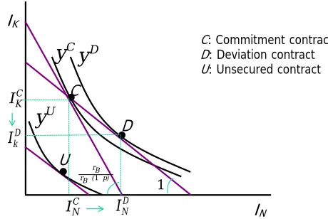
C: Commitment contract

D: Deviation contract

U: Unsecured contract IK

IN

D k

I

C K I

D

C N I

p)β ( B r

B r

− − −

1

1

−

C

y

D

y

U

y

D N

[image:11.612.113.343.463.617.2]

I

Figure 1: Contractible and non-contractible investment. Points C, D, and U represent the optimal input combination and the production level under the commitment, the deviation and the unsecured contract, respectively. PointD is not an equilibrium contract, since the bank does not break even.

However, pointD in Figure 1 is not an equilibrium. Because of the decreased investment in capital

break even, at the contracting stage the bank will be willing to sign only an unsecured contract with all

the repayment obligations paid for in the good state. Setting the collateral equal to zero in the bank

participation constraint (2), solving it for RB and the resource constraint (3) for LB, the objective

function (1) becomes pf(IK, IN)−(IN+IK)rB, which, compared with the benchmark profits (4),

shows the efficiency loss due to the inability of the entrepreneur to pledge collateral. The solution to

the maximization problem is described in Proposition 2.

Proposition 2 When investment is non-contractible, the entrepreneur and the bank sign an unsecured

credit contract. The bank lends LU_B = I_KU +I_NU < LC_B to the entrepreneur, where I_KU and I_NU are

the investment levels solving (30) and (31) in the Appendix, with IU

K < IKC, INU < INC. The bank

gets repaid only in non-defaulting states: RU_B = 1_pLU_BrB. The entrepreneur gets expected profits

ΠU ≡ pf I_KU, I_NU− I_KU +I_NUrB < ΠC. There is an efficiency loss due to the inability to pledge

capital input as collateral.

Point U in Figure 1 is the optimal input combination when investment is non-contractible. The

new isoquant yU lies below yC. While the bank is indifferent between pointsC and U – it gets zero

expected profit either way – the entrepreneur’s profit is strictly lower at B, because the lower debt

capacity implied by the inability to pledge capital inputs as collateral reduces the overall investment

and therefore output. The distance between the isoquants,yC−yU,represents the benefits of collateral.

It follows that, to exploit this benefit, the entrepreneur would rather commit to the investment level

of the secured credit contract (point C). Notice also that at U the actual price of the two inputs is

the same and equal torB (as in pointD), which implies the same level of capital and labor.15

In Proposition 2, we posit that only the unsecured contract (point U) can be an equilibrium

outcome. Both the commitment (point C) and any partially secured contract (any point between C

and U) are time inconsistent since the entrepreneur retains the incentive to alter the input mix in

favor of labor. To get the intuition, consider the relation between the ex ante input price ratio and the

ex post one. As long as these two relative prices are different, there will be an incentive to change the

input combination, no matter how much of the loan has been secured. Consider first the fully secured

contract (pointC in Figure 1). The ex ante input price ratio is rB/[rB−(1−p)β]>1, while the ex

post one isrB/rB= 1. It follows that, once the loan has been granted, labor is actually less expensive

(and capital more expensive), thus inducing the entrepreneur to increase the reliance on labor and

lower that on capital. The same reasoning applies to any partially secured bank loan (i.e., to any

contract where 0 < γ < 1). In this case, the ex ante input price ratio will be rB/[rB−(1−p)γβ],

15

whereγ <1, while the ex post one is 1. Since the ex ante price ratio is still greater than the ex post

one, again labor becomes cheaper ex post, with an ex post incentive to alter the input combination.

3

The commitment role of trade credit

So far we have shown that when the project needs two inputs and the investment in the pledgeable

one is non-contractible, any secured entrepreneur-bank contract (fully or partially) has a problem of

input substitution, which causes losses to the bank. The unsecured loan eliminates this problem but

also the benefits of collateral.

In this section, we introduce the supplier of the pledgeable input as a second financier. By observing

the input transaction, he has a natural information advantage, which the entrepreneur can use to

restore his ability to pledge the capital input as a collateral to the bank. In particular, the entrepreneur

can sign a partially secured credit contract with the supplier. Observing the input transaction and

having a stake in the default state, the supplier guarantees that the input investment is carried out

as contracted. This induces the bank to accept a partially secured credit contract as well, mitigating

the efficiency loss due to the lack of commitment.16

While supplier financing restores the benefits of secured lending, this comes at a cost since trade

credit is assumed to be more expensive than bank credit (rS > rB). To avoid the uninteresting case

in which the cost of trade credit is larger than its benefit, we introduce Assumption 1.

Assumption 1 rB

p ≥

1−γ_prS+

γ p

rB, ∀γ ∈[0,1].

The left-hand side of Assumption 1 represents the financing cost of the pledgeable input when

the entrepreneur does not take trade credit and thus only has access to unsecured bank financing.

The right-hand side is the financing cost when the entrepreneur takes trade credit and also has access

to secured bank credit. When Assumption 1 holds, the cost of finance under the unsecured bank

contract is no less than under any mix of secured trade and bank credit. Thus, taking trade credit

is beneficial to the entrepreneur. The cost on the right-hand side of the expression in Assumption 1

is a weighted average of the fund-raising costs of the bank (rB) and supplier (rS) with weights that

depend on the share of inputs pledged as collateral (γ goes to the bank and 1−γ to the supplier)

and on the probability of default. When default is very likely and the bank liquidates most of the

entrepreneur’s inputs (γ close to 1), having access to a secured bank loan through trade credit is

enormously beneficial, since it reduces the overall cost of financing the inputs. In the extreme case in

16

which γ = 0, the right-hand side of Assumption 1 reaches its upper bound, rS. In this case, it can

still be optimal to take trade credit if rB

p ≥rS. This condition only depends on the model’s parameter

values and turns out to be a sufficient condition for Assumption 1 to be satisfied.

To find the optimal entrepreneur-bank-supplier contract, we proceed in three steps. First, we find

the contract for a genericγ. Next, we show that if the amount of trade credit is too small (γ too high),

the entrepreneur could still “cheat” at the expense of the bank. Finally, we derive the entrepreneur’s

profit under deviation and introduce the incentive compatibility condition that ensures that deviation

is unprofitable. This allows us to determine the incentive-compatible γ and to fully characterize the

optimal contract.

When the bank and supplier can both provide external financing, the optimization problem is

given by programme Pγ_:

max LB,LS,RB,RSIK,IN,γ

p[f(IK, IN)−RB−RS], (9)

s.t. pRB+ (1−p)γβIK ≥LBrB, (10)

pRS+ (1−p) (1−γ)βIK ≥LSrS, (11)

LB+LS ≥IN +IK, (12)

RS ≥(1−γ)βIK, (13)

where (9) denotes the entrepreneur’s expected profit, and (10) and (11) are the participation

constraints of the bank and the supplier, respectively. Condition (12) is the resource constraint

when trade credit is also available, while constraint (13) requires repayments to the supplier be

non-decreasing in revenues.17 Competition among banks and among suppliers implies that (10) and (11)

are binding. In order to minimize the reliance on costly trade credit, the entrepreneur would let the

supplier act only as a liquidator, pledging him the minimum collateral that guarantees commitment,

and setting the repayment in the good stateRS equal to zero. However, this implies that returns be

decreasing in revenues, violating constraint (13). Thus,RSmust be set at the minimum level satisfying

constraint (13), which is then binding. In turn this implies that the supplier gets a flat contract.

Proposition 3 describes the solution to programmePγ_.

Proposition 3 The entrepreneur-bank-supplier contract has investment I_K∗ (γ), I_L∗(γ), solving (32) and (33) in the Appendix, and displays the following properties:

17

a. The supplier gets a secured contract with flat repayments across states: an amount L∗_S(γ) =

1

rS (1−γ)βI

∗

K(γ) is lent in exchange for the right to a share 1−γ of the collateral value of

the unused inputs βI_K∗ (γ) in the default state and a repayment R∗_S(γ) = (1−γ)βI_K∗ (γ) in the

good state; the share of inputs bought on account L∗S(γ)

I∗

K(γ) is decreasing inγ.

b. The bank gets a secured contract with increasing repayments: an amount L∗_B(γ) = I_N∗ (γ) +

h

1− 1

rS (1−γ)β

i

I_K∗ (γ) is lent in exchange for the right to a share γ of the collateral

value of the unused inputs βI_K∗ (γ) in the default state and a repayment R_B∗ (γ) =

1

p[L

∗

B(γ)rB−(1−p) (1−γ)βI

∗

K(γ)] > γβI

∗

K(γ) in the good state. L

∗

B(γ) is increasing in

γ.

c. Expected profits are increasing inγ and β and are given by:

Π∗(γ)≡pf(I_K∗ (γ), I_N∗ (γ))−(I_K∗ (γ) +I_N∗ (γ))rB+

rB

rS

(1−γ) + (γ−p)

βI_K∗ (γ). (14)

d. Asset tangibility IK∗(γ)

I∗

N(γ) is increasing in γ.

In Proposition 3, we derive the properties of the optimal contract for a genericγ. The parameterγ

is the fraction of collateral that goes to the bank and is crucial in our story because it affects both the

entrepreneur’s profit and his incentive to deviate. Since bank credit is cheaper than trade credit, the

higher theγ, the higher the reliance on bank credit, and the higher the entrepreneur’s profit (see point

c of Proposition 3). Thus the entrepreneur would like to setγ as high as possible. However, the higher

theγ,the higher his incentive to deviate from the ex ante contract. The reason is the following. When

the entrepreneur decides to deviate, both the bank and the supplier’s low state return are jeopardized.

However, unlike the bank, prior to the contract execution the supplier observes the change in capital

input provision and refuses to sell the inputs on credit, thus implying a lower total loan and the scaling

down of production by the entrepreneur. The entrepreneur faces therefore a trade-off when deviating:

on one side, the increase in production due to a change in the input mix, and on the other side the

fall in production because of the forgone trade credit. It turns out that, by lowering γ, the bank can

make the fall in production larger, thus affecting the trade-off and the entrepreneur’s incentives to

deviate. The issue is then to determine the maximum γ that prevents deviation (i.e., the value of

γ that makes the entrepreneur indifferent between a mix of secured bank and trade credit and the

deviation contract with forgone trade credit). To this aim, we define the profit from deviation and

Definition 1 Define the entrepreneur’s expected profit after deviating from the contract specified in Proposition 3 as:

ΠF(γ)≡pf I_KF, L∗_B(γ)−I_KF−R∗_B(γ), (15)

where I_KF (L∗_B(γ)) is the level of capital chosen under deviation and satisfying programme PF in the

Appendix.

Given all profitable deviations, the optimal entrepreneur-bank-supplier contract that is incentive

compatible requires that deviation be less profitable than honoring the ex ante efficient contract. This

is ensured by the following incentive compatibility constraint:

ΠF(γ)−Π∗(γ)≤0. (16)

Solving programme Pγ _{under constraint (16) leads to Proposition 4.}

Proposition 4 Under mild conditions, the entrepreneur-bank-supplier contract that prevents

deviation has 0 ≤ γ ≤ γ∗, where γ∗ satisfies condition (16) with equality. Since the entrepreneur’s

expected profitΠ∗(γ)is increasing inγ,the entrepreneur will offer the contract with the highest possible

γ, i.e., γ =γ∗.

In Proposition 4, we identify the optimal share of collateral going to the bank as the upper bound of

the set of collateral shares that are incentive-compatible for the entrepreneur. Usingγ∗ in Proposition

3, we fully characterize the optimal three-party contract. Trade credit is used as a commitment device

and its amount is the lowest possible that makes commitment credible to the bank.

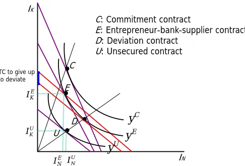
Point E in Figure 2 depicts the input combination and the level of output corresponding to the

entrepreneur-bank-supplier contract implied by Proposition 4. To see why this contract is

incentive-compatible, suppose that initially the entrepreneur signs the three-party contract (pointE) and then

decides to deviate. Upon observing the entrepreneur altering the input mix, the supplier refuses to sell

inputs on credit. This implies a decline in external financing, with a subsequent decline in the scale

of production that makes deviation costly to the entrepreneur. By construction of the

entrepreneur-bank-supplier contract, this decline is such that the entrepreneur is indifferent between sticking to the

original contract and deviating. Graphically, the new optimum under deviation is at pointD, which

lies on the same isoquant as pointE and thus involves the same level of output. The vertical distance

between the isocost lines intersecting pointE and tangent to point D represents the amount of trade

credit the entrepreneur has to renounce to make the contract incentive-compatible. This guarantees

.

.

D E

C: Commitment contract

E: Entrepreneur-bank-supplier contract D: Deviation contract

U: Unsecured contract

IN

IK

TC to give up to deviate

C

.

.

U

C

y

E

y

U

y

E K

I

U K

I

E N

[image:17.612.158.401.81.246.2]

I IUN

Figure 2: The commitment role of trade credit. Points C, E, andU represent the optimal input combination and the production level under the commitment, the entrepreneur-bank-supplier and the unsecured contract, respectively. PointD represents the production level if the entrepreneur deviates from the entrepreneur-bank-supplier contract. PointsD andE lie on the same isoquant.

This discussion implies that whether deviating from the original contract is profitable or not

depends on the amount of trade credit the entrepreneur is getting under the original contract, which

corresponds to the amount he has to forgo in case of deviation. It follows that the bank can always

prevent deviation by reducing its supply of financing (i.e., by reducingγ). By doing so, the bank forces

the entrepreneur to give up a larger amount of trade credit when deviating. This reduces production

so much as to offset the benefit of deviation. The commitment effect of trade credit rests upon two

features of the supplier’s contract. First, the supplier provides a share of the capital input on credit.

Second, the supplier has the right to a share of its collateral value in case of default. Both conditions

have to be satisfied for the entrepreneur to have no incentive to alter the input mix ex post.

Point E lies between point C (commitment contract) and point U (unsecured contract) in Figure

2. The three-party contract does not allow the entrepreneur to achieve pointC since the cheaper bank

credit is partially replaced by the more expensive trade credit. However, it generates larger profit than

the unsecured bank contract. By signaling that the bank loan will be used to purchase the inputs as

specified, trade credit facilitates access to secured bank financing.

Notice that the guarantee implicitly offered in our model by the supplier shares some similarities

with a standby letter of credit. This letter is issued by a financial institution on behalf of the buyer

of some goods to guarantee that the seller will be paid on time and for the correct amount. It works

as a credit-enhancement device and facilitates trade. In our story, the supplier also works as a credit

enhancement device by guaranteeing that there is enough collateral to repay the bank in case of

default, and fosters secured bank lending. Thus, while with a letter of credit it is the bank that

a guarantee to the bank (still on behalf of the buyer). However, besides this similarity, there is an

important difference between a letter of credit and the implicit guarantee offered by the supplier in our

story. Indeed, while a letter of credit brings credit risk to the underwriting financial institution, which

becomes liable in case of buyer insolvency, the supplier in our model does not bear any additional

credit risk and eliminates any risk that the bank will not be fully repaid in default.

3.1 Testable predictions

The discussion above allows us to derive testable predictions on the relation between optimal financial

contracts and the characteristics of the assets invested into the project. Since trade credit allows

entrepreneurs to access secured bank financing, there is a positive relation between the joint use of

trade/secured bank credit and the degree of asset pledgeability. Point E in Figure 2 has indeed

an input combination more intensive in pledgeable assets than point U. Related empirical literature

classifies balance-sheet data on assets into tangibles (with high collateral value as plant, property and

equipment) and intangibles (with low collateral value as patents, goodwill and trademarks). If we use

tangibility as an empirical proxy for the degree of asset pledgeability, we obtain Prediction 1.

Prediction 1. Entrepreneurs are more likely to finance investments intensive in tangible assets with both secured bank and trade credit than with unsecured bank credit only.

The collateral value of an input also depends on its liquidation or scrap value β (i.e., its

second-hand market value, also called degree of input redeployability). While the entrepreneur’s profits

under the three-party contract are increasing in input liquidation value, as shown in Proposition 3,

profits under the unsecured contract do not depend on β, because under such a contract there is no

collateral pledging. Thus the benefits of trade credit (i.e., the difference between the profits under

the commitment and under the unsecured contract) are larger when the input liquidation value is

larger. To some extent, the input liquidation value reflects industry characteristics. For example,

standardized goods are likely to have greater scrap value than differentiated products or services. We

can thus state Prediction 2.

Prediction 2. Secured bank and trade credit are more likely to be used by entrepreneurs buying standardized inputs than by entrepreneurs buying differentiated inputs or services.

The reliance on trade credit also depends on the degree of substitutability between inputs. The

commitment problem arises because the entrepreneur can change the input combination after the loan

has been granted. For trade credit to play a role as a commitment device, inputs need to be at least

partial substitutes. With a higher degree of substitutability between inputs, the commitment problem

proportions, there is no extra-profit to be gained by changing the input combination. Since there is

no incentive to deviate, the entrepreneur can access secured bank financing with no need to use trade

credit. Thus, we obtain Prediction 3.

Prediction 3. Secured bank and trade credit are more likely to be used by entrepreneurs with technologies that have input substitutability than by entrepreneurs with technologies that have inputs

used in fixed proportions.

3.2 A numerical example

In this section, we consider a numerical example to illustrate how trade credit can improve on bank

financing when the entrepreneur is unable to commit to the investment level set at the contracting

stage with the bank. We use the following generic parameter values consistent with Assumption 1:

Y ∈ {0, y},withy=AI_KaI_Lb,whereA= 20, p=.5;a=b=.4;w=ρ= 1;rB = 1;rS = 1.05;β = 0.7.

Commitment contract. If the entrepreneur can commit to the investment level set at the contracting stage with the bank, it relies only on bank credit. Under our parameter assumptions, the

optimal contract, defined in Proposition 1., implies an investment in capital I_KC = 3,728 and labor

I_LC = 2,424. Even if the selling price of the two inputs is the same (w = ρ = 1), the actual input

price ratio (rB/[rB−(1−p)β]) is roughly equal to 1.54. With a ratio greater than one, capital is

relatively less expensive than labor (because of the collateral pledged in the bad state), which explains

why capital investment is larger than labor investment. Input purchase is fully financed by secured

bank financing for an amount LC

B = 6,152. The bank gets the repayment RCB = 9,695 in the good

state and the collateral value of capital inputs C = βI_KC = 2,610, in the bad state. Production is

yC = 6,059 and profits are ΠC = 1,212.

Deviation contract. Suppose now that the entrepreneur cannot commit to the investment level set at the contracting stage. The bank provides the loan of the commitment contract LC

B = 6,152,

expecting returns RC_B = 9,695 andC =βI_KC = 2,610,in the good and bad state, respectively. Upon

being granted credit, the entrepreneur has an incentive to re-optimize and choose a different input

mix. While the entrepreneur will make sure to meet the bank good-state repayment obligation, he is

not concerned with repaying the bank in the bad state. This implies that the entrepreneur solves a

maximization problem where no collateral is pledged. Therefore, the actual input price ratio is now

equal to one, implying an equal amount of capital and laborI_KD =I_LD = 3,076. With the input price

ratio under deviation (called ex post) lower than the ratio under the commitment contract (called ex

why the entrepreneur wants to deviate and reduce the investment in capital below the commitment

level. Under the new input choice, both production and profits increase to yD = 6,172 > yC and

ΠD = 1,324 >ΠC, respectively. While the entrepreneur is clearly better off, the bank is worse off.

Because of the lower investment in capital input, the bank return in the bad state (i.e., the capital

input liquidation value) is strictly lower than the contracted one: βI_KD = 2,153<2,610 =βI_KC. Thus,

the bank no longer breaks even and the deviation contract is not an equilibrium contract.

Unsecured contract. Anticipating the entrepreneur’s deviation, the bank offers the fully unsecured contract described in Proposition 2. This contract implies a smaller loan amount than

in the commitment contract LU_B= 2,048< LC_B = 6,152, due to the entrepreneur’s inability to pledge

the collateral as partial repayment of the loan. The bank gets a repayment only in the good state

equal to RU_B = 4,096. Since the contract is unsecured, there is no incentive to deviate. Moreover,

an equal amount of capital and labor is invested, IU

K = ILU = 1,024. Due to the lower loan size,

production and profits are strictly lower than in the commitment contract: yU = 2,560< yC = 6,059

and ΠU = 512< ΠC = 1,212. Thus, the unsecured contract eliminates the entrepreneur’s incentive

to deviate but also the benefits of the collateral. The entrepreneur would be better off if he could

credibly commit to the input combination agreed in the commitment contract.

Entrepreneur-bank-supplier contract. To credibly commit to the input mix specified in the commitment contract, the entrepreneur takes trade credit. Since trade credit is more expensive than

bank credit, it is optimal to take the minimum amount of trade credit that stops deviation and rely

for the rest on the cheaper bank credit. Trade credit is L∗_S = 374 and it allows the entrepreneur to

access an amount of secured bank financing equal to L∗_B = 5,654. Both financiers get a repayment

in the good state: R_B∗ = 9,151, R∗_S = 392. In the bad state, the collateral value of capital inputs

is shared, with a fraction 1−γ∗ = 0.15 going to the supplier and γ∗ = 0.85 to the bank. With

trade and bank credit together, the entrepreneur gets a total loan strictly larger than the one

received under the unsecured contract and close to the one under the commitment contract, i.e.,

LU_B = 2,048<(L∗_B+L∗_S) = 6,028< LC_B = 6,152, with trade credit being only 6% of the total loan.

This allows the entrepreneur to invest I_K∗ = 3,641 andI_L∗ = 2,386 in capital and labor, respectively,

obtaining slightly lower profits than in the commitment contract, but strictly larger profits than in

4

Entrepreneur-supplier collusion

In Section 3, we argued that trade credit enables the entrepreneur to overcome the problem of

commitment with the bank. This is because the supplier will always refuse to extend credit upon

observing the entrepreneur’s deviation, as he will fail to break even on the new input combination.

This might not be true anymore if the contract between the entrepreneur and the supplier were

renegotiated to allow the supplier to at least break even. In this section, we extend the model to allow

for collusive agreement between the entrepreneur and the supplier.

Suppose that the entrepreneur, the bank, and the supplier have agreed on the contract terms

described in Proposition 3, with γ =γ∗. Once the loan from the bank is obtained, the entrepreneur

may then seek an agreement with the supplier to alter the input mix at the expense of the bank (i.e.,

to reduce the investment in capital and increase that in labor). If the supplier is to accept, they must

renegotiate the contract terms (i.e., loan size and repayments), so as to enable the supplier to at least

break even:18

pRS+ (1−p) (1−γ)βIK ≥LS(γ)rS. (17)

If agreed, the new arrangement allows an increase in overall profits at the expense of the bank. This

allows us to define the gross collusion rent and describe its properties in Proposition 5.19

Definition 2 Define ΠCOL(γ) as the profit from collusion for a generic γ solving programme PCOL

in the Appendix andΠCOL(γ)−Π∗(γ) as the gross collusion rent, where Π∗(γ) is the profit from the

entrepreneur-bank-supplier contract as defined in Proposition 3 for a generic γ.

Proposition 5 The gross collusion rent ΠCOL(γ)−Π∗(γ) is increasing in γ and is zero iff γ = 0.

Thus, any entrepreneur-bank-supplier contract is vulnerable to collusion between the entrepreneur and

the supplier at the expense of the bank.

In Proposition 5, we posit that a collusive agreement to alter the input combination ex post is

always profitable for the entrepreneur and the supplier. Thus, the entrepreneur-bank-supplier contract

is not collusion-proof. The only way for the bank to stop other parties from colluding is to offer an

unsecured contract (γ = 0). However, reaching a collusive agreement may be costly. This cost may be

due to the time and effort spent in writing and enforcing the side contract. It may also be the effect

18_{An alternative collusive agreement would keep the loan size fixed (L}∗

S(γ

∗

)) and renegotiate only the repayments schedule. However, while this would not alter the qualitative properties of the collusion-proof contract, there is no real reason to impose this constraint on the renegotiation. Moreover, renegotiating all the contract terms is profit-maximizing, as it gives the entrepreneur the possibility of reducing its reliance on costly trade credit.

19_{For simplicity we assume that any collusive rent is seized by the entrepreneur. This is without loss of generality, as}

of reputational concerns.20 To capture this cost, define α ∈ [0,1] as the fraction of the profit from

collusion that is lost in reaching such an agreement and [(1−α) ΠCOL(γ)−Π∗(γ)] as the net rent

from collusion. This formulation enables us to find an interior γ that stops parties from colluding.

In particular, for a sufficiently high α, the bank can always prevent collusion by focusing on contract

offers that guarantee a non-positive collusion rent, i.e., those that satisfy the following constraint:

(1−α) ΠCOL(γ)−Π∗(γ)≤0. (18)

Is the entrepreneur-bank-supplier contract collusion-proof when we measure the collusion rent net

of bargaining costs? More specifically, at γ =γ∗ (the value of γ that ensures no unilateral incentive

to deviate), is constraint (18) satisfied? The answer depends on the cost of collusion,α. Let us define

α∗(γ∗) as the value of α at which the collusion-proof constraint (18) is satisfied with equality when

γ =γ∗. Whenα≥α∗(γ∗), the value ofγ that solves (18) is greater thanγ∗,so that the

entrepreneur-bank-supplier contract can also accommodate collusion. Whenα < α∗(γ∗), the value ofγ that solves

(18) is less than γ∗ and the entrepreneur-bank-supplier contract is open to collusion. This amounts

to saying that the value of γ that accommodates both unilateral deviation and collusion has to solve

the following global collusion proofness constraint:

max

(1−α) ΠCOL(γ),ΠF(γ) −Π∗(γ)≤0. (19)

This allows us to state the result in Proposition 6 and then to derive Corollary 1.

Proposition 6 The collusion-proof entrepreneur-bank-supplier contract has γ = ˆγ(α) ≤ γ∗, where ˆ

γ(α) satisfies condition (19) with equality. The properties of this contract are those described in

Proposition 3, with γ = ˆγ(α).

Proposition 6 implies that the properties of the collusion-proof contract, and thus the benefits of

using trade credit, depend on the cost of collusion. Three scenarios can arise. First, collusion can be

so costly that it is never profitable: α(γ∗)≤α≤1. The rent from collusion is lower than the rent from

deviation, so that the global collusion-proof condition (19) coincides with the incentive-compatibility

condition (16). This corresponds to the case already analyzed in Section 3: The entrepreneur buys

commitment from the supplier through trade credit and takes a partially secured loan from the bank.

The share of capital inputs bought on account (through trade credit) isβ(1−γ∗) and the share paid

in cash (through bank credit) isβγ∗. Both shares are independent of α. The equilibrium is at point

E in Figure 2 and the input combination is capital intensive.

20

Second, collusion may be costly, but profitable: 0 < α < α(γ∗). The rent from collusion is

greater than from deviation, so that the global collusion-proofness condition (19) coincides with the

collusion proofness condition (18). The lower the cost of collusion, the larger the amount of trade

credit necessary to make the contract collusion-proof, and the lesser the bank’s participation in the

venture. It follows that the lower the cost of collusion, the larger the share of inputs bought on account

through trade credit, and the lower the one bought through bank credit. The properties of the optimal

contract are those described in Proposition 3, withγ = ˆγ(α). The equilibrium point is located between

pointsE and U in Figure 2, the exact position depending on the cost of collusion. The lower the cost,

the further the equilibrium shifts from point E to pointU, with the input combination becoming less

capital-intensive.

Lastly, collusion may be costless (α = 0). The entrepreneur and the supplier can grab the entire

surplus from their agreement. In this case, the only contract that enables the bank to break even is

the unsecured one (pointU in Figure 2). Since the bank does not have a stake in the bad state return

any longer, the bank is reimbursed only in the good state. This arrangement removes any incentive

to collude.

From Proposition 6 and the above discussion, we can derive Corollary 1.

Corollary 1 Under the collusion-proof contract, the share of inputs bought by the entrepreneur on

credit is decreasing in the cost of collusionα, while the share of inputs paid for in cash, asset tangibility,

and expected profits are increasing in α.

5

Relationship lending and trade credit in a multi-period setting

So far we have shown that when the investment in the capital input is not contractible, any secured

bank contract is time-inconsistent and trade credit can be used to solve the problem and give the

entrepreneur access to secured bank financing. These results depend on the information advantage of

the supplier vis-`a-vis the bank: The supplier, as a provider of the input, knows the investment level

in capital, the bank does not. This argument could suggest that our conclusions strictly depend on

the static nature of the credit relations. In a dynamic setting, the bank could exploit the repeated

interaction to set up a long-term relationship, where information about the past investment level

can be collected and used to determine future contract terms, possibly incorporating a penalty for

misbehavior. Anticipating a future punishment in case of deviation, the entrepreneur would have an

incentive to abide by the contract and there might be no need to use trade credit. The threat of a

We formally study this possibility by extending the static baseline model to a multi-period setting,

similar in spirit to Boot and Thakor (1994), where an intertemporal price-adjustment mechanism

is used to reduce efficiency losses from using collateral. In Section 5.1, we assume the information

collected by the bank to fully reveal the past investment level (perfect signal). In Section 5.2, we

consider instead the case of a noisy signal. We show that trade credit is still the most efficient way to

solve the commitment problem, provided that the duration of the project is not too long.

5.1 A perfect signal

Structure of the repeated game. Consider an economy where the entrepreneur has to finance the project defined in Section 1. This project has a duration of t = T > 1, that is, it can be repeated

for a finite number of periods, T. The entrepreneur enters a long-lasting lending relation with one

bank and signs a long-term contract that specifies the contract terms for anyt= 1, ..., T,contingent

on some information about the past investment level. We denote this financing scheme relationship

lending, because the bank gathers proprietary information through the repeated interaction with the

borrower and uses it to set future contract terms.21

In each period, the entrepreneur faces the commitment problem described in Section 2. He

can invest the amount of inputs specified in the commitment contract (cooperation), gaining the

commitment profits ΠC defined in Proposition 1. Alternatively, he can choose a different input mix

(deviation) and gain the deviation profits ΠD (equation 8). At the end of each period, the bank obtains

a signal revealing with certainty the chosen investment level, which can be used to set the following

period’s contract terms.22

To derive the sequence of profits conditional on each possible decision and on the signal received

by the bank, let us start from the last period. At t=T, the parties cannot agree on a commitment

contract as the entrepreneur surely deviates. Thus, the only contract the parties will agree on is an

unsecured contract, whose price depends on the signal received by the bank. In particular, if the

information reveals cooperation, they agree on the unsecured contract derived in Proposition 2 and

the entrepreneur gets the resulting profits, ΠU. If the information reveals deviation, the bank penalizes

the entrepreneur by charging a higher interest rate (punishment contract) and the entrepreneur gets

profits ΠP <ΠU.23 Profits ΠP are defined later.

21

See Boot (2000) for a review of the literature on relationship lending.

22_{Assuming that the entrepreneur can collect this information also in the static setting would not alter any of our}

results, since the information can only be used with one period lag.

23_{In the last period of the game, the contracts need to be contingent on the information revealed. If not, we end up}

At any timet < T, instead, the parties agree on a commitment contract if the signal collected by

the bank revealed commitment by the entrepreneur in the previous period, or else on a punishment

contract for only one period if the signal revealed deviation, followed by a commitment contract in

any successive period, until a deviation signal triggers a punishment contract again.

Cooperation as an optimal strategy. Given the strategy defined above, we have a sequence of

T entrepreneur’s decisions with associated profits. For simplicity, we assume that the discount factor

is zero.24 In Proposition 7, we posit the condition under which cooperation in all periods weakly

dominates deviation in any one period.

Proposition 7 Under the strategy defined above, cooperation weakly dominates deviation iff:

ΠD−ΠC ≤ΠU−ΠP. (20)

Condition (20) indicates that in any T-period model, the incentive constraint that guarantees

cooperation reduces to a comparison between the one-period deviation benefit (left-hand side) and the

last period deviation cost (right-hand side). Therefore, the entrepreneur will cooperate if the benefit

from deviation is lower than the cost. This crucially depends on the punishment profits ΠP,and thus

on the penalty P the entrepreneur has to pay when deviation is detected by the bank.

The next step is to derive the minimum penalty that prevents deviation (i.e., satisfies condition

(20) with equality). Suppose that in a generic period the signal reveals that the entrepreneur has

deviated. This triggers the punishment contract in the following period. This contract is unsecured

as the one defined in Section 3, but with a higher interest rater0_B that incorporates the penaltyP for

deviation. The terms of the punishment contract and the corresponding investment levels are thus set

to solve the following optimization programme (PP):

max IK,IN,LB,RB,P

p[f(IK, IN)−RB]

s.t. pRB =LBrB0 (21)

LB=IK+IN

under the additional no-deviation condition (20). The constraints above have the usual meaning, the

only novelty being thepunishment interest rater_B0 ≡rB+_LP

B in the individual rationality constraint

(21). This interest rate is made of two components: the market interest rate,rB,plus an extra variable

cost calculated as a fraction of the penaltyP the entrepreneur has to pay upon deviation on the total

loan received, LB.

24

Solving programmePP, we obtain the entrepreneur’s profits under the punishment contract as:25

ΠP ≡pf I_KP, I_NP

−LP_B

rB+

P LP

B

<ΠU. (22)

The analysis above posits that under a sufficiently high punishment, relationship lending eliminates

the entrepreneur’s incentive to deviate and provides a viable solution to the commitment problem of

secured lending.

Relationship lending versus trade credit. We now compare two alternative ways to solve the commitment problem of secured financing. On the one hand, we have relationship lending with a

long-term contract that specifies a sequence of credit amounts and repayment obligations contingent

on the borrower’s investment history. On the other hand, there is a sequence of single-period trade and

bank credit contracts, independent of past project investment and with potentially different suppliers

and lenders at each point in time. For brevity, we use the termtrade credit to identify this three-party

contract. If the entrepreneur uses relationship lending, he signs the long-term bank contract that

guarantees cooperation in all periods, getting the commitment profits ΠC derived in Proposition 1 for

T −1 periods and the profits from the unsecured contract ΠU in the last period. The total profits

under relationship lending are thus (T −1)ΠC+ ΠU.If he uses trade credit, he signs the three-party

contract defined in Proposition 3 repeatedly for any of the T periods and gets the expected profits

Π(γ∗), renamed here ΠT C in each period. Thus, the total profits under trade credit areTΠT C.

It follows that relationship lending is preferred to trade credit if the following condition is satisfied:

(T−1)ΠC + ΠU ≥TΠT C. (23)

When T = 1, condition (23) is never satisfied since ΠU <ΠT C. This case coincides with the baseline

model: when the project lasts for one period, the commitment problem can only be solved by using

trade credit. When the game is repeated, cooperation can be achieved and the entrepreneur can gain

the commitment profits ΠC forT−1 periods at the cost of getting lower profits ΠU in the last period

for his inability to credibly commit. With increasing iterations, the weight of ΠU reduces while that

of ΠC increases, so that at some point it becomes more profitable to enter a long-term relationship

with the bank rather than relying on trade credit. This discussion is summarized in Proposition 8.

Proposition 8 Under perfect signal, there is critical duration of the project:

T∗= 1 + Π

T C_−ΠU

ΠC_−ΠT C >1, (24)