A novel size independent symplectic analytical singular element for inclined crack terminating at bimaterial interface

A novel size independent symplectic analytical singular element for

inclined crack terminating at bimaterial interface

XF Hua, b_{, QS Shen}a, b_{, JN Wang}c_{, WA Yao}a, b*_{, ST Yang}d

a _{State Key Laboratory of Structural Analysis for Industrial Equipment, Dalian University of Technology,} Dalian 116024, China

b _{International Research Center for Computational Mechanics}

c_{Beijing Institute of Structure and Environment Engineering, Beijing, China}

d _{Department of Civil and Environmental Engineering, the University of Strathclyde, Glasgow, G1 1XJ,} United Kingdom

*_{Corresponding author: [email protected]}

Abstract: Cracks often exist in composite structures, especially at the interface of two different materials. These cracks can significantly affect the load bearing capacity of the structure and lead to

premature failure of the structure. In this paper, a novel element for modeling the singular stress state

around the inclined interface crack which terminates at the interface is developed. This new singular

element is derived based on the explicit form of the high order eigen solution which is, for the first time,

determined by using a symplectic approach. The developed singular element is then applied in finite

element analysis and the stress intensity factors (SIFs) for a number of crack configurations are derived.

It has been concluded that composites with complex geometric configurations of inclined interface

cracks can be accurately simulated by the developed method, according to comparison of the results

against benchmarks. It has been found that the stiffness matrix of the proposed singular element is

independent on the element size and the SIFs of the crack can be solved directly without any

Keywords: Composites, inclined interface crack, high order eigen solution, singular element, stress intensity factors

Nomenclature

( )i _{, 1,2,3,...}

a i eigen expanding coefficients

a vector of the eigen expanding coefficients

, , ,

A B C D coefficients of the general expression of eigenvector

A diagonal matrix of which the elements are composed of eigenvalues

B B A ( ln )

C matrix of the general expression of eigenvector

d vector of nodal displacements

D vector of the coefficients , , ,A B C D

,

E  Young’s modulus and Poisson’s ratio

F matrix generated from substituting eigenvector into the boundary condition

G shearing modulus

G second part of the characteristic equation of eigenvector

H Hamiltonian operator matrix

I identity matrix

J unit symplectic matrix

, , ,

k k k k    k p a b c d, , , , , coefficients in the relationship between the eigenvectors of the

region #1 and the region #2

, , ,

k k k k      ka b c d   , , , , coefficients in the relationship between the eigenvectors of the

region #3 and the region #2 ,

I II

K K mode I and mode II stress intensity factors

K stiffness matrix of the SASE

L characteristic length

M , N positive integers

p_, q _{vectors of the configuration variables and the dual variables}

*

p , _q* _{vectors of trail functions of the configuration variables and the dual variables}

( , )r  polar coordinate system

R generalized stiffness matrix of the SASE

, ,

r r

S S S  generalized stress components

*_{, ,}* *

r r

S S S_{ } trial functions of the generalized stress components u

T matrix of which the elements are values of eigenvector on the export nodes ,

r

u u_ displacement components

*_, * r

u u trail functions of the displacement components

,  the Dundurs parameters

 oscillation index (bimaterial constant)

, ,

r  r

   strain components

, ,

r  r

   stress components

 generalized coordinate

1, , ,2 3 4

    ₁    , 2   , 30, 4   

 _eigenvalue

ψ _eigenvector

, , , ,

u v r r 

     variables separated from displacement and stress variables

Φ, Θ matrices of which the elements are composed of eigenvectors

Π deformation energy of the SASE

 _{radius of the SASE}

 =E E₂ / ₁, the ratio of the Young’s moduli of the two materials

1.Introduction

Composite materials are widely used in various engineering sectors due to their optimal properties

compared with a single material. However, it is almost inevitable for the composite materials to possess

cracks or defects, especially at the interfaces between two joining materials, under fabrication process,

environmental degradation, applied loads, etc. The cracks can propagate, accumulate and significantly

reduce the load bearing capacity of the structure in terms of fracture failure. Perhaps due to the

mathematical complexities in formulating the interface crack, most of the existing studies in literature

focused on a special case where the crack is along the interface of the two materials [1, 2, 3, 4, 5, 6, 7, 8, 9]_.

However, a more general and challenging case in which the crack lies in an angle with the interface and

terminates at the interface should also be sufficiently addressed. Since the crack can be treated as being

inclined from an interface crack, it is named inclined interface crack in this paper.

Stress Intensity Factors (SIFs) and Energy Release Rates (ERRs) have been widely employed for

quantifying the stress singularity around the crack. Cook studied the stress state around the crack

terminating at the bimaterial interface, and proposed a fracture criterion for crack initiation [10]_{. Lin and} Mar considered the case in which the crack was perpendicular to the material interface. They developed

a hybrid element to calculate the SIFs and the ERRs[11]_{. Chen derived a general expression for the} singular stress field around the inclined interface crack, and employed the body force method to

calculate the SIFs[12]_{. In addition, Wang and Per developed a model for solving the SIFs and the T}

stresses around the crack tip[13]_{. Lin and Sung}[14] _{and Poonsawat et al.}[15] _{analyzed the stress singularities} of the inclined interface crack in anisotropic materials. Furthermore, Wijeyewickrema et al. studied the

stress singularities of the crack terminating at the frictional interface of monoclinic bi-material

Finite element (FE) analysis is popular in engineering applications; however, if conventional

elements were used, extensive mesh refinement around the crack tip would have been employed to

ensure the accuracy of simulation [17]_{. Different numerical methods have been developed to study crack} problems in engineering including meshfree method [18, 19, 20, 21, 22]_{, extended finite element method}

(XFEM) [23, 24, 25, 26, 27, 28]_{, extended isogeometric analysis (XIA)} [29, 30, 31]_{. These methods are used to} calculate SIFs or ERRs for crack problems with high solving efficiency. However, only a few numerical

methods can be applied to inclined crack terminating at bimaterial interface. Bouhala et al.[27] _studied the inclined interface crack problem by using XFEM, the stress and displacement enrichment functions

were determined by considering plane elasticity solution based on Airy functions. Natarajan et al.

applied the extended scaled boundary finite element method (xSBFEM) to the inclined interface crack

problem, and both SIFs and T stresses were solved numerically without path independent integral[32]_.

Nasri et al. investigated the behavior of the crack terminating at the zinc/steel bimaterial interface with

different orientations by using the FE software package ABAQUS[33]_.

More recently, cohesive crack model is applied to the modeling of the bimaterial interface cracks.

Adams modeled the crack which was perpendicular to the bimaterial interface and found that the critical

value for crack propagation depended upon the maximum stress of the cohesive crack model, as well as

the Dundures parameters[34]_{. Mehidi et al. investigated the crack normal to the metal/alumina interface} by determining the J integral and the plastic zone at the crack tip using the three-dimensional finite

element methods[35]_{. Muthu et al. developed a new variant of the element-free Galerkin (EFG) method,}

and applied this new method for the inclined bimaterial interface crack problem[36]_{. Chang and Jeng} developed a “Mint” contour integral for the cracks passing through or terminating normally at the

For these existing methods in solving the inclined interface crack, the conventional FE analysis

requires extensive mesh refinement around the crack tip and the solving efficiency is therefore reduced.

XFEM[17] _{employs the asymptotic fields as the enrichment to improve the solving accuracy, however, it} is still not satisfactory because, (1) dense meshes around the crack tip are also required to achieve

acceptable accuracy; (2) the implementation in the XFEM is very complex. The elements isolated by the

crack and the interface should be partitioned into subtriangles for the purpose of integration and the

blending elements are required to connect the crack tip enriched element to the standard elements; (3)

the numerical prediction is sensitive to the numerical integration scheme used for the enriched elements.

In Ref.[27], different integration schemes were used for different types of elements, i.e., a

thirteenth-order Gaussian integration method was used for the subtriangles at the crack tip, a sixth-thirteenth-order Gaussian

integration scheme was used for the subtriangles at the crack surface and a sixteenth-order Gaussian

integration scheme was used for the blending elements. In light of the existing methods in modeling the

inclined interface cracks, it has been found that the description for the displacement and stress fields

around the crack tip is of crucial importance. Although the enrichment terms as well as the standard FE

shape functions are available in XFEM, further improvement is still desirable. Therefore, a combination

of numerical method and analytical solution, which strictly satisfies all the fundamental equations,

compatibility condition and the boundary condition, could bring many advantages. It is in this regard

this paper is presented.

In this study, for the first time, the analytical eigen solution of the complex inclined interface crack

is derived by using the symplectic method. Based on the obtained analytical eigen solution, a new

symplectic analytical singular element (SASE) is developed for numerical simulation. The SIFs are then

calculated directly without any post-processing. It should be noted that the stiffness matrix of the

important role in ensuring accuracy and stability of numerical simulation. The symplectic approach for

elasticity[38, 39] _{has emerged as a useful tool for the analytical study of singularity problems. By using the} symplectic approach, analytical eigen solutions for different crack problems were obtained[40, 41, 42, 43, 44, 45 ]_{. The rich information of displacement and stress fields around crack tip expressed in terms of}

analytical solution could lead to better solving accuracy and efficiency. Based on the existing analytical

eigen solutions, a series of analytical singular elements were developed for the numerical study of

cracks[46]_{, bimaterial interface crack}[40, 47]_{, fatigue crack growth}[48] _{and Dugdale model based cracks}[49, 50]_{. These elements were termed as "singular element" or "enriched element" in the early publications}

[40, 46, 48, 49, 50]. However, considering the methodology used for construction of the element and its

applications, the new developed elements in the recent publications [47, 51, 52, 53] were termed as

Symplectic Analytical Singular Element (SASE). In the future, SASE will be consistently used.

A few examples are worked out to demonstrate the application of the proposed method.

Verification of the results against the benchmarks has indicated that the developed model is very

accurate in capturing the stress state around the inclined interface crack.

2.Fundamental equations

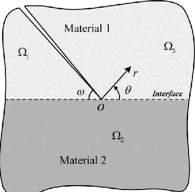
Considering an inclined interface crack terminating at the bimaterial interface as shown in Fig.1,

the origin of the polar coordinate system is located at the crack tip. The crack orientation is denoted by

    where  is an arbitrary angle satisfying   0. For a special case, the problem becomes

a bimaterial interface crack problem[40] _{when 0 or}   _{. The domain is divided into three regions}

by the crack and the material interface as shown in Fig.1. The subscript “i” (i1,2,3) is employed to

represent each region. The Young’s modulus and Poisson’s ratio of the material in the ith region are Ei,

i

sake of convenience, the subscript “i” (i1,2,3) is omitted in the equations hereinafter except where it may cause confusion.

The fundamental equations of this problem under the assumption of plane stress are briefly

presented below. The equilibrium equations neglecting the body force can be specified as follows,

1

0

2 1

0

r r r

r r

r r r

r r r

                  _{  }       _{  }     (1)

where r,  and r are stress components. The relationship between strain and displacement is

specified as follows

1 1 r r r r r u r u u r r

u u u

r r r

              _       _     _{  }  _{ }  (2)

where r,  , r are strain components, while ur and u are displacements along radial and angular

directions respectively. The Hellinger-Reissner (H-R) variational principle of the discussed problem is specified by





1 3 , , , , , , , , , 0 1

2 2 2

, , , , ,

1 δ

1

2 2 1 d d 0

2

i

i

r i i i i i r i

r i r i r i

i

i r i i r i i i r i

i

u u u u u

u

r r r r r

r r E  _{   }                           _  _ _  _{ }   _{       }          _     _  

 

(3)

where 1    , 2   , 30 and 4    . Assuming that the two materials are perfectly

bounded, then the compatibility condition at the material interface can be obtained by

,1 ,2, ,1 ,2, ,1 ,2, ,1 ,2

r r r r

,2 ,3, ,2 ,3, ,2 ,3, ,2 ,3

r r r r

u u u_ u_ _ _ _  _ , at 0 (5)

The traction free boundary condition on the crack surfaces can be expressed as follows

,1 r ,1 0

 

   _{, at }   _{ } (6)

,3 r ,3 0

 

   , at     (7)

Due to the mathematical complexities, the problem described above is difficult to be solved by using

conventional methods. This study employs a novel symplectic approach, by using which the original

problem is transformed into a symplectic eigenvalue problem which is then solved analytically.

3.Symplectic approach

The symplectic approach for elasticity has been widely applied for the analytical study of singularity

problems[38, 39]_{. By using this approach, the governing equation of the original problem is reduced into a}

series of first order differential equations which is then transformed into an eigenvalue problem by the

method of separation of variables. The symplectic approach is employed in this study to solve the eigen

solution of the complex inclined interface crack. By introducing the generalized coordinate

lnr

  (8)

and the generalized stress components

, ,

r r r r

S r S_ r_ S_ r_ (9)

the H-R variational principle expressed in Eq.(3) can be rewritten as





1 3 , , , , , , , , , 0 1

2 2 2

, , , , ,

1 δ

1

2 2 1 d d 0

2

i

i

r i i i r i

r i i r i r i i

i

i r i i r i i i r i

i

u u u u

S S u S u

r

S S S S S

E  _{ }                        _  _ _  _{ }   _  _   _{ }           _     _  

 

(10)

r r

u

S E u  S

 _ 



 

 _  _



  (11)

Substituting Eq.(11) back into Eq.(10), the equivalent H-R variational principle can be further simplified as follows: 1 3 , , , , , , , , , 0 1 2

, 2 2 2

, , ,

δ

1

(1 ) 2(1 ) d d 0

2 2

i

i

r i i i r i

r i i r i r i r i i

i

i i

r i i r i i r i

i

u u u u

S S u S u

u E

u S S

E  _{ }                        _  _ _  _{ }   _  _   _{ }          _  _{     } _   _      _

 

(12)

From Eq.(12), there are four independent variables in the equivalent H-R variational principle, i.e., ur,

u_, Sr and Sr. Making variations of Eq.(12) with respective to these independent variables gives the

symplectic dual equation which is specified by,



 _



Z

HZ ₍₁₃₎

where _{[ , , , ]}T

r r r

u u S S_{ }



Z is the unknown vector of the configuration variables _{[ , ]}T r

u u_



p and the

dual variables _{[ , ]}T

r r

S S



q . Moreover, the Hamiltonian operator matrix H is presented as follows,

2 2 2 1 0 2(1 ) 1 0 1 E E E E E E               _{ }     _       _   _    _{ }   _       _{  }            H (14)

The symplectic dual equation expressed in Eq.(13) can be solved by the method of separation of

variables, let

( , )  e ( )

where  is the symplectic eigenvalue and T

( ) [     u v r r]

ψ is the corresponding symplectic

eigenvector. u, v, r and r are variables which are, respectively, separated from the original

variables ur, u , Sr and Sr. Similarly,  is denoted as the variable separated from S. Substituting

Eq.(15) back into Eq.(13), the original problem is transformed into a symplectic eigenvalue problem,

presented as follows,

( )  ( )

Hψ ψ (16)

The eigenvalues of the Hamiltonian operator matrix H have some particular behavior that if a non-zero

eigenvalue  is an eigenvalue then  must also be an eigenvalue[38]_{. So the non-zero eigenvalues are}

divided into two groups,

(a) _( , ) j _{,j1,2,3,..., Re(}( ) _{) 0 or, Re( }( ) _{) 0 and Im( }( ) _{) 0 (17)}

(b) _( , ) j _{,j1,2,3,...,}( ) _{ }( )a ₍₁₈₎

The corresponding eigenvectors are denoted by _ψ( , )j _{and ψ}( , ) j _{, respectively. The superscript}

1,2,3,...

j is employed to denote the thj eigen solution, it will be ignored where applicable for the

sake of simplicity. We define the symplectic inner product between two arbitrary vectors in the

symplectic space as

1 3

T 1

, i d

i

a b a b

i



 





ψ ψ 



ψ Jψ (19)

where 0

0

 

_ 

 

I J =

I is a unit symplectic matrix for the identity matrix I and the values of 1, 2, 3

and 4 have been defined above. It is proven that if  is a single root, then the symplectic eigenvectors

( , ) j

ψ and _ψ( , ) j _{are mutually adjoint symplectic orthogonal to each other}[38]_{. And if}  _{is a repeated}

among the eigenvectors are normally used to solve the exact solutions[43]_{, it is introduced here just for}

completeness, more detailed discussions can be referred to Ref.[38].

By using the generalized stress components, the compatibility condition at the material interface

expressed in Eqs.(4) and (5) can be rewritten as follows,

,1 ,2, ,1 ,2, ,1 ,2, ,1 ,2

r r r r

u u u_ u_ S_ S_ S_ S_ , at   (20)

,2 ,3, ,2 ,3, ,2 ,3, ,2 ,3

r r r r

u u u_ u_ S_ S_ S_ S_{ , at 0 (21)}

The traction free boundary condition on the crack surfaces can be rewritten as follows,

,1 r ,1 0

S_ S_  _{, at      (22)}

,3 r ,3 0

S_ S_  _{, at   }  (23)

4.Symplectic eigen solution

As formulated, the original problem has been transformed into a symplectic eigenvalue problem, e.g., in

Eq.(16), subjected to compatibility condition and boundary condition. In solving the eigenvalue

problem, the special case with zero eigenvalue and the general case with non-zero eigenvalue should be

considered separately.

4.1.Zero eigenvalue and eigenvector

For zero eigenvalue, the corresponding eigenvector can be obtained by solving

( ) 0 

Hψ (24)

The eigenvectors can be obtained as follows,

(1) _{[cos( ) sin( ) 0 0]} T

ψ , _ψ(2) _{[sin( ) cos( ) 0 0] } T ₍₂₅₎

Obviously, they represent rigid body transitions along horizontal and vertical directions, respectively.

T

(1, ) 1 _{sin( )} 1 _{cos( )} 1 _{sin( ) cos( ) 0}

2 2 2

J _ _{ } _{  }  _{ E } 

 

 

ψ (26)

T

(2, ) 1 _{cos( )} 1 _{sin( )} 1 _{cos( ) sin( ) 0}

2 2 2

J _{ } _{ } _{  }  _{ E } 

 

 

ψ (27)

where _ψ(1, )J _{and ψ}(2, )J _{are the Jordan form eigenvectors corresponding to ψ}(1) _{and ψ}(2)_{, respectively.}

Combining the original eigenvectors and the corresponding Jordan form eigenvectors together, the

Jordan form eigen solutions of the original problem can be determined and presented as follows

(1, )J _ (1, )J _ (1)

Z ψ ψ , _Z(2, )J _ψ(2, )J _ψ(2) ₍₂₈₎

It may be noted that the above Jordan form eigen solutions are concentrated forces acting at the

coordinate origin along horizontal and vertical directions, respectively.

4.2.Non-zero eigenvalue and eigenvector

For non-zero eigenvalue, the general solution of the eigenvector of Eq.(16) for the material in the ith

region can be solved and specified by

i  i i

ψ C D, (i1,2,3) (29)

where the explicit expression of the matrix Ci is given in Eq.(A1) in the Appendix.

T

[ ]

i  Ai Bi Ci Di

D is the vector of the coefficients Ai, Bi, Ci and Di . There are totally 12

coefficients in the eigenvectors for the three regions whilst only four of them are independent. Therefore,

only the coefficients of the region #2 (A2, B2, C2 and D2) are chosen as independent coefficients. The

relationship among the coefficients is determined through the compatibility condition at the material

interface as specified in Eqs.(20) and (21). Substituting the general solution of the eigenvector Eq.(29)

1 2 2 2 2

1 2 2 2 2

1 2 2 2 2

1 2 2 2 2

A a p A a p B a p C a p D B b p A b p B b p C b p D C c p A c p B c p C c p D D d p A d p B d p C d p D

       

       

       

       

   



    



    



 _{   }



(30)

where the expressions of the coefficients k_, k_, k_, k_ (k p a b c d, , , , ) in the above equations are given in Eqs.(A3), (A4) and (A5) in the Appendix. Similarly, substituting Eq.(29) into Eq.(21) the

coefficients of region #3 can also be represented by these of region #2, the relationship is specified by

3 2 2

3 2 2

3 2 2

3 2 2

A a p A a p C B b p B b p D C c p A c p C D d p B d p D

   

   

   

   

 

 



 _{   }



 _{   }



    



(31)

in which the expressions of the coefficients k_, k, k, k (ka b c d   , , , ) are given in Eq.(A6) in the

Appendix. In this way, the explicit forms of the eigenvectors ψ1, ψ2 and ψ3 for the three regions can be

obtained with only four unknown coefficients A2, B2, C2 and D2. These coefficients can then be

determined in accordance with the boundary condition on the crack surfaces.

Substituting the eigenvectors into the boundary condition expressed in Eqs.(22) and (23) leads to

2

( ) 0

F D (32)

where the explicit expression of the matrix F( ) can be extracted from Eqs.(A7), (A8), (A9) and (A10)

in the Appendix. If D2 has non-trivial solution, the determinant of the matrix F( ) must vanish, i.e.,

det( ( )) 0F   (33)

Expanding Eq.(33) leads to the characteristic equation of the eigenvalue as

2

sin () ( ) 0G   (34)

2 2 2 2

2 2 2 2 2 2

( ) [ (1 )( )(1 cos2 ) (1 )cos( )cos( ( 2 ))]

(1 )sin ( ( 2 ))[ (1 )cos ( )]

            

       

         

     

G

(35)

 and  are the Dundurs parameters as specified in Eq.(A2) in the Appendix.

The eigenvalue can be solved from Eq.(34) which is composed of two parts, solving the first part

2

sin () 0 results in

1, 2, 3,... (double root)

    (36)

In general, however, the second part of Eq.(34) is very complex and can only be solved numerically.

Specially, for the bimaterial interface crack problem with 0 or   , the expression of ( )G  is

reduced into

2 2 2

( )  sin () cos ( )

G (37)

For the crack perpendicular to the bimaterial interface (  / 2 in this case), the expression of ( )G  is

reduced into

2 2 2 2

( ) [     2(1   )(  )  (1  )cos()]

G (38)

It is found that the obtained expressions of ( )G  in Eqs.(37) and (38) are in line with the existing

results[40]_{, and this verifies the present model. As discussed, the second part of Eq.(34) is very complex}

and a numerical approach should be adopted to obtain the solution of the eigenvalue. Substituting the

obtained eigenvalue back into Eq.(32), the non-trivial solution of D2 can be solved and then the

eigenvectors for the three regions are all obtained through Eqs.(29), (30) and (31).

5.Stress intensity factors and T stress

The analytical solution of the inclined bimaterial interface crack problem can be expressed in the form

( )

( ) ( )

1

i

i i

i

a e 







Z ψ (39)

where _a( )i _{is the unknown eigen expanding coefficient. Considering that the strain energy in the vicinity} of the crack tip must be finite, hence the expanding terms involving the negative eigenvalue as given in

Eq.(18) are not included in the above eigen expansion. Besides, the special case for concentrated forces

acting on the crack tip is not considered in the present study, and hence the Jordan form eigen solutions

which represent this special case are also neglected in Eq.(39).

In the eigen expansion, the first two terms are zero eigenvalue solutions (rigid body transitions),

and the subsequent terms may bring stress singularity if any of the eigenvalue satisfies _{1> Re(}( )i _{) 0 ,}

(i3,4,5,...). The eigen expanding coefficients corresponding to these eigenvalues are of particular

interest because they are the critical parameters which reflect the stress state around the crack tip. For

most cases, it is found that _(3) _{and }(4) _{are the two eigenvalues which bring the stress singularity and}

they are also complex conjugates. The definition of the SIFs for inclined bimaterial interface crack in

Ref.[17] is employed in this study, which can be specified as follows



_Re( ( 3)_{) 1 (3) (3)}



0

lim i _r {( i )cos[Im( )ln( / )] ( , )sin[Im( )ln( / )]}

r r K K r L f K K r L

    

    

   



     (40)

where ( ,f K K_{ }) iK_K_. It may be noted that the stress components in the vicinity of the crack tip

(r0 for this case) are dominated by the singularity terms in Eq.(39). Combining Eq.(39) and Eq.(40),

the relationship between the SIFs and the expanding coefficients can be determined, as follows

(3) (3)

(3) i Im( ) (3) (3) i Im( ) (3)

2 2 Re[ ( ) ( )], 2 2 Re[ ( ) _r ( )]

K  a L    _  K  a L    _ 

      (41)

Specially, the eigenvalues of the case for bimaterial interface crack (0 or   ) can be determined

analytically by solving Eq.(38) as follows,





(3) _, (4) 1 _{i ,} 1 _ln1 

The definition of the SIFs for this case is given by[40]

i

I II

0 0

i

lim i

2 2

r r

K K r

L r



  

 

 



 _ 

 _{ }   

 _ _ 

 

  (43)

In addition, the relationship between the SIFs and the eigen expanding coefficients are

(3) i (3) i

2 2 Im[ (2 ) _r (0)], 2 2 Re[ (2 ) _r (0)]

K_   a L _ K_   a L _ (44)

For the case where the crack is perpendicular to the bimaterial interface (  / 2), it is proven that _(3)

and _(4) _{are both real numbers. In this case, the definition of the SIFs}[17] _{as well as the relationship}

between the SIFs and the eigen expanding coefficients can be specified by



( 3) ₁



0 ₂

lim i _r ( i )

r K K r

 

  

  

  

    (45)

(3) (3)_{( /2)} (4) (4)_{( /2),} (3) (3)_{( /2)} (4) (4)_{( /2)}

r r

K_ a _  a _  K_ a  _  a _  (46)

It should be pointed that the SIFs can be calculated directly without any post-processing once the eigen

expanding coefficients are obtained.

Apart from the SIFs, the other higher order eigen expanding coefficients are also of importance in

determining the stress field at a distance to the crack tip. For example, the expanding coefficients _a(5)

and _a(6) _{actually form a constant stress field along the horizontal direction (also known as the T stress)}

since the corresponding eigenvalues are _(5) _(6) _{1 (double root). These expanding coefficients have}

been widely used in explaining physical phenomena[54]_{, hence, determining these unknowns is necessary}

in analyzing the inclined crack problems. The proposed method can solve these unknowns directly

without any post-processing, providing a deep insight into the stress field of the inclined interface crack.

To the best of the authors’ knowledge, there has not been a detailed study evaluating these higher order

6.Symplectic analytical singular element (SASE)

Conventional finite elements are usually not precise enough to represent the nature of the stress

singularity around the crack tip. Moreover, the results are still unsatisfactory even though refined mesh

around the crack tip is used. This is because the interior fields of conventional elements are defined by

using regular polynomials which cannot represent the singular stress fields distributed around the crack

tip properly. As stated in the previous sections, the exact solution of the stress and displacement is

formed from the eigen solution through the symplectic eigen expansion defined in Eq.(39). Hence, the

symplectic eigen solution is the best choice to represent the fields around the crack tip and as such the

shortcomings for regular polynomials can be overcome naturally. Motivated by this, we propose the

SASE as shown in Fig.2. Of this novel element, the interior fields are formed from the symplectic eigen

solution obtained above. The area around the crack tip is occupied by the present circular SASE while

the other area of the structure is meshed by using conventional elements. The radius of the SASE is

denoted by . The present SASE is connected with the surrounding conventional elements through the

"export nodes" which are evenly distributed on the element's circumference. The node indexes are

arranged from 1 to N, and the number of export nodes is not limited to a specific value, more export

nodes will benefit the solution accuracy.

Assuming that the displacement and stress fields of the SASE are in the form of

( )

* * * * * T ( ) ( )

1

[ , , , ] M i i i

r r r

i

u u S S_{ } a e 

 



Z ψ (47)

The variables * r

u , _u*

 , Sr* and * r

S_ in the above equation can be regarded as the trial functions of the

displacements and generalized stresses, and the superscript “* ” is used to differentiate from the exact

solutions. Rewriting the trail functions in Eq.(47) in form of matrix gives

* _{[ , ]}* * T

r

u u_

 

p ΦAa, * _{[ ,}* * T_]

r r

S S_

 

where _a[a(1)_,a(2)_,...a(M) T_{] is the vector of the unknown expanding coefficients and the matrix}

(1) ( 2) ( )

( , ,..., M )

diag e e e



A is the diagonal matrix of which the elements are composed of the

eigenvalues. _p* _{and q}* _{are vectors of trail functions of the displacements and generalized stresses. The}

elements of the matrices Φ and Θ are extracted from the eigenvectors, and they are specified as

follows

(1) (2) (3) ( )

(1) (2) (3) ( )

( ), ( ), ( ),... ( )

( ), ( ), ( ),... ( )

M

u u u u

M

v v v v

                       Φ (49)

(1) (2) (3) ( )

(1) (2) (3) ( )

( ), ( ), ( ),... ( )

( ), ( ), ( ),... ( )

M

r r r r

M

r r r r

                       Θ (50)

Substituting Eq.(48) back into the equivalent H-R variational principle Eq.(12) and considering that the trail functions have satisfied all the requirements of the fundamental equations and the boundary

condition at the crack surfaces, the equivalent H-R variational principle can be furtherly simplified into

1 3

* T * ln 1

δ j ( ) d 0

j j j

j               _{ } 





p q  (51)

The deformation energy Π of the SASE can be extracted from the above variational principle and

specified by

T T

ln

 

Π = a A RAa ₍₅₂₎

where R is the generalized stiffness matrix of the SASE, as specified by

1 3

T 1

( ) d

j

j j j

j      



R Φ Θ ₍₅₃₎

In this way, the proposed SASE for modeling of the inclined bimaterial interface crack is constructed.

However, from Eq.(52) it can be seen that the unknowns to be determined for the SASE in the current

and conventional displacement elements, transition elements are required to connect the SASE to the

conventional elements, and this will bring inconvenience in the implementation. In fact, this drawback

can be overcome, and the details are introduced in the following section.

7.Discussions on the SASE

7.1.Displacement based form of the SASE

Denoting _[ (1)_, (1)_,... (M) T_] r

u u_ u_



d as the vector of the nodal displacements where ( )j r

u and _u( )j



( j1,2,...M) are the displacement components of the thj export node of the SASE. It may be noted

that the coordinates of the thj export node of the SASE under the polar coordinate system are ( , ) j .

Hence, the nodal displacement can easily be determined by substituting the coordinates ( , ) j into

Eq.(48). Therefore, the following relationship can be obtained:

(1) (1) ( ) T

[ , ,... M ]

r u

u u_ u_

 

d T Ba (54)

where B A ( ln ) and the elements of the matrix Tu are values of the eigenvector on the export

nodes, specified as follows

(1) (2) (3) ( )

1 1 1 1

(1) (2) (3) ( )

1 1 1 1

(1) (2) (3) ( )

( ) ( ) ( ) ... ( )

( ) ( ) ( ) ... ( )

...

( ) ( ) ( ) ... ( )

M

u u u u

M

v v v v

u

M

v N v N v N v N

       

       

       

 

 

 



 

 

 

T (55)

From Eq.(54), the vector a can be expressed by d as

-1 -1 u 

a B T d (56)

In the above equation, in order to get the inverse of the matrix Tu which is a M by 2N matrix, it is necessary to ensure that Tu is a square matrix, e.g. M 2N. For this purpose, once the number of the

Eq.(47) should be 2N. Substituting Eq.(56) into Eq.(52) and noticing that _AB1_{ I when}  _ln

gives

T -T -1

u u

Π = d T RT d (57)

Thus the stiffness matrix of the SASE can be specified by

-T -1

u u



K T RT (58)

The nodal unknowns of the SASE are nodal displacements and hence it can be connected with

conventional displacement elements directly without any transition element. Unlike the XFEM[3]_{, the}

proposed SASE does not introduce any extra degree of freedoms (DOFs) on the export nodes.

7.2.Size independent stiffness matrix

There is infinite number of expanding terms in the analytical solution defined in Eq.(39), whilst in

practice only a finite number can be selected in the trail function defined in Eq.(48). It is conceivable

that choosing more terms will improve the representation of the trail function. However, the component

( )i _ln

e  contained in the higher order expanding terms could result in a huge number when the

eigenvalue _( )j _{is very large. As a result, significant numerical error could be induced. Yet, in the}

proposed SASE such a risk is avoided naturally because ( )i _ln

e  is eliminated in the formulation of the

stiffness matrix K defined in Eq.(58). Apparently, this novel property of SASE is beneficial to the

stability and accuracy of the proposed method, especially when higher order eigen expanding terms are

used.

Furthermore, it can be seen from Eq.(58) that the stiffness matrix of the SASE is independent on its

radius . In other words, the proposed SASE is a size independent element. It also means the stiffness

matrices of different SASEs with different sizes are the same and they should not be calculated

be used for all the SASEs with different sizes during the calculation. And this is particular efficient in

the modeling which involves repeated calculations such as a parametric study on crack length. In those

cases, the size of the SASE around the crack tip keeps changing during the updating of the mesh to

match the changing crack length.

7.3.Integration of the stiffness matrix

From Eq.(53), it can be seen that the integration for the stiffness matrix of the SASE which is a two

dimensional (2D) element is transformed into a one-dimensional (1D) integration. Besides, as all the

components of the eigenvector are explicitly available, the integration in Eq.(53) can be done

analytically without any difficulty. Because the SASE is a circular element so there exist overlapping

areas with the connecting conventional elements, as shown in Fig.3. The contribution to the global

stiffness matrix from the overlapping area is duplicated which leads to over estimation of the global

stiffness matrix of the FE system and will introduce numerical error. Theoretically, the area of the

overlapping region will be reduced to zero when infinite numbers of exporting nodes are used for the

SASE. However, only finite numbers of export nodes can be used in practice and the overlapping area

cannot be avoided. Nevertheless, in the previous studies for the crack problems it was proven that the

resulted numerical error can be limited when sufficient numbers of the export nodes of the SASE are

used [40, 46, 47]. It was shown that the numerical error of the predicted SIFs, with respect to the

analytical solution, was -1.2% and -0.5% when 13 and 25 export nodes were used respectively [40].

Hence, in this study 25 export nodes are used to ensure the accuracy of the prediction.

7.4.Calculation of the SIFs and the solving procedures

By assembling the stiffness matrices of the SASEs and conventional elements into the global

Eqs.(56) and (41). Unlike other methods, the complex post-processing is unnecessary in the proposed

method. The solving procedure is illustrated in Fig.4 for the convenience of readers.

7.5.Summary

In the above discussions, a SASE has been constructed for the modeling of the inclined bimaterial

interface crack problem, and the new features of the proposed SASE include

The SASE is a displacement based element which can be connected to the surrounding

conventional elements directly without any transition element. Unlike the XFEM, the

proposed SASE does not introduce any extra degree of freedoms (DOFs) on the export

nodes.

Unlike XFEM or other related methods, the interior fields of the present SASE are represented

only by using the eigen solutions. And the stiffness matrix can be calculated analytically and

the solving accuracy is therefore improved.

The stiffness matrix is independent on the element size and this feature is beneficial to the

numerical efficiency and stability.

The SIFs can be calculated directly without any post-processing.

However, the crack and the material interface must be meshed explicitly in the model, and

remeshing is requried if crack propagation problem is studied.

8.Numerical examples

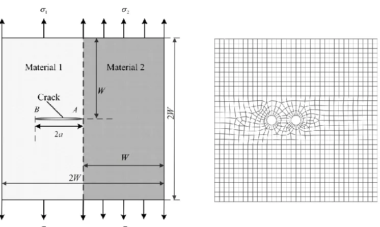
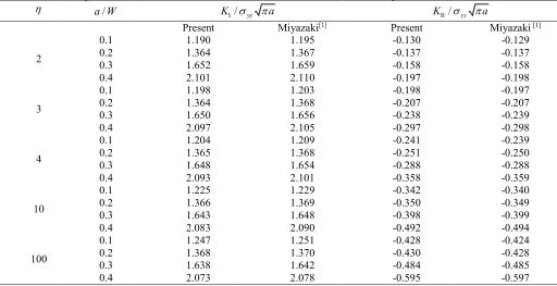
Example 1: Considering an edge cracked bimaterial plate under tensile loading as shown in Fig.5, in which the FE mesh of the plate is also provided. The ratio of the Young’s moduli of the two materials

is denoted by E E2/ 1. According to the previous study[40], a total of 25 export nodes of the SASE are

SIFs for different crack lengths are listed in Tab.1, and the numerical results of Ref.[1] obtained by

using BEM are listed for comparison. It is found that the present results agree well with these of Ref.[1],

and hence the present method is validated. Considering that the numerical results might be affected by

the size of the SASE, we take the special case where  2 and a W/ 0.1 as an example to study the

impact of the SASE’s size  on the solving accuracy. The present predictions as well as the reference

results[1] _on

I

K and KII are shown in Fig.6, it is shown that the present predictions are stable and

accuracy under a large range of the element size, and the reason for this satisfactory performance has

been explained in the section 7.2. The contours of the stresses around the crack tip are shown in Fig.7, in

which the stress concentration can be easily observed.

Example 2: Consider a square plate composed of two materials as shown in Fig.8, the geometric parameters are W 20 and a 1. The plate is subject to the tensile loading with 1E1 and 2 E2.

There are two crack tips in this model, and both of them are meshed using the present SASE. It may

noted that the crack at the point B is a single material crack, and the formulation of the SASE for this

problem has been reported in Ref.[46]. The present numerical predictions and the reference results of the

non-dimensional SIFs _{2 /(} 1 s₎

I y

K  a _{for the crack tip}

A and B are, respectively, listed in Tab.2 and

Tab.3. For the crack tip A, the eigenvalue which brings the stress singularity is denoted by s and also

listed in Tab.2. Again, good agreements are found between the present predictions and the reference

results from Refs[10, 11, 13].

1 0.3

  . The magnitude of the tensile loading is _y 1MPa. By using the SASE around the crack tip,

the SIFs are predicted for different crack orientations and the results are listed in Tab.4. The numerical

results obtained by using extrapolation method on the FE results with extremely refined mesh reported

in Ref.[17] are listed as a reference. According to the comparison, the present results agree very well

with the reference results. Moreover, the computing cost of the present method is much more cheaper. In

Ref.[17], the eight node plane element (quadratic element) is employed and a total of 382640 nodes are

used in the mesh. But in the present study, the four node plane element (linear element) and a SASE are

used and only 1425 nodes are used in the mesh.

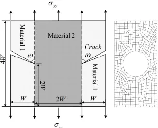
Example 4: Considering the double edge cracked 80mm 80mm bimaterial plate as shown in Fig.10, the magnitude of the tensile loading is _yy 1MPa. The ratio of the Young’s moduli of the two

materials is denoted by  E E2/ 1. The present predictions of the SIFs for different crack orientations

are listed in Tab.5, Tab.6 and Tab.7. The numerical results of single material case obtained by using the

quarter point singular element in the ANSYS software are also provided for comparison.

Example 5: Considering the structure as shown in Fig.11, the geometric parameters are given by 20mm

W  and a6mm, and the magnitude of the tensile loading is _yy 1MPa. The Poisson's ratios

of the two materials are  1= =0.22 . The ratio of the Young’s moduli of the two materials is denoted by

2/ 1

E E

 . Numerical results of the SIFs for crack the tip A and B are, respectively, listed in Tab.8

and Tab.9. Different crack orientations with _30o_{, 45 and} o _{90 are considered, and the values of} o

crack orientation angle  are specified in the brackets in the tables. It is interesting to find that with the

decrease. This prediction implies that the inclined interface crack is attracted to propagate towards the

stiffer material which is bounded to relatively softer material. And this trend is also affected by the

inclined angle of the crack, e.g., the variation of the SIFs is significant when _90o _{but remains}

relatively small when _30o_{. The numerical prediction could be used for the structure optimization of}

composite material for the case where the crack tends to propagate into the stiffer material, for example,

to release certain healing agent embedded in the composite material. It should be noted that this is not

within the scope of the present study and hence has not been addressed in this paper.

9.Conclusion

In this study, the inclined interface crack problem in composite has been investigated systematically

from theoretical and computational aspects. By using the symplectic approach, the explicit forms of the

eigen solution for the inclined interface crack were derived for the first time. The stress intensity factors

(SIFs) for the cracks along, perpendicular to, and inclined to the interface were determined. Moreover, a

new Symplectic Analytical Singular Element (SASE) has been developed based on the obtained

symplectic eigen solution. It has been found that the composites with complex geometric configurations

could be analyzed numerically by using the proposed SASE. In the worked examples, the first fifty

symplectic eigen expanding terms were selected in the SASE to capture the stress state around the crack

tip. Furthermore, the comparison between the present results and the benchmarks has indicated that the

developed model is very accurate in capturing the stress state around the inclined interface crack.

10.Acknowledgements

The supports of the National Natural Science Foundation of China (No.11502045, and No.

11372065), the Fundamental Research Funds for the Central Universities (DUT15RC(3)029) are

11.Appendix

The expression of matrix C (in this case the subscript i is omitted for simplicity) in the general

solution of the eigenvector is specified by

3

cos[(1 ) ] sin[(1 ) ] cos[(1 ) ] sin[(1 ) ] 3

3

sin[(1 ) ] cos[(1 ) ] sin[(1 ) ] cos[(1 ) ] 3

(3 ) (3 )

cos[(1 ) ] sin[(1 ) ] cos[(1 ) ] sin

1 1 3 3

E E E E

                                                                                   = C

[(1 ) ]

(1 ) (1 )

sin[(1 ) ] cos[(1 ) ] sin[(1 ) ] cos[(1 ) ]

1 1 3 3

E E E E

                                                                (A1)

It is proven that the matrix C still remains unchanged when 1.

In order to simplify the expressions, we define the parameters E E2/ 1 and  (13) /(11)

and introduce the Dundurs parameters[1]

1 2 2 1

1 2 2 1

( 1) ( 1)

( 1) ( 1)

G G G G         

   , 1_{1 2}2 2₂ 1₁

( 1) ( 1)

( 1) ( 1)

G G G G         

   (A2)

The coefficients A1, B1, C1 and D1 in the eigenvector of region #1 can be expressed by those of region

#2 with the following coefficients:









1 2







1



2









21



2









21



2





1 1 1 1 1 1 1 1

, , ,

2 1 2 1 2 3 2 3

p_   p_   p_   p_  

       

       

   

        (A3)

























 







 



























 







 



sin 2 1

1 cos 2 1

1 cos 2 1

sin 2 1

sin 2 cos 2

sin 2 cos 2



 









 









 



































 









 























 



















2 2 2 2

cos 2 2 sin 2

sin 2 cos 2 2

sin 2 1

1 cos 2 1

sin 2 1 1 cos 2 1

a a b b c c d d                                                                                                          _ _  _ _        _{ }  _{ }         (A5)

The coefficients A3, B3, C3 and D3 of the eigenvector of region #3 can be expressed by those of region

#2 with the following coefficients:































 





 









 





 







2 2 2 1 1 1 ₂ 1 a a c c b _b d _d      _  _                         _{     }     _{     }               _{  }  _{ }                 _{  }    _{ }       _{ }  _{   }            _{  } (A6)

Substituting the eigenvectors into the boundary conditions Eq.(22) and (23) gives









































2 2 2 2

2 2 2 2

2 2 2 2

2 2 2 2

cos 1

sin 1 1

cos 1

1

sin 1 0

a p A a p B a p C a p D

b p A b p B b p C b p D

c p A c p B c p C c p D

d p A d p B d p C d p D                                        _{  }    _{  }    _   _     _   _      _   _       _   _      (A7)









































2 2 2 2

2 2 2 2

2 2 2 2

2 2 2 2

sin 1

cos 1 1

sin 1

1

cos 1 0

a p A a p B a p C a p D

b p A b p B b p C b p D

c p A c p B c p C c p D

d p A d p B d p C d p D                                        _{  }    _{  }             _   _      _   _       _   _      (A8)









































2 2 2 2

2 2 2 2

cos 1 sin 1

1 1

cos 1 sin 1 0

a p A a p C b p B b p D

c p A c p C d p B d p D