City, University of London Institutional Repository
Citation
:
Cowell, R., Graversen, T., Lauritzen, S. L. and Mortera, J. (2014). Analysis of
forensic DNA mixtures with artefacts. Journal of the Royal Statistical Society. Series C:
Applied Statistics, doi: 10.1111/rssc.12071
This is the accepted version of the paper.
This version of the publication may differ from the final published
version.
Permanent repository link: http://openaccess.city.ac.uk/5764/
Link to published version
:
http://dx.doi.org/10.1111/rssc.12071
Copyright and reuse:
City Research Online aims to make research
outputs of City, University of London available to a wider audience.
Copyright and Moral Rights remain with the author(s) and/or copyright
holders. URLs from City Research Online may be freely distributed and
linked to.
Analysis of Forensic DNA Mixtures with Artefacts
R. G. Cowell
City University London, United Kingdom
T. Graversen
University of Oxford, United Kingdom
S. L. Lauritzen
University of Oxford, United Kingdom
J. Mortera
Universit `a Roma Tre, Italy
Summary. DNA is now routinely used in criminal investigations and court cases, although DNA samples taken at crime scenes are of varying quality and therefore present challenging problems for their interpretation. We present a statistical model for the quantitative peak infor-mation obtained from an electropherogram (EPG) of a forensic DNA sample and illustrate its potential use for the analysis of criminal cases. In contrast to most previously used methods, we directly model the peak height information and incorporate important artefacts associated with the production of the EPG. Our model has a number of unknown parameters, and we show that these can be estimated by the method of maximum likelihood in the presence of multiple unknown individuals contributing to the sample, and their approximate standard errors calculated; the computations exploit a Bayesian network representation of the model. A case example from a UK trial, as reported in the literature, is used to illustrate the efficacy and use of the model, both in finding likelihood ratios to quantify the strength of evidence, and in the de-convolution of mixtures for the purpose of finding likely profiles of the individuals contributing to the sample. Our model is readily extended to simultaneous analysis of more than one mixture as illustrated in a case example. We show that combination of evidence from several samples may give an evidential strength close to that of a single source trace and thus modelling of peak height information provides for a potentially very efficient mixture analysis.
Keywords: allelic dropout; Bayesian networks; DNA profiles; forensic statistics; gamma distri-bution; mixture deconvolution; strength of evidence; stutter.
1. Introduction
Since the pioneering work of Jeffreys et al. (1985), genetic fingerprinting or DNA profiling has become an indispensable tool for identification of individuals in the investigative and judicial process associated with criminal cases, in paternity and immigration cases, and other contexts (Aitken and Taroni, 2004; Balding, 2005). The technology has now reached a stage where uncertainty associated with determining the identity of an individual based on matching a high quality DNA sample from a crime scene to one taken under laboratory conditions has been virtually eliminated. Frequently, however, DNA samples found on
Address for correspondence: Steffen L. Lauritzen, Department of Statistics, University of Ox-ford, 1 South Parks Road, Oxford OX1 3TG, United Kingdom.
crime scenes are more complex, either because the amounts of DNA are tiny, even just a few molecules, the samples contain DNA from several individuals, the DNA molecules have degraded, or a combination of these. In such cases there is considerable uncertainty involved in determining whether or not the DNA of a given individual, for example a suspect in a criminal case, is actually present in the given sample. A sample found on the crime scene may contain material from the victim but also from individuals which might be involved in the crime, and determining their DNA becomes an important issue for the criminal investigation. In many cases suchmixed samples contain DNA from, say, a victim and a perpetrator, but advanced DNA technology now extracts genetic material from a huge variety of surfaces and objects which may have been handled by several individuals, only some of them being related to the specific crime. DNA mixtures with DNA from many individuals occur frequently in multiple rape cases or in traces left by groups of perpetrators handling the same objects such as, for example, balaclavas and crowbars.
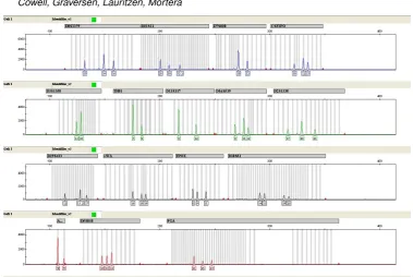
The basic representation of the composition of a DNA sample is the electropherogram (EPG), as described further in Section 1.1 below and displayed in Fig. 1. The identifi-cation of the DNA composition from the EPG information gives rise to a wide range of challenging statistical questions, some associated with uncertainties and artefacts in the measurement processes, some associated with population genetic variations, and other of a more conceptual nature. This article attempts to address some of these challenges.
As detailed in Section 3 below, the statistical issues concerning DNA mixtures have previously been addressed in a number of different ways. Some approaches make use only of the presence or absence of peaks in the EPG or use the peak heights in a semi-quantitative fashion; other approaches seek to develop fully quantitative models of observed peak heights. Although several methods have been developed, they each suffer from limitations of various kinds and none of the methods have been universally acknowledged as gold standards.
This article presents a new statistical model for the peak heights of an EPG. It builds upon earlier models presented in Cowell et al. (2007a,b, 2011) but is simpler than these, for example eliminating the need for previously introduced discretizations of some con-tinuous parameters. The simplifications of the model combined with an efficient Bayesian network representation (Graversen and Lauritzen, 2013a) enables fast computation and per-mits analysis of mixtures in which the presence of several unknown contributors is posited; in particular, estimation of unknown parameters by maximum likelihood becomes compu-tationally feasible.
corresponds to a proper allele or is due to anartefact of the measurement process such as, for example, stutter; see further in Section 1.1.2. It is also shown how the networks may be extended for other purposes. In Section 4.4 we show how the model can also be useful for the analysis of DNA from a single individual. Finally we discuss suggestions for further work in Section 5.
1.1. DNA mixtures
In this section we describe the nature of the information that we analyse with our DNA mixture model and give a brief description of the DNA amplification process and associ-ated measurements as carried out in forensic laboratories. We also introduce some of the complications that can occur. A more comprehensive description may be found in Butler (2005).
1.1.1. Short Tandem Repeat (STR) markers
Forensic scientists encode an individual’s genetic profile using the composition of DNA at various positions on the chromosomes.
A specific position on a chromosome is called a locus, ormarker. The information at each locus consists of an unordered pair ofalleles which forms thegenotype at that locus; a pair because chromosomes come in pairs, one inherited from the father and one from the mother, and unordered because it is not recorded from which chromosome of the pair each allele originates. We adopt the standard assumption that the population is in Hardy– Weinberg equilibrium implying that the two alleles of an individual can be assumed to be sampled independently from the same population. Human DNA has twenty three pairs of chromosomes: twenty two autosomal chromosome pairs and a sex-linked pair.
The loci used for forensic identification have been chosen for various reasons. Among these, we point out the following two. The first reason is that at each locus there is a wide variability between individuals in the alleles that may be observed. This variability can therefore be exploited to differentiate people. The second reason is that each locus is either on a distinct chromosome, or if a pair of loci are on the same chromosome then they are widely separated. This means that the alleles at the various loci may be treated as mutually independent, thus simplifying the statistical analysis.
The alleles of a marker are sequences of the four amino acid nucleotidesadenine, cyto-sine, guanine andthymine, which we represent by the letters A, C, G and T. Each amino acid is also called abase, and because the DNA molecule has a double helix structure, each amino acid on one strand is linked to a complementary amino acid on the other strand; a complementary pair of amino acids is called abase pair.
counts how many complete words of four bases make up the allele sequence but the words need not be all identical and may vary even within loci. For example, allele 11 of the marker VWA has the base sequenceT CT A[T CT G]3[T CT A]7. Also, some markers are based on tri-or pentanucleotide motifs rather than tetranucleotides as above. The base-letter sequences for many alleles may be found in Butler (2005).
When the repeat numbers of the two alleles of an individual at a marker are the same, then the genotype for that marker is said to be homozygous; when the repeat numbers differ, the genotype for that marker is said to beheterozygous.
The repetitive structure in the alleles gives rise to the term short tandem repeat (STR) marker to describe these loci; they also go by the name of microsatellites. Note that for other purposes of genetic analysis it is common to use single-nucleotide polymorphisms (SNPs) which are defined as DNA sequence variations that occur when a single nucleotide (A, T, C, or G) in the genome sequence is altered. However, for a number of reasons, the use of STR alleles is dominating in forensic genetics.
Within a population the various alleles of STR markers do not occur equally often, some can be quite common and some quite rare. When carrying out probability calculations based on DNA, forensic scientists use estimates of probabilities based on allele frequencies in profiles of a sample of individuals. The sample sizes typically range from a few hundred to thousands of individuals. For example, Butler et al. (2003) presents tables of US-population STR-allele frequencies for Caucasians, African-Americans, and Hispanics based on sample sizes of 302, 258 and 140 individuals.
1.1.2. The PCR process
Note that after breaking down the cell walls to release the chromosomes there could be sufficient DNA in the sample to carry out PCR amplifications with several extracts. When this is done it is called areplicate run.
To understand the quantification stage of the post PCR amplified DNA, it is important to know that the amplification process does not copy only the repeated DNA word segment of a marker, it also copies DNA at either end. These are calledflanking regions, and their presence is important in performing the PCR process. Thus an amplified allele will consist of the allele word sequence itself and two flanking regions, and will have a length associated with it which is measured in the total number of base pairs included in the word sequence and the flanking regions. For each marker, the DNA sequence (hence the size) forming each of the two flanking regions is constant, but different across markers. Thus quantifying a certain allele is equivalent to measuring how much DNA is present of a certain size. This is carried out by the process ofelectrophoresis, as follows.
The flanking regions have attached to them a fluorescent dye. Several colours of flu-orescent dyes are used to distinguish similarly sized alleles from different markers. The amplified DNA is drawn up electrostatically through a fine capillary to pass through a light detector, which illuminates the DNA with a laser and measures the amount of fluorescence generated. The latter is then an indication of the number of alleles tagged with the fluores-cent marker. The longer alleles are drawn up more slowly than the shorter alleles, however alleles of the same length are drawn up together. This means that the intensity of the detected fluorescence will sharply peak as a group of alleles of the same length passes the light detector, and the value of the intensity will be a measure of the number of alleles that pass. The detecting apparatus thus measures a time series of fluorescent intensity, but it converts the time variable into an equivalent base pair length variable. The data may be presented to a forensic scientist as anelectropherogram(EPG) as shown in Fig. 1 with each panel in the EPG corresponding to a different dye. The horizontal axes indicate the base pair length, and the vertical axis the intensity.
In the absence of artefacts, a peak in the EPG indicates presence of an allele in the sample before amplification. The peak height is a measure of the amount of the allele in the amplified sample expressed inrelative fluorescence units (RFU). The area of the peak is another measure of the amount, but this is highly correlated with the height (Tvedebrink et al., 2010). Both peak height and peak area are determined by software in the detecting apparatus.
We shall call the peak size information extracted from the EPG the profile of the DNA sample, or more briefly, the DNA profile. Commonly, DNA profile also refers to the com-bined genotype of a person across all markers.
Fig. 1.An electropherogram (EPG) using the IdentifilerTMSTR kit. Each of the four panels represents
a dye. Marker names are in grey boxes above panels and repeat numbers of detected alleles are given below the corresponding peaks. The vertical grey bars are used to identify alleles by their length in base pairs. On the left-hand side of each panel the scale of RFU is indicated.
Another artefact is known as dropin, referring to the occurrence of small unexpected peaks in the EPG. This can for example be due to sporadic contamination of a sample either at source or in the forensic laboratory.
Current technology allows for the amplification of very little DNA material, even as little as contained within one cell (Findlay et al., 1997). Amplifications of low amounts of DNA are termed low template DNA (LTDNA). LTDNA analyses are particularly prone to artefacts such as dropin and dropout.
Finally, a mutation in the flanking region can result in the allele not being picked up at all by the PCR process, in which case we say that the allele issilent. An allele can also be undetectable and thusde facto silent because its length is off-scale and the peak does therefore not appear in the EPG.
1.2. Motivating example
As a motivating example we shall consider a case from a UK trial as reported in Gill et al. (2008), also analysed in Cowell et al. (2011):
Table 1.Alleles, peak heights, and genotypes of individu-als for an excerpt of the markers in the pub crime case.
Marker Alleles MC18 MC15 K1 K2 K3
D2 16 189 64 16
17 171 96 17
22 55 0
23 638 507 23
24 673 524 24 24
D16 11 534 256 11 11
12 1786 1724 12 12
13 265 109 13
TH01 7 670 727 7
8 636 625 8
9 99 0 9
9.3 348 165 9.3
alleged offenders then left the scene and went to another public house where they were seen to go into the lavatory to clean themselves.”
Two blood stains, MC18 and MC15, were found at the public house lavatory. Both indicated that they were DNA mixtures of at least three individuals. The genotypes of the defendant,K3, and a known individual,K2, alleged to be present at the time of the offence, were determined together with that of thevictim K1 (all were males). An excerpt of the observed DNA profiles of the samples and individual genotypes are displayed in Table 1. The complete data can be found in Gill et al. (2008) and in the R-packageDNAmixtures
(Graversen, 2013).
Note that if the trace consists of DNA from exactly K1,K2, andK3, the peak at allele 22 of marker D2 in MC18 would need to be due to stutter and/or spontaneous dropin, and
K2’s allele 9 on marker TH01 would have dropped out of the MC15 profile. We emphasize that the entire profile would be consistent with only DNA from K1, K2, and K3 being present in the traces.
1.3. Objectives of analysis
The analysis of a DNA profile can have different objectives depending on the context. The objective can be a quantification of the strength of evidence for a given hypothesis over another, or the objective may be adeconvolution of the profile,i.e. one wishes to identify likely genotypes of contributors (Perlin and Szabady, 2001; Wang et al., 2006; Tvedebrink et al., 2012a). We briefly describe the typical situations below.
Weight of evidence The availableevidence E consists of the peak heights as observed in the EPG as well as the combined genotypes of the known individuals. It is customary to assume relevant population allele frequencies to be known. We shall return to this issue in Section 5.
To quantify the strength of the evidence against the defendant (K3), two competing hypotheses are typically specified. One of these, usually referred to as the prosecution hypothesis Hp, could in our example be that the profile has exactly three contributors who
as known contributors in addition to one or more unknown individuals who we shall name
U1, U2, U3, . . .and refer to asunknown contributors. The alleles of the unknown contributors are assumed to be chosen randomly and independently from a reference population with known allele frequencies. To limit the scope of our analysis we shall here only consider scenarios which includeK1 andK2as contributors to the traces.
The prosecution hypothesis is then compared to what is referred to as the defence hypothesis Hd, which typically would replace K3 in Hp with an unknown contributor,
claiming that the apparent similarity between the trace and the DNA profile ofK3is due to chance. The defence hypothesis is not actually advocated by the defence, but is formulated strictly for comparative purposes. We emphasize that this implies that the genotypes of this unknown contributor in principle could be identical to that ofK3 although this would be extremely improbable, ignoring cases involving identical twins.
The strength of the evidence (Good, 1950; Lindley, 1977; Balding, 2005) is normally represented by thelikelihood ratio:
LR= L(Hp)
L(Hd)
= Pr(E| Hp) Pr(E| Hd) .
We shall follow Balding (2013) and report the weight of evidence as WoE = log10LR in the unitban introduced by Alan Turing (Good, 1979) so that one ban represents a factor 10 on the likelihood ratio. For a high quality single source DNA profile (i.e. from a single individual) in the SGM Plus system, values for WoE vary around 14 bans (Balding, 1999), which in most cases would be considered sufficient for establishing the identity of the individual leaving the stain. We emphasize that this unit of WoE is not absolute, but should be always be interpreted relative to a specific defence hypothesis; it could for example change — in principle in any direction — if alsoK2were replaced by an unknown individual.
The calculation of the WoE can be important both when presenting a case to the court and in the investigative phase of a trial, to decide whether it is worthwhile to search for additional independent evidence.
The numerator and denominator in the likelihood ratio are calculated based on models which shall be detailed further in Section 2 below; generally models have the form
Pr(E| H) =X
g
Pr(E|g) Pr(g| H)
so that the model for the conditional distribution Pr(E|g) of the evidence given the geno-typesgof all contributors is the same for both hypotheses, whereas the hypotheses differ concerning the distribution Pr(g| H) of genotypes of the contributors, as described above.
Deconvolution of DNA mixtures This calculation attempts to identify the combined geno-types across all markers of each unknown contributor to the mixture and give a list of potential genotypes of a perpetrator to use for a database search. For example, we could wish to calculate
Pr{U1, U2|E,Hinv} or Pr{U1|E,Hinv},
Evidential efficiency For a single source high quality trace the WoE specializes to −log10 of thematch probability i.e. the probability that a random member of the population has the specific DNA profile ofKs (Balding, 2005). We point out that the WoE against a suspect
Ks based on our model can never be stronger than the WoE obtained by a single source DNA profile. To see this, let πs = Pr(U = Ks) denote the match probability. Further, let Hp be the prosecution hypothesis involving Ks as a contributor and Hd the defence
hypothesis, replacing the genotypeKsby that of a random individualU. We then have
LR=Pr(E| Hp) Pr(E| Hd)
= Pr(E| Hp)
Pr(E| Hd, U =Ks)πs+ (1−πs) Pr(E| Hd, U6=Ks)
= Pr(E| Hp)
Pr(E| Hp)πs+ (1−πs) Pr(E| Hd, U 6=Ks)
≤ Pr(E| Hp) Pr(E| Hp)πs
= 1
πs
. (1)
Thus we have WoE = log10LR ≤ −log10πs implying that a mixed trace can never give stronger evidence than a high-quality trace from a single source. We define the loss of evidential efficiency WL(E|Ks) against Ks in the evidenceE as
WL(E|Ks) = WoE(Ks)max−WoE(Ks) =−log10πs−log10
Pr(E| Hp)
Pr(E| Hd) .
This quantity is non-negative, and indicates how many bans of WoE are lost due to the evidence being based on a mixture rather than a single source trace. Indeed, the loss of efficiency for a mixed trace can be compared to the loss induced by failure of identifying the genotype for some markers, as this increases the match probability in a similar way. For the case example in Section 1.2, using the US Caucasian allele frequencies of Butler et al. (2003), the negative logarithm of the match probability forK3is−log10πK3 = 14.5,
whereas if we ignored, say, markers D18 and D19, the weight-of-evidence would be WoE = −log10π˜K3 = 12.0, losing about 2.5 bans.
In the case of deconvolution without a specified suspect, we could consider the evidence against the posterior most likely unknown personK∗ under the defence hypothesis. IfH∗
p
denotes a prosecution hypothesis obtained by replacingUwithK∗andπ∗= Pr(U =K∗) = Pr(U =K∗| Hd) denotes the prior probability of a random individual having genotypeK∗,
we get
WL(E|K∗) = −log10π∗−log10Pr(E| H ∗
p)
Pr(E| Hd)
=−log10Pr(E| H ∗
p)π∗
Pr(E| Hd)
= −log10Pr(E|U =K ∗,H
d) Pr(U =K∗| Hd)
Pr(E| Hd)
= −log10Pr(U =K∗| Hd, E). (2)
Thus, thisgeneric loss of evidential efficiency is equal to−log10of the maximum posterior probability obtained in the deconvolution. For a single source trace that uniquely identifies the contributor, the generic loss of evidential efficiency is 0.
2. A gamma model with artefacts
In this section we present an overview of the basic model for peak heights, which is based on the gamma model described in Cowell et al. (2007a) and used in Cowell et al. (2011) with extensions describing artefacts. It should be emphasized that the model used here is different from the latter in two main respects: firstly it uses absolute peak heights instead of relative peak heights which enables direct treatment of dropout by thresholding; secondly, it has a different description of stutter. As a consequence, computations are greatly simplified so analysis is possible for a high number of unknown potential contributors.
2.1. Basic model
We consider I potential contributors to a DNA mixture. Let there beM markers used in the analysis of the mixture with marker m having Am allelic types, m = 1, . . . , M. Let
φi denote the fraction of DNA from individual i prior to PCR amplification, with φ = (φ1, φ2, . . . , φI) denoting the fractions from all contributors. Thusφi≥0 andP
I
i=1φi= 1. For identifiability of the parameters we further assume that the fractions φi for unknown contributors are listed in non-increasing order, i.e. φa ≥ φb if a < b are both unknown individuals. It is assumed that these pre-amplification fractions of DNA are constant across markers.
For a specific marker mand allelea, the model is describing the totalpeak height Ha. Ignoring artefacts for the moment, the model makes the following further assumptions: Each contribution Hia from an individual i to the peak height at allele a has a gamma
distribution,Hia∼Γ(ρφinia, η), where Γ(α, β) denotes the distribution with density
f(h|α, β) = h
α−1 Γ(α)βαe
−h/β forh >0.
Forα= 0, Γ(0, β) is the distribution degenerate at 0. Hereρis proportional to the total amount of DNA in the mixture prior to amplification; the number of alleles of typeacarried by individualiis denoted bynia; and the parameterη determines the scale. We note that
the individual contributionsHiaare unobservable. Indeed, when artefacts are added to the
model, the peak heightsHa=P
iHiathemselves are unobserved; they will be modified by
stutter and dropout as described below in Section 2.2.
For notational simplicity we have suppressed the dependence of the heights Hm ia and
other quantities on markers m. It is important for the model that φi are the same for all markers, whereas one would typically expect other parameters to be marker dependent and possibly dependent on fragment length in case of degraded DNA (Tvedebrink et al., 2012b). We note that the assumption of a common scale parameterηm for the individual contributionsHiamfor different allelesaenables a simple interpretation of the model in terms of adding independent contributions to peaks both from proper alleles and from stutter, see below.
It becomes practical to introduce theeffective numberBa(φ,n)of alleles of typeawhere Ba(φ,n) =Piφinia, andn= (nia, i= 1, . . . I;a = 1, . . . , A); we note that as Piφi = 1,
we have that P
aBa(φ,n) is constant over markers and equal to two in the diploid case.
As a sum of independent gamma distributed contributions, the peak heightHa at allele ais gamma distributed as
Ha ∼Γ{ρBa(φ,n), η}. (3)
The distribution of Ha has expectation ρηBa(φ,n) and variance ρη2Ba(φ,n). Thus the mean ofHais approximately proportional to the amount of DNA of typeaand the variance is proportional to the mean. We letµ=ρη and σ= 1/√ρ. Then — in a trace with only one heterozygous diploid contributor and no artefacts —µis the mean peak height and σ
the coefficient of variation for peak heights; hence σ becomes a measure of generic peak imbalance. In the presentation of results we shall often use (σ, µ) instead of (ρ, η) because of their more direct interpretability.
2.2. Incorporating artefacts
The model described above does not incorporate a number of important artefacts as de-scribed in Section 1.1. This section is devoted to the necessary modifications needed to take these into account.
Stutter We represent stutter by decomposing the individual contributions Hia to peak heights in the EPG intoHias andHia0 so that
Hia=Hias +Hia0
whereHias represents the DNA originating from individualiof allelic type athat stutters toa−1 by losing a repeat number, andHia0 represents the remainder that goes through the PCR process undamaged. We let the components be independent and gamma distributed as
Hias ∼Γ{ρξφinia, η}, Hia0 ∼Γ{ρ(1−ξ)φinia, η},
whereξis themean stutter proportion. The total peak height observed at allele ais then
Ha =
X
i
Hia0 +X
i
Hi,as +1=Ha0+Has+1.
Note that nowHa has a slightly different meaning than in (3) above as it has potentially
received stutter from the allele above and lost stutter to the allele below. We ignore the possibility that Ha might have tiny stutter contributions Has+2, Has+3,· · · from peaks at
a+ 2, a+ 3, . . .. Including this is straightforward in principle, but it has strong effects on the complexity of computations (Graversen and Lauritzen, 2013a). The new peak height
Ha is also gamma distributed as
Ha∼Γ{ρDa(φ, ξ,n), η}
where now
Da(φ, ξ,n) = (1−ξ)Ba(φ,n) +ξBa+1(φ,n) (4)
are theeffective allele counts after stutter. Here and elsewhere we have letBA+1(φ,n) = 0. The relative contribution lost to stutter
Xa = H
s a Hs
thus follows a beta distributionB{ξρBa(φ,n),(1−ξ)ρBa(φ,n)}with mean E(Xa) =ξ.
Notice that our use of stutter proportion Xa differs from standard practice which uses
the ratio between the stutter peak and the parent peak (Butler, 2005). A peak in stutter position may itself include contributions from proper alleles, and the parent peak may itself include stutter contributions from an allele with higher repeat number. Even in the simple event that a peak is entirely due to stutter from a parent peak, which has not itself been inflated by stutter, we haveHa=H0
a andHas=Ha−1and thus ourXa =Ha−1/(Ha−1+Ha) rather than the conventionalHa−1/Ha.
Dropout The next step in our model is concerned with the fact that in mixtures some alleles are not observed; either because no peak can be identified, or because the peak is below some detection threshold. This phenomenon is prominent for small amounts of DNA. Here we take the consequence of the model and represent dropout by a total peak height below the chosen thresholdC, as described in Section 1.1. In other words, we do not observe the heightHa as just described, but ratherZa, where
Za=
Ha ifHa≥C
0 otherwise.
This implies that the probability that a specific allele is not observed is
P(Za = 0|n) =G{C;ρDa(φ, ξ,n), η},
whereGdenotes the cumulative distribution function of the gamma distribution.
Allelic dropout for single source traces was studied by Tvedebrink et al. (2009, 2012) who fitted a logistic regression model to the dropout probability as
P(Za= 0|h¯) = α ¯
hβ
1 +α¯hβ (5)
where ¯his an average of observed peak heights above threshold calculated across all markers. They found that one could use the same value ofβ=−4.35 for all markers, whereasαwas marker dependent. The independent variable ¯hwas used as a proxy for total amount of DNA.
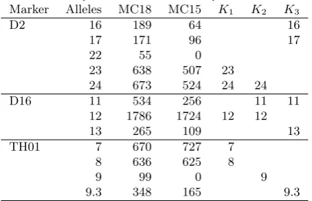
In our model, the theoretical mean peak height µ = ρη would be a similar proxy for the total amount of DNA. To compare the two models, we assume that ¯happroximately corresponds to the mean peak heightµ. Thus our model has
P(Za = 0|µ) =G{C;µ/η, η}, (6)
which can then be compared with (5) where ¯his replaced byµ. A selection of curves (6) for
C= 50 and values ofη corresponding to the maximum likelihood estimate and upper and lower 99% confidence limits in our case example, see Section 4; together with curves (5) for
β =−4.35 and representative values of α, are superimposed in Fig. 2. We note that the dropout model based on the gamma distribution tends to have lower dropout rates than the logistic model for small amounts of DNA.
0 50 100 150 200 250
0.0
0.2
0.4
0.6
0.8
1.0
Mean peak height
Dropout probability
η =16 η =28 η =40 α =17.4
α =18.4 α =19.4
[image:14.490.88.426.66.279.2]Gamma model Tvedebrink et al. 09
Fig. 2. The probability of dropout of a single allele as a function of mean peak height. The curves with full lines correspond to our gamma model whereas the dashed curves correspond to the logistic model.
threshold model — hence also for our gamma model — since if peak height contributions
Y1 andY2 from each allele are independent and identically distributed, we have
D=P(Y1+Y2< C)< P(Y1< C)2=d2.
For the model (5) we have
d
1−d =α
¯
hβ; D
1−D =α(2¯h)
β= 2β d
1−d
and thus
D= 2
βd
1 + (2β−1)d (7)
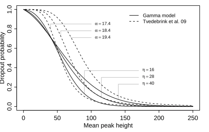
independently of the value of α. The curve in (7) is displayed in Fig. 3 for β = −4.35 together with the upper bound D =d2 and a selection of curves from the gamma model with C = 50 and the same values for η as in Fig. 2. We note that although (7) actually just crosses the curve D = d2 for very small values of d, this has hardly any practical significance, as also pointed out in Tvedebrink et al. (2012).
0.0 0.2 0.4 0.6 0.8 1.0
0.0
0.2
0.4
0.6
0.8
1.0
Heterozygous dropout probability (d)
Homozygous dropout probability (D)
η =16 η =28 η =40
[image:15.490.82.407.72.276.2]D=d2 Gamma model Tvedebrink et al. 09
Fig. 3.The probability of homozygous dropoutDas a function of the dropout probability of a single allele for the gamma model and for the logistic model of Tvedebrink et al. (2009). The solid curves
correspond to the gamma model for different values ofη.
modelled dropout entirely as a threshold phenomenon, ignoring the fact that apparatus failure could be an alternative explanation.
2.3. Joint likelihood function
For given genotypes of the contributors n, given proportions φ, and given values of the parameters (ρ, ξ, η), all observed peak heights are independent. Thus, the conditional like-lihood function based on the observationsz={zma, m= 1, . . . , M;a= 1, . . . , Am}for all markersm and allelesais
L(ρ, ξ, φ, η|z,n) =Y
m
Y
a
Lma(zma)
where
Lma(zma) =
g{zma;ρDa(φ, ξ,n), η} ifzma≥C G{C;ρDa(φ, ξ,n), η} otherwise,
withgandGdenoting the gamma density and cumulative distribution function respectively andDa are the effective allele counts after stutter in (4). For simplicity of notation, we have suppressed potential marker and allele dependence ofρ,η, andξin the above formulae.
For a given hypothesis H, the full likelihood is obtained by summing over all possible combinations of genotypesnwith probabilitiesP(n| H) associated with the hypothesis to give
L(H) = Pr(E| H) =X
n
The number of terms in this sum is huge for a hypothesis which involves several unknown contributors to the mixture, but can be calculated by Bayesian network techniques (Gra-versen and Lauritzen, 2013a); some details are given in Section 2.4 below.
Estimating unknown parameters The likelihood function L(H) involves a number of pa-rameters (ρ, ξ, φ, η) which may be completely or partially unknown.
One way of dealing with this is to make the likelihood as large as possible for each of the competing hypotheses and thus calculate
ˆ
L(H) = sup
ρ,ξ,φ,η
X
n
L(ρ, ξ, φ, η|z,n)P(n| H),
corresponding to using maximum likelihood estimates for the unknown parameters, but different estimates under the competing hypothesis. Since the likelihood function (8) can be efficiently computed, it is feasible to maximize it using appropriate numerical optimization methods.
Using maximized likelihood ratios preserves the property that the WoE against a suspect
Ksin a mixed trace based on our model can never be stronger than what is obtained by a matching single source DNA profile. To see this, recall thatπs= Pr(U =Ks) denotes the match probability,i.e. the probability that a random individual has the genotype of the suspectKs. As before, letHpbe the prosecution hypothesis, involvingKsas a contributor
and Hd be the defence hypothesis, replacing Ks by a random individual U. Let further
ˆ
ψp= ( ˆρp,ξp,ˆ φp,ˆ ηpˆ ) be the maximum likelihood estimates of the unknown parameters under the prosecution hypothesis and ˆψd the estimates under the defence hypothesis. We then have
WoE(Ks|ψd,ˆ ψdˆ ) = log10
Pr(E| Hp,ψˆd)
Pr(E| Hd,ψˆd)
≤log10
Pr(E| Hp,ψˆp)
Pr(E| Hd,ψˆd)
= WoE(Ks|ψˆp,ψˆd)≤log10
Pr(E| Hp,ψˆp)
Pr(E| Hd,ψpˆ ) = WoE(Ks|ψp,ˆ ψpˆ )≤ −log10πs= WoE(Ks)max,
where the last inequality is obtained as in (1). Thus, also when parameters are estimated, a mixed trace can never give stronger evidence than a high-quality trace from a single source.
2.4. Computation
Representation of genotypes As customary we assume a reference population in Hardy-Weinberg equilibrium so we can consider the two alleles of an individual chosen at random with allele frequencies (q1, . . . , qA). We recall from Section 2.2 that the distribution of peak height at alleleadepends on bothniaandni,a+1for both known and unknown contributors
i. To enable simple computation of the terms in the likelihood function (8), we therefore represent the genotype for contributori by a vector of allele counts (ni1, . . . , niA). These vectors then follow independent multinomial distributions withP
ania= 2.
Using properties of the multinomial distribution we can describe this distribution se-quentially as follows. The number ni1 of the first allelic type follows a binomial distri-bution Bin(2, q1). Denote by Sia = Pb≤anib the number of alleles of type 1 to a that
contributor i possesses. For any subsequent allelic type a+ 1, it holds that, condition-ally on Sia, the number of alleles of type a+ 1 is independent of the specific alloca-tions (ni1, . . . , nia) already made. Furthermore, ni,a+1 is also binomially distributed with
ni,a+1|Sia∼Bin(2−Sia, qa+1/Pb≥a+1qb). Thus, adding the partial sums of allele counts
to the network allows the genotype to be modelled by a Markov structure as displayed in Fig. 4.
Si1 Si2 Si3 Si4 Si5 Si6
ni1 ni2 ni3 ni4 ni5 ni6
O1 O2 O3 O4 O5 O6
nj1 nj2 nj3 nj4 nj5 nj6
Sj1 Sj2 Sj3 Sj4 Sj5 Sj6
Genotype for unknown contributori
Genotype for unknown contributorj
Partial sums of allele counts
Partial sums of allele counts
Fig. 4.Bayesian network modelling the genotypes of 2 unknown contributorsiandjand peak height observations for a marker with 6 possible allelic types.
Including peak height information The information about peak height observations is in-corporated via binary nodesOa in Fig. 4; these represent whether a peak for allelea has been seen. By suitable specification of the conditional distribution ofOa given its parent nodes, conditioning onOa being TRUE or FALSE will correspond to conditioning on the observed peak heightsZa; this enables in particular fast evaluation of the likelihood function (8) by a single propagation in the Bayesian network (Graversen and Lauritzen, 2013a).
The computational effort is exponential in the number of unknown contributors. How-ever, the Markov representation of the genotypes themselves ensures the complexity to grow linearly with the number of allelic typesA, rather than polynomially as in previously used representations (Cowell et al., 2007a,b, 2011).
current version of DNAmixtures, RHugin, and HUGIN. The computation time increases with the number of unknown contributors; the maximization of the likelihood function for five unknown contributors used around three hours on the same machine. Maximization of the likelihood function for six unknown contributors as used in Fig. 8 was done on a machine with more memory. See Graversen and Lauritzen (2013a) for further discussion of the computational issues.
3. Related literature
Methods for the interpretation of DNA profiles arising from mixtures can be classified into:
a) those mostly based on qualitative information,i.e. information about allele presence or absence in the DNA mixture;
b) those that also use quantitative information by taking into account both allele presence and peak intensities.
We will first discuss some recent relevant papers that base their model prevalently on allele presence and secondly we describe those that also exploit the information in the peak intensities. A list of publications relating to DNA mixtures is maintained at the website of the National Institute of Standards and Technology (NIST)†.
3.1. Methods based on qualitative information
Recently, the International Society for Forensic Genetics published recommendations based on discrete models for forensic analysis of single source DNA profiles (Gill et al., 2012). They consider a single locus (DNA marker) and at that locus allow for artefacts such as dropin and dropout, including the probability of their occurrence in the likelihood ratio computations. Under the independence assumptions of this model, they state that it readily extends to multiple loci and DNA mixtures. Gill et al. (2012) is largely based on Curran et al. (2005) and Balding and Buckleton (2009).
Curran et al. (2005) give a set based method for likelihood ratio calculations which in-cludes multiple contributors and the analysis of replicate runs. This was an improvement on previous guidelines for the analysis of LTDNA profiles where alleles were not reported unless they were duplicated in replicate runs (Gill et al., 2000). They consider the proba-bility of contamination and dropout, but not of stutter. The model is implemented in Gill et al. (2007). For the interpretation of LTDNA, Gill et al. (2008) include the probabilities of dropout, contamination and stutter; peaks in stutter positions are considered ambiguous alleles and included in the calculation. Furthermore, they account for dropin by increasing the number of potential contributors to the mixture. They also study the robustness of the WoE to misleading evidence in favour of the prosecution.
Balding and Buckleton (2009) consider a discrete model for interpreting LTDNA mix-tures where peaks are classified as present, absent, or masking. The set of masking alleles is defined as every peak above a designated threshold that either corresponds to an allele of a known contributor, is in a stutter position to that allele or to another peak of sufficient height. Based on an extension of this paper (Balding, 2013), Balding wrote a suite of R
functions likeLTD‡built for a range of crime scene DNA profiles, involving complex mix-tures, uncertain allele designations, dropin and dropout, degradation, stutter, relatedness of alternative possible contributors, as well as replicated runs. Alleles are defined as present, absent, or uncertain; dropout is modelled using Tvedebrink et al. (2009, 2012). Haned et al. (2011) estimate dropout probabilities using different logistic models for haploid and diploid cells in combination with a simulation model of the PCR process (Gill et al., 2005). Simi-larly, Haned et al. (2012) and Haned and Gill (2011) adopt a model based on allele presence that analyses the sensitivity to dropin and dropout parameters. The papers mentioned in this paragraph do not make direct use of peak heights, but peak heights enter implicitly in the process of allele classification.
3.2. Methods based on quantitative information
Early attempts to exploit peak intensity information include Evett et al. (1998); Perlin and Szabady (2001); Wang et al. (2006); Bill et al. (2005); and Curran (2008). Cowell et al. (2007a) introduced the use of gamma distributions to model peak area variability observed in the PCR amplification of DNA in mixtures, and presented a normal-approximation ver-sion of the model in Cowell et al. (2007b). Both of these papers carry out calculations using exact propagation algorithms for Bayesian networks, but require discretization of a parameter representing the relative amounts of DNA from each contributor to the mixture. Both evidential and deconvolution analyses were presented. The suitability of the gamma distribution was investigated in Cowell (2009), using the simulation model of Gill et al. (2005).
The gamma model of Cowell et al. (2007a) was extended in Cowell et al. (2011) to handle stutter, dropout and silent alleles. Stutter was represented in Bayesian networks by means of a discretization to allow probability propagation. The authors showed how the Bayesian network representation readily enabled the simultaneous analysis of two DNA mixtures that are thought to have contributors in common. The authors noted that the computational complexity of the model increased significantly with the total number of contributors, limiting the practical use of their methods to at most four contributors.
Perlin et al. (2011) present a model for DNA mixture interpretation based on a normal model extending the method in Perlin and Szabady (2001) in a direction similar to Cowell et al. (2007b). They use a fully Bayesian approach where all parameters are given a prior distribution. The model is used both for identification of contributors to a DNA mixture and for deconvolution. The model does not incorporate stutter, and dropout is accounted for by a background variance parameter. The performance of the model is reported for 16 two-person mixture samples, however the performance for mixtures of DNA from more than two people is not reported.
Puch-Solis et al. (2013) is based on using the gamma distribution for peak heights as in Cowell et al. (2007a, 2011). Since DNA degrades more the greater the DNA fragment length (Tvedebrink et al., 2012b), they use a correction for this phenomenon. Their methodology is different to the one presented here in that: i) they exploit the common scale parameter for peak heights to derive Dirichlet distributions for relative peak heights; ii) they use a pre-processing step for classifying peaks as possible stutter peaks; iii) they use a more complex dropout model; iv) they discretize the parameter representing the proportion of DNA from each contributor and use a finer grid on extreme intervals to better capture unbalanced
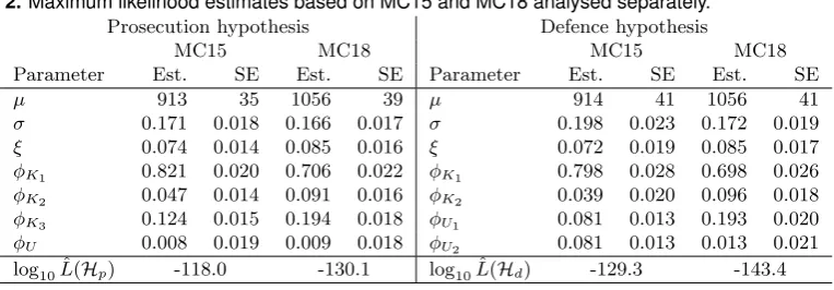
Table 2.Maximum likelihood estimates based on MC15 and MC18 analysed separately.
Prosecution hypothesis Defence hypothesis
MC15 MC18 MC15 MC18
Parameter Est. SE Est. SE Parameter Est. SE Est. SE
µ 913 35 1056 39 µ 914 41 1056 41
σ 0.171 0.018 0.166 0.017 σ 0.198 0.023 0.172 0.019
ξ 0.074 0.014 0.085 0.016 ξ 0.072 0.019 0.085 0.017
φK1 0.821 0.020 0.706 0.022 φK1 0.798 0.028 0.698 0.026
φK2 0.047 0.014 0.091 0.016 φK2 0.039 0.020 0.096 0.018
φK3 0.124 0.015 0.194 0.018 φU1 0.081 0.013 0.193 0.020
φU 0.008 0.019 0.009 0.018 φU2 0.081 0.013 0.013 0.021
log10Lˆ(Hp) -118.0 -130.1 log10Lˆ(Hd) -129.3 -143.4
mixtures; v) all alleles not corresponding to peaks above threshold are lumped together into a single compound allele. They discuss identification of contributors to the mixture and not deconvolution. The paper presents examples of two person mixtures and does not analyze replicate runs or multiple traces.
Tvedebrink et al. (2010) evaluate the weight of evidence for two person mixtures, using a multivariate normal distribution of peak heights. Based on DNA mixtures from controlled experiments they find a linear relationship between peak height and area and between means and variances of peak height measurements. Controlled experiments are also used for estimating the probability of allelic dropout per locus using logistic regression (Tvedebrink et al., 2009, 2012).
Recently, Taylor et al. (2013) used a log-normal model for the ratio between observed and expected peak heights.
4. Case analysis
We proceed to illustrate the methodology developed in Section 2 by applying it to the case described in Section 1.2. We have used a threshold of C = 50 for both traces MC15 and MC18; note that for MC18 the peaks for alleles 21 and 25 at marker FGA are of height 49 and 39 and thus below the threshold. Using a threshold ofC= 39 for this profile makes a negligible difference to the results.
The computations were all performed with the R-package DNAmixtures (Graversen, 2013) which is available from dnamixtures.r-forge.r-project.org. The R-package in-terfaces the HUGIN API (Hugin Expert A/S, 2012) through the R-packageRHugin(Konis, 2012). The likelihood functions are maximized numerically using Rsolnp (Ghalanos and Theussl, 2012; Ye, 1987). Approximate standard errors of estimates are based on the inverse Hessian of the likelihood function found by numerical derivation usingnumDeriv (Gilbert and Varadhan, 2012). The population allele frequencies used were taken from the US Cau-casian database in Butler et al. (2003).
4.1. Weight of evidence
parameters (µ, σ, ξ) are very similar under the two hypotheses, the defence hypothesis sug-gesting a slightly larger coefficient of variation, both a little less than 20%, i.e. indicating large variability of the peak heights. The mean stutter proportion ξ is estimated to just under 7.5%. The estimates of the contributor fractionsφunder the prosecution hypothesis agree well with the estimates (0.80,0.06,0.12,0.04) found in Table 3 of Gill et al. (2008). The resulting WoE is log10(LR) = −118.0−(−129.3) = 11.3 bans. For the prosecution hypothesis we can ignore spontaneous dropin, the standard deviation ofφU indicating this may well be zero. Under the defence hypothesis there are difficulties distinguishing the two unknown contributors in that their contributor fractions are estimated to the same value. Since the estimates for φUi are on the boundary of the parameter space, their standard errors are given for the model which further restricts them to be equal asφU1 =φU2.
Re-moving one unknown contributor for both hypotheses increases the WoE to 12.1 bans. This should be compared to the analysis in Cowell et al. (2011) which for hypotheses with three contributors gave a WoE around 10 bans. It should also be compared to the upper bound of 14.5 bans calculated from the match probability forK3.
Thus our model gives considerably stronger WoE than found previously, although much less than would have been possible for a perfect single source trace. The loss of efficiency compared to a single source trace is similar to the loss from leaving out, for example, markers D18 and D19; see Section 1.3.
Analysis of MC18 The maximum likelihood estimates and their approximate standard errors under the defence and prosecution hypotheses are given in Table 2.
We note again that the estimates for (µ, σ, ξ) are very similar under the two hypotheses, the defence hypothesis suggesting a slightly larger coefficient of variation, but the same order of magnitude as for MC15. Also here the estimates of the contributor fractions
φ under the prosecution hypothesis agree well with the estimates (0.67,0.11,0.19,0.04) in Table 2 of Gill et al. (2008). In contrast to MC15, the defence hypothesis identifies an unbalanced contribution to MC18 from the unknown contributors, the major unknown contributor representing a fraction similar to that of the defendantK3under the prosecution hypothesis. The estimates of the mean stutter proportions are slightly larger than found for MC15, although the standard errors suggest that the differences are well within what could be expected from random variation. The resulting WoE for this trace becomes 13.3 bans, which compares to losing the information in marker D18, say.
Standard deviations for contributor fractions indicate that one unknown contributor can be removed for both hypotheses; this has no essential effect on the WoE which remains at 13.3 bans. We compare again to Cowell et al. (2011) which gave a WoE around 10 bans, again a weaker evidential value than what we obtain from our model.
Combined analysis of MC15 and MC18 The combined analysis of more than one DNA profile can be very informative when computing the WoE but especially for deconvolution of mixed traces, see for example Section 4.2. This is particularly true when there might be high dropout probabilities in one or more of the profiles. Multiple profiles with the same contributors can, for example, be obtained from different parts of a crime stain, but also from different stains found at the same scene. In addition, as we shall see, the combined analysis may considerably improve the precision of parameter estimates.
Table 3.Maximum likelihood estimates when information in the traces MC15 and MC18 is combined.
Prosecution hypothesis Defence hypothesis
MC15 MC18 MC15 MC18
Par. Est. SE Est. SE Par. Est. SE Est. SE
µ 914 36 1055 38 µ 914 36 1055 39
σ 0.175 0.013 0.163 0.012 σ 0.178 0.013 0.165 0.013 ξ 0.079 0.011 0.079 0.011 ξ 0.079 0.011 0.079 0.011 φK1 0.822 0.020 0.705 0.021 φK1 0.820 0.021 0.702 0.023
φK2 0.048 0.014 0.090 0.016 φK2 0.049 0.014 0.091 0.017
φK3 0.125 0.016 0.193 0.018 φU1 0.123 0.016 0.193 0.018
φU 0.006 0.018 0.012 0.017 φU2 0.008 0.019 0.014 0.018
log10Lˆ(Hp) -248.2 log10Lˆ(Hd) -262.3
contributors to the two traces are different and unrelated. Under this assumption, the traces are independent and the joint likelihood ratio is obtained by multiplying the two likelihood ratios found above to yield overwhelmingly strong evidence at 24.6 bans. However, this defence hypothesis is extremely unfavourable for the defence; as we shall see below, the observed evidence is much more probable under the assumption that the unknown persons are identical for the two traces, yielding more sensible numbers for the WoE. This highlights the relativity of the WoE to the hypotheses chosen: a very high WoE could in principle be due to the choice of a completely inadequate defence hypothesis.
As the traces are dependent when unknown contributors are shared, a fresh calculation is needed to find the likelihood ratio. In this calculation we assume that the two traces have identical mean stutter proportionsξ and scale parametersη. This seems reasonable since these parameters refer to variability in the determination of peak heights rather than to the specific traces. In addition we assume that the unknown contributors are the same for the two profiles, yielding the results displayed in Table 3.
We note that the standard errors in Table 3 are not dissimilar to previous values, apart from the standard errors of ˆσand ˆξ, which are reduced considerably by combining informa-tion from the two traces. The estimates for most parameters are strikingly similar under the two hypotheses. The fraction attributed to the defendant K3 under the prosecution hypothesis is attributed to the major unknown contributorU1 under the defence hypoth-esis. The interpretations under the prosecution and defence hypotheses only disagree on the identity of this contributor. The resulting WoE for the combination of traces becomes 14.1 bans. This evidence has strength similar to that of a single source trace with a perfect match to the defendantK3 which would yield a WoE of 14.5 bans. Thus the loss of evi-dential efficiency WL(E|K3) againstK3is about 0.4 bans. As for the single trace analyses one unknown contributor is redundant and could be removed from the analysis, leaving the WoE unchanged at 14.1 bans. Cowell et al. (2011) gave a WoE of 8.9 bans using their model.
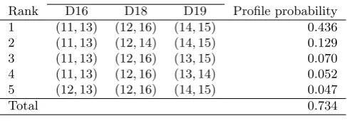
Table 4.Most probable genotypes of the unknown contributorUunder the hypoth-esisK1 &K2 &Uwhen information in the traces MC15 and MC18 is combined.
Marker
Rank D16 D18 D19 Profile probability
1 (11,13) (12,16) (14,15) 0.436
2 (11,13) (12,14) (14,15) 0.129
3 (11,13) (12,16) (13,15) 0.070
4 (11,13) (12,16) (13,14) 0.052
5 (12,13) (12,16) (14,15) 0.047
Total 0.734
We also note from Table 3 that the mixture proportionsφappear to be similar for the two traces, although the standard deviations indicate that they are not identical; indeed a likelihood ratio test for their identity is rejected under both hypotheses with p-values around 0.0003.
For curiosity we also analysed MC15 and MC18 using likeLTD obtaining a WoE of 8.8 bans. This number is not directly comparable to our analysis above as it refers to a slightly different database of allele frequencies and a coancestry parameter FST = 0.02 is applied together with a sampling adjustment, resulting in a larger match probability for
K3and thus a smaller maximal WoE of 13.2 bans. Furthermore,likeLTDassumes that the contributor fractions are identical for the two traces since they are treated as replicate runs of the same trace.
To compare with the analysis obtained by likeLTDwe have made an analysis with our model assuming equal contributor fractions, using the same database, sampling adjustment, and coancestry parameter. This correction can readily be made as it only involves appro-priate modification of the allele frequencies (Balding, 2013). Using a likelihood function based only on observed peak presence or absence, plugging in parameter estimates based on the observed peak heights, we get a WoE of 10.0 bans. The corresponding WoE based on observed peak heights is 12.7 bans. It seems fair to conclude that properly exploiting the information in peak heights gives a more efficient analysis of the traces than what can be obtained from allele classifications alone; this could be important for the analysis of mixtures more complex than those analysed here.
4.2. Mixture deconvolution
For mixture deconvolution we consider the traces jointly under the defence hypothesis modi-fied by removing one unknown contributor and identify the five most probable full genotypes of the unknown individualU. For most markers, these genotypes share that of the defen-dant K3; indeed the only variations are on markers D16, D18, and D19, where the most probable configurations are displayed in Table 4. The markers not represented in the table share the genotype of the defendant for all five most probable combinations. We note that the profile with the top rank is that of the defendant, and the evidence gives a probability to the unknown person having precisely this profile of 44%. The probability that the true profile of the unknown contributor is among the five genotypes listed is 73%.
is among the five most probable profiles is reduced to 1% and 39% compared to 73% for the traces combined. Also, for the single trace deconvolutions, the profile of the defendant is ranked fourth for both traces rather than first. Thus it is apparent that combining trace information for deconvolution purposes can be of considerable value as it gives a much clearer explanation of the samples.
4.3. Interpreting artefacts
Our model does not impose at the outset that a specific peak or allele is due to stutter, or has dropped out, or is silent. One of the features of DNAmixtures (Graversen, 2013) is to produce Bayesian networks for each marker with peak height evidence propagated. Thanks to the flexibility of Bayesian networks we can then elaborate these so as to explicitly represent artefacts.
We can also make simple modifications of the model to allow for the possible presence of silent alleles. In this way, we can answer queries like: what is the probability that an observed peak is due only to stutter? that a specific allele has dropped out? that an unknown contributor possesses a silent allele?
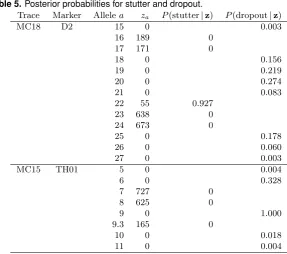
Identifying stutter and dropout To enable a precise analysis we shall say that an observed peak at a is due to stutter if no contributors possess allele a. Similarly we say that an alleleahasdropped out if at least one contributor possesses allelea, but no peak has been observed above threshold,i.e. Za= 0.
To investigate such events we introduce variablesYawhich explicitly represent the pres-ence or abspres-ence of the alleleaas follows
Ya=
(
1 ifP
inia>0
0 ifP
inia= 0.
These variables can readily be included in the network as nodes with parents nia and
probability propagation would then yieldP(Ya = 1|z) andP(Ya = 0|z). For an allele a
where a peak has been observed, the probability that the peak is due to stutter alone is now
P(stutter|z) =P(Ya = 0|z), whereas if no peak has been observed at a, the probability that the allelea has dropped out isP(dropout|z) = P(Ya = 1|z). A pre-classification of some alleles as, say, stutter or dropout corresponds to conditioning on specific values ofYa; the consequences of this conditioning can be obtained by a single probability propagation. A revised mixture analysis can then be performed conditionally on the pre-classification, should this be desired. We note that this form for preprocessing of data would still be consistent with our general model specification.
Table 5.Posterior probabilities for stutter and dropout.
Trace Marker Allelea za P(stutter|z) P(dropout|z)
MC18 D2 15 0 0.003
16 189 0
17 171 0
18 0 0.156
19 0 0.219
20 0 0.274
21 0 0.083
22 55 0.927
23 638 0
24 673 0
25 0 0.178
26 0 0.060
27 0 0.003
MC15 TH01 5 0 0.004
6 0 0.328
7 727 0
8 625 0
9 0 1.000
9.3 165 0
10 0 0.018
11 0 0.004
Unsurprisingly, the combined analysis of two traces gives more informative results on the analysis of artefacts than what emerges from separate analyses of the two traces. We refrain from reporting the separate analyses here.
Silent alleles The possibility that the unknown contributors might have a silent allele is incorporated in the model by adding an extra allelic type 0 (silent) to the genotype representations as displayed in Fig. 5. We now let ni0 ∼ Bin(2, q0), Si0 = ni0, Si1 =
ni1+Si0, and further ni1|Si0 ∼Bin(2−Si0, q1), where q0 is the probability of an allele being silent andq1 indicates the database allele frequency. Since no peak can be observed for the silent allele there is no observational node O0. This corresponds to a modification of the basic model where the allele frequencies qa, a > 0 are interpreted as the relative
Si1 Si2 Si3 Si4 Si5 Si6
ni1 ni2 ni3 ni4 ni5 ni6
O1 O2 O3 O4 O5 O6
Si0
ni0
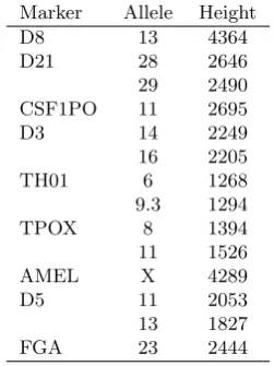
[image:25.490.128.361.508.594.2]Table 6. Excerpt of a DNA profile with peak heights of a single individual.
Marker Allele Height
D8 13 4364
D21 28 2646
29 2490
CSF1PO 11 2695
D3 14 2249
16 2205
TH01 6 1268
9.3 1294
TPOX 8 1394
11 1526
AMEL X 4289
D5 11 2053
13 1827
FGA 23 2444
frequencies of non-silent alleles, so the probability that a random allele is of typeais equal to (1−q0)qa ifa >0.
4.4. Single source analysis
Although our model is developed for the analysis of mixtures, it can also be useful in the analysis of a DNA profile from a single source; in particular as the peak heights can be informative about the presence of silent alleles. What appears to be a homozygous genotype at some marker may not be so; an alternative explanation is that we see only one allele of a heterozygous genotype, the other allele being silent. We would expect this to be reflected in a peak height that is smaller than expected and it will clearly affect the evidential interpretation of DNA profiles.
Table 6 shows an excerpt of a DNA profile of a single individual J, having apparent homozygous genotypes on markers D8, CSF1PO and FGA. Note that the peak heights are rather large, as is customary in single source data with a large amount of DNA.
Assuming that the DNA profile in Table 6 came from two unknown contributors and setting the threshold C = 50, we obtain estimates for the fraction of DNA from each unknown contributor of ( ˆφ1,φˆ2) = (1,0) which clearly indicate that the DNA trace comes from a single individual. The estimates of the other parameters are ˆµ= 1806, ˆσ= 0.290, ˆ
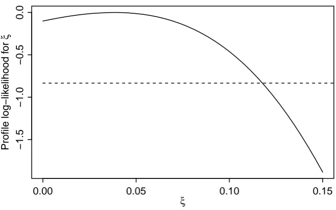
ξ = 0. The combination of a high mean peak height ˆµ = 1806 and a vanishing stutter proportion points to the data having been preprocessed so that peaks classified in the laboratory as stutter have been removed. If we instead set the threshold at C = 500 to ensure that the removed stutter peaks are well below threshold and assume that the data are from a single individual, we get the estimates ˆµ = 1854, ˆσ = 0.278 and ˆξ = 0.038. Clearly, there is very little information about the stutter proportion when stutter peaks have been removed, resulting in a very flat profile likelihood for the stutter proportion as shown in Fig. 6; indeed a 95% confidence interval forξwould be ranging from 0 to 11.8%.
0.00 0.05 0.10 0.15
−1.5
−1.0
−0.5
0.0
ξ
Profile log−lik
elihood f
or
[image:27.490.78.407.69.275.2]ξ
Fig. 6.Profile log-likelihoodmaxµ,σlog10L(µ, σ, ξ)−log10L(ˆµ,ˆσ,ξˆ)forξfor the single source trace
thresholded at C = 500. Values of ξ with log-likelihood above the horizontal line constitute an
approximate 95% confidence interval.
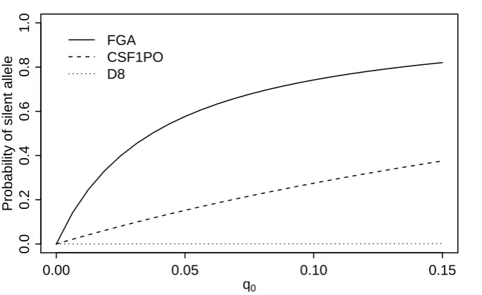
CSF1PO and FGA have peak heights around 60% and 56% that of D8, and correspondingly higher probabilities ofJ possessing a silent allele.
However, care should be taken with interpreting this result as FGA and CSF1PO often have a lower peak height than other markers, being at the end of the dye panel and thus corresponding to a longer fragment length, see also Section 5.2 below. Evidence calculations and deconvolutions may be less sensitive to this fact, but it could be of crucial importance for the identification of silent alleles.
5. Discussion
On the previous pages we have described a simple and versatile model for description of mixed DNA profiles and demonstrated how it could be applied to case analysis. We should emphasize that all our computations are direct consequences of our model and exact apart from the use of deterministic numerical optimization methods. Clearly, the model itself represents an approximation to reality, as any model will, but we believe it is a virtue that any further analysis — whether this be computation of likelihood ratios, deconvolution, or mixture interpretation — does not need additional approximations, modifications of the model, nor any ad hoc heuristics. Also, our method does not rely on a subjective pre-processing of the DNA profile with a manual or automatic system which identifies which alleles have been observed; such a pre-processing step constitutes an additional potential source of error.
0.00 0.05 0.10 0.15
0.0
0.2
0.4
0.6
0.8
1.0
q0
Probability of silent allele
[image:28.490.86.428.65.274.2]FGA CSF1PO D8
Fig. 7.Posterior probabilities that the individual has a silent allele as a function of the apriori
proba-bilityq0of having a silent allele.
proper case work. However, for any methodology there is room for improvement and below we shall briefly discuss some issues worthy of further attention.
We note in passing that the model could potentially also be useful in disputed paternity cases or other types of pedigree analysis where the DNA of some of the actors is available only in small quantities as in LTDNA, or is degraded.
5.1. Number of contributors
One issue is associated with determining the number of unknown contributors to the sample. The samples considered need at least three unknown contributors to be well explained. We have in the previous analyses introduced an additional unknown contributor to allow for spontaneous dropin, but showed that such an additional contributor had most likely only contributed tiny amounts of DNA to the mixture, if anything at all. Typically, a heuristic argument is used where additional contributors are not added unless they appeared to be necessary for explaining the DNA profile in question. However, Buckleton et al. (2007) and Biedermann et al. (2012) point out the risks in using this kind of approach.
As we operate with maximized likelihoods under hypotheses that there is at most a fixed number k of contributors, it is obvious that the maximized likelihood will increase — or at least not decrease — with the number of unknown contributors, both for the defence and prosecution. This follows from the fact that the hypothesis of at most k
0.0
0.1
0.2
0.3
0.4
Number of contributors
Change in bans
3 4 5 6 7 8
●
●
●
●
●
●
●
●
●
●
●
●
● ●
[image:29.490.81.406.72.279.2]Defence Prosecution WoE
Fig. 8. The maximized log-likelihood functions based on combining MC15 and MC18 for varying number of contributors and hypotheses, relative to their value for three contributors and displayed in bans.
ratio decreases with the number of contributors. The change is tiny: for eight contributors the WoE has decreased to 14 bans from 14.1 bans for three contributors, hardly of any significance. Even if the defence is allowed eight contributors and the prosecution stays with three, we get WoE = 13.7, which is still close to what would be obtained for a perfect match on nine markers and in most cases would imply identification ofK3as a contributor beyond reasonable doubt.
Inspection of the maximum likelihood estimates reveals that the five unknown contrib-utors associated with the smallest amount of DNA have between them supplied less than 3.7% of the total amount of DNA shared in equal proportions, i.e. each about 0.75% of the total amount of DNA. Bearing in mind that the total solution of DNA contains about 100 human cells, this means that effectively all of their alleles (which are not shared with the three major contributors or in stutter position to those) have not been observed. The presence of these unknown contributors just serves the purpose of explaining minor peak imbalances and seems irrelevant for the substantial interpretation of the mixture.
assumption that no allele has dropped out; the problem in our case is that one could have an infinite number of contributors with so little DNA that their alleles have only been observed through minor perturbations of the peak heights.
5.2. Extensions and modifications
The analyses presented in this paper have been made with the simplest possible variant of the model with sensible and rather robust results. However, there are some obvious potential improvements to be made.
Marker dependence of parameters We have assumed that the parameters (µ, σ, ξ) are iden-tical for all markers. This clearly contradicts findings in the literature (Butler, 2005; Puch-Solis et al., 2013) which indicate that both mean peak heights and stutter proportions depend on marker, fragment length, and may also be different for different dye panels in the EPG. Variation in these parameters can easily be incorporated in the model. However, as this could drastically increase the number of parameters, it would be best to do so by using prior information from laboratory experiments, for example by scaling peak heights as indicated in Puch-Solis et al. (2013) or by adding prior information by penalizing the likelihood function to ensure that parameter estimates are near those expected.
Degradation For strongly degraded DNA samples it is necessary to adjust the model by correcting for fragment length. From the analysis in Tvedebrink et al. (2012b) it seems that the simplest and most natural way to do so would be to assume the parameter ρ in the gamma distribution — being proportional to the amount of DNA — to depend exponentially on the fragment lengthλas
logρ=δλ+ζ.
This would just add one additional parameter δ representing the level of degradation of DNA to the model and would not in itself create specific difficulties for the methodology, although the complexity of the maximum likelihood estimation clearly increases whenever new parameters are added.
5.3. Other issues
Model criticism An important point that we have not touched upon in the previous analy-ses is the need to validate the model used for any given dataset. We find that it is not enough to compare the likelihoods for two competing hypothesis if neither of them can be demon-strated to give a plausible explanation of the data at hand. Promising graphical methods for systematic model validation and criticism based on its internal predictions and residual analysis are important and under development (Graversen and Lauritzen, 2013a). These methods exploit that the computational structure of a Bayesian network naturally enables fast prediction of peak heights based on partial information from the profiles. An example is given in Fig. 9 which shows the conditional probability transform of peak heights for MC15 and MC18 under the prosecution hypothesis against quantiles of the uniform distribution, indicating an excellent fit of the gamma model.
●●●●●● ●●●●●●●●● ●●● ●●●●●● ●●●●● ●●●●●●● ●●●●● ●●●●●●● ●●●●●●●●● ●●●●● ●●● ●●●●●●●●● ●●● ●●●●●● ●●●●●● ●●●● ●●●
0.0 0.2 0.4 0.6 0.8 1.0
[image:31.490.141.345.231.434.2]0.0 0.2 0.4 0.6 0.8 1.0 Uniform quantiles P( Za ≤ za | Zb = zb , b ≠ a , Za ≥ C ) ● ● MC15 MC18
Fig. 9. Conditional probability transform of observed peak heights for MC15 and MC18 vs. uniform quantiles.