Independent Factor Autoregressive Conditional Density Model

City, University of London Institutional Repository

Citation

: Urga, G., Ghalanos, A. & Rossi, E. (2015). Independent Factor Autoregressive

Conditional Density Model. Econometric Reviews, 34(5), pp. 594-616. doi:

10.1080/07474938.2013.808561

This is the accepted version of the paper.

This version of the publication may differ from the final published

version.

Permanent repository link:

http://openaccess.city.ac.uk/16373/

Link to published version

: http://dx.doi.org/10.1080/07474938.2013.808561

Copyright and reuse:

City Research Online aims to make research

outputs of City, University of London available to a wider audience.

Copyright and Moral Rights remain with the author(s) and/or copyright

holders. URLs from City Research Online may be freely distributed and

linked to.

Alexios Ghalanos ∗ Cass Business School, UK

Eduardo Rossi † University of Pavia, Italy Giovanni Urga‡

Cass Business School, UK and Bergamo University, Italy September 18, 2012

Abstract

In this paper, we propose a novel Independent Factor Autoregressive Conditional Density (IFACD) model able to generate time-varying higher moments using an independent factor setup. Our proposed framework incorporates dynamic estimation of higher comovements and feasible portfolio representation within a non elliptical multivariate distribution. We report an empirical application, using returns data from 14 MSCI equity index iShares for the period 1996 to 2011, and we show that the IFACD model provides superior VaR forecasts and portfolio allocations with respect to the CHICAGO and DCC models.

Keywords: Independent Factor Model, GO-GARCH, Independent Component Analysis, Time-varying Co-moments.

JEL Classification: C13, C16, C32, G11.

Abstract

In this paper, we propose a novel Independent Factor Autoregressive Conditional Density (IFACD) model able to generate time-varying higher moments using an independent factor setup. Our proposed framework incorporates dynamic estimation of higher comovements and feasible portfolio representation within a non elliptical multivariate distribution. We report an empirical application, using returns data from 14 MSCI equity index iShares for the period 1996 to 2011, and we show that the IFACD model provides superior VaR forecasts and portfolio allocations with respect to the CHICAGO and DCC models.

Keywords: Independent Factor Model, GO-GARCH, Independent Component Analysis, Time-varying Co-moments.

1

INTRODUCTION

This paper develops an independent factor model for the conditional density of financial returns with

time-varying skewness and kurtosis. In the presence of nonnormally distributed asset returns, optimal

portfolio selection techniques require estimates of variance-covariance parameters, along with estimates

of higher-order moments and co-moments of returns. The importance in portfolio analysis of modelling

higher conditional moment dynamics has been highlighted by, inter alia, Barone Adesi et al. (2004),

Beaulieu et al. (2007, 2009), Chabi-Yo et al. (2008), Harvey and Siddique (1999), Martellini and

Ziemann (2010), Mencia and Sentana (2009, 2012), Sentana (2009), and Wilhelmsson (2009). In the

univariate context, models that include higher moments dynamics have received growing attention.

See for example Jondeau and Rockinger (2003, 2009), Harvey and Siddique (1999), Rockinger and

Jondeau (2002), and Wilhelmsson (2009). However, little effort has been devoted to incorporate such

dynamics in a multivariate context, mainly because of the difficulty to parameterize marginal and

joint distributional parameters. There are very few notable exceptions. Mencia and Sentana (2009)

adopt a flexible family of multivariate asymmetric distributions, known as location-scale mixtures of

normals, which nests as particular cases several important elliptical symmetric distributions. When the

distribution of asset returns can be expressed as a location-scale mixtures of normals, then the portfolio

conditional distribution has time-varying higher moments arising from the interaction of the dynamics

of the location, scale and skew parameters. On the other hand, Jondeau and Rockinger (2009) propose

an asymmetric DCC-skew-T model with higher moment dynamics, but the presence of the skew and

shape parameters in the conditional likelihood makes the estimation feasible only for a few assets.

Broda and Paolella (2009) propose a Conditionally Heteroskedastic Independent Component Analysis

of Generalized Orthogonal GARCH of van der Weide (2002), the CHICAGO model, which is based

on a multivariate affine representation of the Normal Inverse Gaussian (maNIG), originally proposed

by Schmidt et al. (2006). In the CHICAGO model higher moments of the conditional distribution

of asset returns are explicitly modelled albeit they are constant. The estimation of the CHICAGO

model is based on the Independent Components Analysis (ICA) method used in Chen et al. (2008)

and Zhang and Chan (2009). Unlike other models, independence offers a greater deal of flexibility

in modelling the full marginal dynamics within a multivariate affine factor framework, enabling the

calculation of conditional portfolio density used in risk management applications.

which extends the CHICAGO model by allowing for a flexible parametrization of the dynamics of factor

higher moments. The marginal density of each independent factor is supposed to be a one-dimensional

Generalized Hyperbolic (GH) distribution, with skew and shape parameters modelled with

autoregres-sive dynamics, as in the Autoregresautoregres-sive Conditional Density (ACD) model of Hansen (1994). This

entails that the conditional density of returns is the multivariate affine GH (maGH) of Schmidt et al.

(2006). An interesting implication of this factor representation is that conditional higher moments of

asset returns and portfolios have a closed-form expression, and the portfolio conditional density can

be obtained by Fast Fourier Transform (FFT).

The paper is organized as follows. Section 2 introduces the IFACD model. In Section 3, we

introduce the conditional maGH distribution with higher moments dynamics. Key features such as

the conditional higher comoment tensors are presented in Section 4, where we also propose a portfolio

conditional density representation. The estimation of the model and the ICA algorithm are outlined

in Section 5, where we report the results of a risk and portfolio management application, comparing

IFACD to CHICAGO and DCC(T) models, using a representative dataset of international equity

indices spanning the last two decades. Section 6 concludes. In Appendices A and B, we details the

GH density and its characteristic function.

2

THE INDEPENDENT FACTOR MODEL

Factor ARCH models, originally introduced by Engle et al. (1990) and with foundations in the

Arbi-trage Pricing Theory of Ross (1976), are based on the assumption that returns are generated by a set

of unobserved underlying factors that are conditionally heteroscedastic. The dependence framework

is static as a consequence of large scale estimation in a multivariate setting. Consider a set of N

assets whose returns rt are observed for T periods, with conditional mean E[rt|Ft−1] = mt, where

Ft−1 is the σ-field generated by the past realizations of rt, i.e. Ft−1 =σ(rt−1,rt−2, . . .). The

Gener-alized Orthogonal GARCH (GO-GARCH) model of van der Weide (2002) mapsrt−mt onto a set of

unobserved independent factorf_t (or ”structural errors”)

rt = mt+ǫt t= 1, . . . , T (1)

where A is invertible and constant over time and may be decomposed into the de-whitening Σ1/2,

representing the square root of the unconditional covariance matrix, and orthogonal matrix,U

A=Σ1/2U, (3)

and f_t= (f1t, . . . , fN t)′. In this model it is assumed that the factors have the following specification

f_t=H1/2_t zt (4)

whereHt=E[ftf′t|Ft−1] is a diagonal matrix with elements (h1t, . . . , hN t) which are the conditional

variances of the factors, andz_t= (z1t, . . . , zN t)′. The random variablezitis independent ofzjt−s∀j6=i

and _∀s, with E[zit|Ft−1] = 0 and E[z2_it] = 1, this implies that E[ft|Ft−1] = 0 and E[ǫt|Ft−1] = 0.

The factor conditional variances,hi,t, can be modelled as a GARCH-type process. The unconditional

distribution of the factors is characterized by

E[f_t] =0 E[f_tf′_t] =IN (5)

which, in turn, implies that

E[ǫt] =0 E[ǫtǫ′t] =AA′. (6)

It follows that the returns can be expressed as

rt=mt+AH1/2t zt. (7)

The conditional covariance matrix,Σt≡E[(rt−mt)(rt−mt)′|Ft−1] of the returns is given by

Σt=AHtA′. (8)

The estimation of GO-GARCH by maximum likelihood suffers severely from dimensionality issues.

Alternative approaches such as nonlinear least squares and method of moments for the estimation of

U have been proposed in Boswijk and van der Weide (2006, 2011). In this paper, we estimate theU by

ICA as in Broda and Paolella (2009) and Zhang and Chan (2009). One of the computational advantages

factors, the dynamics of the marginal density parameters of those factors may be estimated separately.

In this context, we propose to extend the dynamics to the full conditional density parameters to

model in a multivariate setting time-varying higher moments. We consider the dynamics of the

independent factors in the context of an expanded GO-GARCH model with dynamics for the full

conditional parameters. While any multivariate distribution, admitting an affine representation may

be used in this setup, we choose the GH distribution of Barndorff-Nielsen (1977), in the multivariate

affine representation introduced by Schmidt et al. (2006), for its flexibility and rich parametrization,

capturing some of the most important features of observed returns such as asymmetry and fat tails.

3

AUTOREGRESSIVE CONDITIONAL GH DISTRIBUTION

The GH distribution is a variance-mean mixture of normal and Generalized Inverse Gaussian (GIG)

distributions. It is a flexible distribution, allowing for skewness and fat tails, nesting a large number of

distributions such as the Hyperbolic, Normal Inverse Gaussian, Variance Gamma, skew-Laplace, and

as limiting cases, the Normal and skew-T distributions. Then-dimensional GH distribution allows for

different marginal skewness. However, Schmidt et al. (2006) point out that the margins of a random

vector that is GH distributed are not mutually independent for some choice of the scaling matrix.

As a consequence, they propose an alternative, non-elliptical, maGH distribution with independent

margins allowed to take separate values for skewness and shape. See also Ferreira and Steel (2006) for

a multivariate skew-T density with independent margins.

Based on the parametrization of Schmidt et al. (2006), the vector of returnsr_t, which is expressed

as a linear transformation of independent factorsf_t∈RN as in (7), is conditionally maGH distributed

rt|Ft−1∼maGHN(mt,Σt,ωt), (9)

where ω_t = (ω1t, . . . , ωN t)′ and ωit = (λi, αit, βit)′ represent the time-varing conditional shape and

skew parameter vectors, respectively. In the IFACD model we assume that the standardized random

variables zit are conditionally distributed as a standardized GH. In general, the GH density of the

random variableY is given by

gh(y;λ, µ, δ, α, β,) =

K_λ−1/2αpδ2_{+ (y−µ)}2_eβ(y−µ)

where

c= α

2_−β2λ/2

√

2παλ−1/2_δλ_K λ

δpα2_−β2.

Alternative distributions are nested in (10), e.g. the NIG distribution is obtained by settingλ=₋1₂,

the Hyperbolic with λ = n+1₂ , and the skew-Student by setting λ = ₋ν₂ (with ν representing the

degrees of freedom) and α _{→ |}β_|, where parameters β and α are the skewn and shape parameters

of the distribution, respectively. A number of location and scale invariant parameterizations of the

GH distribution have been proposed in the literature. For the standardized GH distribution of zit we

choose the location scale invariant representation (ρ, ζ) because we are interested in ACD modelling

of skewness and kurtosis,

ζ =δpα2_−β2_{, ρ=} β

α. (11)

The relation between the parameters (ρ, ζ) and (α, β, δ, µ) and the standardization of the GH random

variable are detailed in Appendix 6. The skew and shape parameters (ρ, ζ) jointly determine the

skewness and kurtosis (Appendix 6 reports the expressions of skewness and kurtosis of the NIG

distribution). Bl¨aesild (1981) proved that a linear transformation such asaX+bof a random variable

X following a GH distribution in (10) is GH distributed with parameters λ∗ _{= λ, α}∗ _{= α/|a|,}

β∗ _{= β/|a|, δ}∗ _{= δ|a|, and µ}∗ _{= aµ +b. The choice of alternative parameterizations involves}

the appropriate transformation. Given (4), the single factors, fit, i = 1, . . . , N, are conditionally

distributed as agh(fit;λi, µit√hit, δit√hit, αit/√hit, βit/√hit).

We now turn to the specification of the time-varying skew and shape parameters. We adopt

a quadratic dynamics for the skew parameter (˘ρi,t) and a piece-wise linear dynamics for the shape

parameter (˘ζi,t)

˘

ρit=χ0i+χ1iκ1izit−1+χ2iz2it−1+ξ1iρ˘it−1

˘

ζit=κ0i+κ1izit−11[zit−1<−1]+κ2izt−11[zit−1>1]+ψ1iζ˘it−1,

(12)

where1is the indicator function such that positive (negative) standardized innovations, larger (smaller)

than one standard deviation, have a different impact on the skew dynamics. In this way the shape

responds only to shocks larger (or smaller) than one conditional standard deviation, because shocks

transform is then used to map the unconstrained processes ˘ρi,t and ˘ζi,t intoρi,t and ζi,t:

ρit =−0.99 +

1.98

1 +e−ρ˘it (13)

ζit = 0.1 +

24.9 1 +e−ζ˘it

(14)

where the bounds of the distributional parameters are [₋0.99,0.99] and [0.1,25] for ρ and ζ, respec-tively. We limit the upper bound ofζ to 25, since values beyond this point lead to very little change in the skewness and kurtosis, with the range 0.1 to 25 representing most of the cases, whereas the bounds

for ρ are simply dictated by the GH distribution. In theory, the GIG shape parameter λi is allowed

to vary for each factor, but this introduces an added layer of complexity since different combinations

of λ,ρ and ζ lead to the same or close likelihood. Alternatively, choosing a value ofλequal to ₋0.5, which corresponds to the NIG distribution, we have enough flexibility to account for the observed

non-Gaussian features of financial time series. This is our choice in the empirical implementation of

IFACD model in Section 5.

In the next section, we present the conditional co-moments and portfolio conditional density

im-plied by the IFACD model, employed in the approximation of the expected utility in Section 5.4.

4

CONDITIONAL CO-MOMENTS AND

PORTFOLIO CONDITIONAL DENSITY

The novelty of the IFACD model is that the co-moments are now time-varying, as a consequence of

the ACD specification of the conditional density of the standardized innovations. The conditional

co-moments ofrt of order 3 and 4 are represented as tensor matrices

M3_t =A′M3_f,t(A_⊗A), M4_t =A′M4_f,t(A_⊗A_⊗A), (15)

where M3_f,t and M4_f,t are the (N _×N2_{) conditional third comoment matrix and the (N ×N}3₎

conditional fourth comoment matrix of the factors, respectively. M3_f,t and M4_f,t, are defined as

M3_f,t =

M3_1,f,t,M3_2,f,t, . . . ,M3_N,f,t

(16)

M4_f,t =

M4_11,f,t,M4_12,f,t, . . . ,M4_1N,f,t|. . ._|M4_N1,f,t,M4_N2,f,t, . . . ,M4_{N N,f,t}

where M3_k,f,t, k = 1, . . . , N and M4_kl,f,t, k, l = 1, . . . , N are the (N _×N) submatrices of M3_f,t and

M4_f,t, respectively, with elements

m3_ijk,f,t = E[fi,tfj,tfk,t|Ft−1]

m4_ijkl,f,t = E[fi,tfj,tfk,tfl,t|Ft−1].

Since the factorsfitcan be decomposed aszit√hit, and given the assumptions onzit, thenE[fi,tfj,tfk,t|Ft−1] =

0. It is also true that fori₆=j₆=k₆=l,E[fi,tfj,tfk,tfl,t|Ft−1] = 0 and wheni=j and k=l

E[fi,tfj,tfk,tfl,t|Ft−1] =hithkt.

Thus, under the assumption of mutual independence, all elements in the conditional co-moments

matrices with at least 3 different indices are zero. Finally, we standardize the conditional co-moments

to obtain conditional coskewness and cokurtosis of rt

Sijk,t=

m3_ijk,t

(σi,tσj,tσk,t)

, Kijkl,t=

m4_ijkl,t

(σi,tσj,tσk,tσl,t)

, (18)

where Sijk,t represents the coskewness between elements i, j, k of rt, σi,t the standard deviation of

r_i,t, and in the case of i = j =k represents the skewness of asset i at time t, and similarly for the cokurtosis tensorK_ijkl,t.1

An important question that can be addressed in this framework is the determination of the portfolio

conditional density, an issue of vital importance in the risk management application. Let Rt be the

portfolio return

Rt=w′trt=w′tmt+ (w′tAH1/2t )zt (19)

whereH1/2_t is obtained from the ACD dynamics of estimated f_t. The portfolio conditional variance,

1_{A natural application of return co-moments matrices is the news impact surface (as first suggested by Kroner and}

skewness and kurtosis in closed form are

σ2_R,t=w′_tΣtwt,

sR,t=

w′_tM3_t(wt⊗wt)

(w′

tΣtwt)3/2

,

kR,t=

w′_tM4_t(wt⊗wt⊗wt)

(w′

tΣtwt)2

,

(20)

where Σt, M3t and M4t are derived in (8) and (15), respectively. The portfolio conditional density

may be obtained via the inversion of the characteristic function through the FFT method as in

Chen et al. (2007) (see Appendix 6 for details) or by simulation. We implement the FFT for its

accuracy and speed. While theN-dimensional NIG distribution is closed under convolution, when the

distributional parameters α and β are allowed to be different across assets, as in the case of IFACD

model, this property no longer holds. Provided that z_t is a N-dimensional vector of innovations,

marginally distributed as 1-dimensional standardized GH, the density of weighted asset return,witrit,

is

wi,tri,t= (wi,tmi,t+wi,tzi,t)∼maGH1

wi,tµi,t+wi,tmi,t,|wi,t|δi,t, λi,

αi,t

|wi,t|

, βi,t

|wi,t|

(21)

where w′_t is equal to w′_tAH1/2_t , and wi,t is the i-th element of wt,mi,t the conditional mean of the

i-th underlying asset. In order to obtain the density of the portfolio, we must sum the individual

weighted densities ofzi,t. The characteristic function of the portfolio return Rt is

ϕR(u) = n

Y

i=1

ϕwZ¯ i(u) = exp

 iu

d

X

j=1

¯

µj+ d X j=1 λj 2 log _γ υ

+ log Kλj(¯δj

√

υ)

Kλj(¯δj

√_γ)

!!

 (22)

where, γ = ¯α2

j−β¯j2,υ= ¯α2j−( ¯βj+ iu)2, and (¯αj,β¯j,¯δj,µ¯j) are the scaled versions of the parameters

(α, βi, δi, µi) as shown in (21). The density is accurately approximated by FFT as follows

fR(r) =

1 2π

Z +∞

−∞

e(−iur)ϕR(u)du≈

1 2π

Z s

−s

e(−iur)ϕR(u)du. (23)

Expression (23) is the base for the calculation of VaR in the empirical application reported in Section

5

EMPIRICAL APPLICATION

In this section, we report results of an empirical exercise using data on 14 MSCI Global Equity indices

representing a cross section of countries in North America (U.S., Canada, Mexico), Asia (Australia,

Hong Kong, Japan, Singapore) and Europe (Germany, France, Spain, Italy, U.K., Switzerland,

Swe-den), from 12/08/1996 to 28/12/2011, and obtained from Yahoo Finance. The period includes the

Asian Financial Crisis of 1997, the Russian Financial Crisis of 1998, the Dot-Com bubble of 2000 and

subsequent economic downturn of 2002, the Chinese Stock Bubble of 2007, the US Bear Market of

2007-2009, the European sovereign debt crisis of 2010 as well as the flash crash of May 2010.2 First,

we report (Section 5.2) an in-sample comparison of the IFACD and CHICAGO models in order to

obtain some insight into the types of dynamics and parametrization of the factors. In Section 5.3, we

report the results of an out-of-sample risk forecast evaluation using randomly weighted portfolios to

avoid any bias arising from the uncertainty in selecting any particular set of weights. In Section 5.4,

a Taylor series expansion of the Constant Absolute Risk Aversion (CARA) utility function is used for

an out-of-sample portfolio allocation to contrast the time-varying versus the static representation of

higher conditional co-moment matrices.

In the following subsection, we briefly describe the ICA method, used to estimate the independent

factors, and we introduce the likelihood function.

5.1 Estimation Procedure

The estimation procedure of the IFACD model can be summarized as follows. First, we compute the

ICA of the dataz_t=Σb−1/2bǫ_t, wherebǫ_tare the OLS residuals, i.e. bǫ_t=r_t−cm_t, andΣb1/2 is obtained from the eigenvalue decomposition of the OLS residual covariance matrix. ICA provides an estimate of

the orthogonal matrixU in (3) as in Broda and Paolella (2009) and Zhang and Chan (2009). The ICA

is a computational method for separating multivariate mixed signals, x = [x1, ..., xn]′, into additive

statistically independent and non-Gaussian components,s= [s1, ..., sn]′, such that x=Bs. The

esti-mate of the linear mixing matrixB can be obtained via the algorithm, proposed and implemented by

Hyv¨arinen and Oja (2000). The FastICA algorithm is based on negentropy, which is an optimal

esti-mate of non-Gaussianity, as shown by Comon (1994), is invariant to invertible linear transformations.

Thus the estimatedf_tare obtained as ˆf_t=Σb−1/2U zb t. Second, because of the assumption of

indepen-2_{The tickers of these iShare tradeable indices, in the order presented are: SPY, EWC, EWW, EWA, EWH, EWJ,}

dence, the likelihood function of the IFACD model is greatly simplified. The conditional log-likelihood

function is expressed as the sum of the individual conditional log-likelihoods, derived from the

condi-tional marginal densities of the factors, i.e., gh( ˆfit) ≡gh( ˆfit;λi, µit√hit, δit√hit, αit/√hit, βit/√hit),

plus a term for the mixing matrix A, estimated in the first step by FastICA

L(_bǫt|θ,A) =Tlog

A−1+

T

X

t=1 N

X

i=1

loggh( ˆfit|θi)

(24)

whereθis the vector of unknown parameters in the marginal densities. The possibility of modelling the

independent factors separately not only increases the flexibility of the model but also its computational

feasibility, since the multivariate estimation reduces to N univariate optimization steps plus a term

which depends on the factor loading matrix.

5.2 In-sample Estimation

In Table 1, we report the results of the first in-sample fit of the IFACD and CHICAGO models for the

period 19/03/1996 to 17/03/2000, in order to illustrate the factors’ dynamics and their significance.

The CHICAGO model consists of (1)-(8), but with the conditional distribution of fit which has only

the second moment time-varying and constant higher moments, and the matrixU in (3) estimated by

FastICA. Both models are estimated under the maNIG distribution. Because of the presence of first

degree autocorrelation in the MSCI index dataset, the returns were demeaned and filtered with an

AR(1) model prior to applying the FastICA algorithm. In both models, the factor variance dynamics

follow a GARCH(1,1) model with parameters (ω, α1, β1), and in the IFACD the skew and shape

dynamics follow a first order quadratic and piece-wise linear model with parameters (χ0, χ1, χ2, ξ1)

and (κ0, κ1, κ2, ψ1) respectively, as in (12). Given that ICA is conceived as a linear noiseless model, the

standard errors are computed only in the estimation of the factors’ conditional distribution parameters.

Starting with the CHICAGO model, the very small absolute value and lack of significance of

the skew parameter ρ indicates that skewness is not very pronounced in this sample, and the skew

dynamics of the IFACD model somewhat bear this out since very few factors appear to have significant

skew dynamics. The same cannot be said of the shape parameterζ which is significant in the majority

of factors and varies between 1.7 and 2.5, with the exception of Factor 10 which does not appear

to have significant skew or shape, and in combination with a zero skew parameter translates to an

majority of the factors in the IFACD model. With regard to the variance dynamics, they appear to be

the same across the two models, though there is some evidence from Factors 1, 12 and 14 that when

persistence is very high in the CHICAGO model, the IFACD model persistence instead is much lower

as the shape dynamics accommodate expansions and contractions in the conditional density shape

which would otherwise be completely captured by the GARCH variance dynamics. Finally, while the

factor log-likelihoods (and hence model log-likelihood) of the IFACD model are always higher than

those of the CHICAGO model, the higher BIC of the former indicates that there is a small penalty

for the overparametrization.

5.3 Out-of-sample Risk Forecast

The out-of-sample comparison is based on one-step ahead forecasts. We estimate the models every

five days, keeping a constant sample size, for a total of 522 re-estimations resulting in 2610 forecasts.

Starting from 17/03/2000, the last 4 years of daily log returns are used to estimate IFACD models, CHICAGO, and DCC(T). In order to evaluate the contribution that the ACD specification gives to

the model’s performance, in addition to the IFACD model with the time-varyingρtandζt, we consider

two restricted versions of the model which have constant skew and time-varying shape, i.e. (ρ, ζt), and

time-varying skew and constant shape, i.e. (ρt, ζ), respectively. We also include the DCC(T) model so

as to gauge the cost of IFACD which is based on unconditional independence. The model is specified

and estimated as in Bauwens and Laurent (2005).

The consistency between the IFACD and CHICAGO models was guaranteed by using the same

mixing matrixAacross the two models for each estimation window so that the only difference is purely

in the dynamics of the factors. Because of the non-dynamic nature of the mixing matrix in the IFACD

model, the rolling window re-estimation scheme with a fixed size of 4 years enables to capture any

change to the loadings, though tracking such changes is not trivial since the independent components

are identified only up to a permutation and scaling of the sources. To evaluate the forecast performance

of the models, a weighted linear combination of the forecast density was used in order to form portfolios

from which measures could easily be calculated. To avoid bias from any particular weighting scheme,

1000 + 1 random portfolios are generated by sampling weights from the exponential distribution (the

1001th _{is the equally weighted portfolio) and dividing by the sum of the randomly generated deviates}

to create the full investment constraint. The weighted densities of the IFACD and CHICAGO models

functions are easily created. For DCC(T) model the portfolio moments used to compute functions of

the density are obtained using the standard linear and quadratic transformations of the forecast mean

and covariance matrix. The following tests are used to evaluate the forecasting accuracy of the risk

models: Berkowitz (2001) for testing the predictive density, Kupiec (1995) and Christoffersen (1998)

for VaR exceedances, and Christoffersen and Pelletier (2004) for VaR Durations.

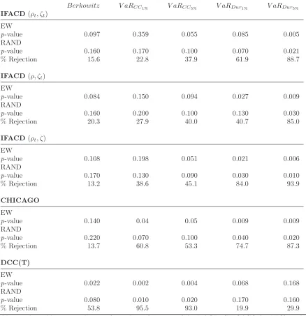
Table 2 reports the result under the different tests for the equally weighted (EW) and average of

the randomly weighted (RAND) portfolios. For the Berkowitz test, there is no significant difference

between the factor models, with a rejection rate among the randomly weighted portfolios of about 16%

and 14% for the IFACD(ρt, ζt) and CHICAGO models respectively, indicating that overall both models

fit the out-of-sample forecast density well. The same is true for the IFACD models with constrained

ACD dynamics. The DCC(T) model on the other hand does not fit the conditional weighted forecast

densities very well, with more than 50% rejection rate.

For the VaR tests, both at the 1% and 5% coverage rates, the IFACD(ρt, ζt) model performs better

than the other two IFACD models and the CHICAGO, as evidenced by the large difference in rejection

rates. In the VaR Duration test with 1% coverage, the IFACD(ρt, ζt) and IFACD(ρ, ζt) dominate the

CHICAGO. However, the DCC(T) outperforms the factor models and this is indicative of the value of

dynamic correlation since the duration indirectly tests for clustering of tail events which is not likely

to be fully filtered out in a static independent factor framework.

5.4 Out-of-sample Optimal Portfolio Forecast

We consider an alternative approach to the standard quadratic model of Markowitz (1952) is based

on the approximation of the utility function via a Taylor series expansion. In each period, an investor

allocates capital to maximize the conditional expected utility, Et−1[U(Wt)], over the next period

wealthWt, with initial wealth equal to 1. The optimal allocation problem may be formulated as:

max

wt

Et−1[U(Wt)], s.t. N

X

i=1

wti= 1, wti>0 ∀i, (25)

where we assume the absence of a riskless asset, so that the sum of the weights wti sums to one;

we also exclude the possibility of short-selling. The expected utility can be written, using a Taylor

(2006)), as

Et−1[U(W)] =U W¯t+U(1) W¯tEt−1Wt−W¯t+

1 2U

(2) _W¯ tEt−1

h

Wt−W¯t2

i

+1

3U

(3) _W¯ t

Et−1

h

Wt−W¯t

3i

+1

4U

(4) _W¯ t

Et−1

h

Wt−W¯t

4i

+O W_t4, (26)

where ¯Wt=w′tEt−1[rt] is the expected portfolio return and O Wt4

represents the remainder of the

Taylor series due to the truncation.

Note that this approximation includes two moments more than the mean-variance criterion, with

the skewness and kurtosis are directly related to investor preferences (dislike) for odd (even) moments,

under certain mild assumptions given in Scott and Horvath (1980). The expected utility can then be

approximated as

Et−1[U(Wt)]≈U W¯t

+1

2U

(2) _W¯ t

σ_R,t2 + 1 3!U

(3) _W¯ t

˜

sR,t+

1 4!U

(4) _W¯ t

_˜

kR,t. (27)

where ˜sR,t ≡ Et−1

h

Wt−W¯t3

i

and ˜kR,t ≡ Et−1

h

Wt−W¯t4

i

are the nonstandardized versions of

conditional skewness and kurtosis, namely the numerators in (20). When the CARA utility function

is used, then the approximation resolves to:

Et−1[U(Wt)] =Et−1[−exp (−ηWt)]≈ −exp −ηW¯t

1 +η

2σ

2 R,t−

η3

3!s˜R,t+

η4

4!˜kR,t

, (28)

whereηrepresents the investor’s constant absolute risk aversion, with higher (lower) values represent-ing higher (lower) aversion. It is evident from (28) that the conditional kurtosis has a negative impact

on the expected utility while the positive conditional skewness has a positive one. We maximize this

function for all rolling forecasts using a nonlinear Sequential Quadratic Programming solver and

mak-ing use of the first order derivatives given in Jondeau and Rockmak-inger (2006). Upper bounds (50%) are

imposed on the assets weights.

Table 3 shows the results for the IFACD, CHICAGO and DCC models of CARA utility portfolios

maximized under 4 different risk aversion coefficients from the mildly risk averse to extremely risk

averse investor. The results of this exercise confirm the benefit of considering higher conditional

moments in portfolio allocation. As the risk aversion coefficient increases, and consequently more

weight is given to the higher moments in the conditional expected utility, the IFACD(ρt, ζt) model

model confidence set (MCS) of Hansen et al. (2011), using as loss function the negative of the portfolio

returns, which overwhelmingly rejects both the CHICAGO and DCC(T) models fromη= 10 onwards,

with 90% confidence.

Turning to IFACD models with constrained ACD dynamics, we have very similar results to those

of IFACD(ρt, ζt). This can be explained by the fact that both the skew and shape parameters jointly

determine the tail behavior in the NIG/GH distribution, so that when there is very little variation in

the conditional asymmetry, as in our sample, the skew parameter is mostly adjusting to compensate

for the fixed shape parameter in determining the dynamics in the tail behavior. The portfolios based

on IFACD models underweight securities with high predicted kurtosis and negative skewness, and as

a result, when η increases and more emphasis is placed on higher moments, the average return and

Risk-Reward (RR) ratio, in Table 3, are significantly higher than the CHICAGO and DCC(T) models.

A slow progression is seen when it comes to the significance of RR differences given by the test of

Ledoit and Wolf (2008), with the IFACD(ρt, ζt) model RR ratio significantly better at η = 25 with

90% confidence. Not surprisingly, the DCC model based on the CARA utility expansion with only 3

moments fares worse at all levels of risk aversion.

6

CONCLUSIONS

In portfolio and risk management analysis, it is important to consider not only asymmetric and

heavy tailed multivariate distributions but also time-varying skewness and kurtosis. Modelling the

conditional density dynamics in a multivariate setup has proved unfeasible mainly because of the

difficulty in dealing with tractable representations of non-elliptical multivariate distributions. In this

paper, we propose the IFACD model where the returns have a maGH distribution with time-varying

higher moments. These features allow us to model extreme behaviors of financial markets turmoils.

The IFACD model uses time-varying distributional parameters in a multivariate setting, for truly

large scale models. Further, the IFACD model has closed form higher moments and semi-analytic

expression for the portfolio density which have important implications for portfolio allocation and risk

management analysis. Modelling higher moments as a time-varying processes is highly appropriate

for periods of market stress, when GARCH models cannot accommodate extreme events. We report

evidence of this via large out-of-sample risk management and portfolio applications: using 14 MSCI

CHICAGO and DCC(T) models.

The findings in this paper suggest further developments. For instance, it would be interesting to

study consistent procedures able to provide more parsimonious independent factor representations.

Further, the use of IFACD model with high-frequency data or realized measures would be a useful

extension to mimic the evolution of volatilities in real time. We leave these issues to future research.

ACKNOWLEDGEMENT

This work started while the second author was visiting the Centre for Econometric Analysis at Cass

Business School in summer-fall 2009. We thank participants in the 4th CSDA International Conference

on Computational and Financial Econometrics (London, 10-12 December 2010), the Fourth Italian

Congress of Econometrics and Empirical Economics (Pisa, 19-21 January 2011). We wish to thank the

Editor, Esfandiar Maasoumi, an Associate Editor and two anonymous referees for useful comments

A

.

G

h

a

la

n

o

s

e

t

a

l.

IFACD Factors

f1 f2 f3 f4 f5 f6 f7 f8 f9 f10 f11 f12 f13 f14

ω 0.228*** 0.012 0.056 0.012 0.067* 0.012 0.059 0.040 0.085 0.054*** 0.018*** 0.203*** 0.430*** 0.139**

α1 0.090*** 0.055** 0.087 0.021 0.079*** 0.017 0.114 0.067 0.064 0.054*** 0.037*** 0.071 0.290 0.038*** β1 0.691*** 0.935*** 0.869*** 0.969 0.850*** 0.972** 0.832*** 0.888*** 0.846*** 0.898*** 0.946*** 0.731*** 0.350** 0.820*** χ0 0.077* -0.090 0.029 0.284 -0.277** 0.218 0.031 -0.230 0.028** -0.025 -0.036 0.061 0.056 -0.173 χ1 0.145** 0.133 0.234*** -0.286 0.008 0.050 0.125 0.303* 0.042 0.783** 0.193 0.109 0.227* 0.568 χ2 -0.068* -0.039 -0.061 -0.206 0.071* -0.178 -0.018 0.117 -0.025** -0.089 0.092 -0.020 0.012 0.382 ξ1 0.921*** 0.210 0.719 0.002 0.000 0.009 0.895*** 0.392* 0.929*** 0.438** 0.007 0.000 0.585 0.246 κ0 -2.373 -2.408*** -0.135 -1.096 -0.255* -2.317 -0.015 -0.010 -2.791*** 0.320 -1.614* 0.246 -2.273 -2.365*** κ1 0.489** 0.244 0.223*** 0.449 -0.392** 0.453 0.380 -0.052 0.479 0.174 -0.746 0.572* 0.681 -0.247 κ2 -0.943*** -0.045 -0.633*** -0.474 0.089 -0.289 -0.512*** -0.132 0.955* -1.000 0.981 -0.999 -0.998*** 1.000 ψ1 0.001 0.000 0.882*** 0.425 0.941*** 0.000 0.911*** 0.986*** 0.008 0.957*** 0.403 0.889*** 0.001 0.000

α1+β1 0.781 0.990 0.956 0.989 0.929 0.989 0.946 0.955 0.911 0.951 0.983 0.802 0.641 0.858

F actorLL -1391.15 -1356.72 -1362.39 -1400.23 -1353.69 -1397.26 -1327.67 -1342.91 -1346.19 -1418.20 -1384.97 -1416.16 -1373.69 -1383.06

F actorBIC 2.83 2.76 2.78 2.85 2.76 2.85 2.71 2.74 2.74 2.89 2.82 2.88 2.80 2.82

M odelLL 41148

M odelAIC -5.80

M odelBIC -5.72

CHICAGO Factors

f1 f2 f3 f4 f5 f6 f7 f8 f9 f10 f11 f12 f13 f14

ω 0.044* 0.010 0.039 0.015 0.069* 0.012 0.081** 0.046** 0.063** 0.057 0.025 0.001 0.299* 0.004

α1 0.031* 0.050*** 0.045** 0.019** 0.096*** 0.018* 0.086** 0.070*** 0.060*** 0.052* 0.042** 0.000 0.135** 0.001 β1 0.926*** 0.942*** 0.915*** 0.967*** 0.835*** 0.971*** 0.826*** 0.883*** 0.873*** 0.893*** 0.934*** 0.999*** 0.561** 0.995*** ρ 0.071 -0.088 -0.102 0.065 -0.108* 0.010 0.048 -0.098 0.031 -0.011 0.009 0.007 0.086 0.005

ζ 1.781*** 1.944*** 1.840*** 2.343*** 1.781*** 1.832*** 1.860*** 1.654 1.610*** 15.000 2.573*** 2.550*** 1.917*** 1.743**

α1+β1 0.957 0.992 0.960 0.986 0.931 0.989 0.912 0.952 0.933 0.944 0.976 0.999 0.696 0.996

F actorLL -1400.19 -1357.95 -1372.24 -1405.83 -1357.17 -1402.68 -1333.49 -1347.28 -1349.96 -1423.29 -1387.01 -1420.38 -1378.65 -1392.05

F actorBIC 2.81 2.73 2.75 2.82 2.72 2.81 2.68 2.70 2.71 2.86 2.78 2.85 2.77 2.79

M odelLL 41074

M odelAIC -5.80

M odelBIC -5.76

Note: _{The Table reports the parameter estimates under the IFACD and CHICAGO models, with maNIG distribution, for the log returns of 14 MSCI indices from 19/03/1996 to}

17/03/2000 (1010 days). The conditional variance of the factors follows a GARCH(1,1) model: hi,t=ωj+αjfi,t2−1+βjhi,t−1,i= 1, . . . ,14. The conditional skew dynamics of the

factors is bounded through a logistic transformation such thatρit=−0.99 +_1+exp1.98−ρ˘it, where the unconstrained parameters follow a first order quadratic model: ˘

ρit=χ0i+χ1izit−1+θ2izit2−1+ξ1iρ˘it−1. The conditional shape dynamics of the factors is bounded through a logistic transformation such thatζit= 0.1 +_1+exp24.9₋ζ˘it, where the unconstrained parameters follow first order piecewise linear model: ˘ζit=κ0i+κ1izit−11[zit−1<−1]+κ2izt−1

1_[z

it−1>1]+ψ1i ˘ ζit−1.

The *, ** and *** next to the parameters denote significance at the 10%, 5% and 1% levels respectively. Robust standard errors of White (1982) were calculated. The individual factor volatility persistence (α1+β1), log-likelihood and BIC are reported as is the overall model log-likelihood, AIC and BIC for comparison between the two models.

[image:19.595.62.810.131.393.2]

[image:20.595.80.518.173.626.2]

Table 2: VaR Exceedances and Density Forecast Tests

Berkowitz V aRC C1% V aRC C5% V aRDur1% V aRDur5%

IFACD (ρt, ζt)

EW

p-value 0.097 0.359 0.055 0.085 0.005 RAND

p-value 0.160 0.170 0.100 0.070 0.021 % Rejection 15.6 22.8 37.9 61.9 88.7

IFACD (ρ, ζt)

EW

p-value 0.084 0.150 0.094 0.027 0.009 RAND

p-value 0.160 0.200 0.100 0.130 0.030 % Rejection 20.3 27.9 40.0 40.7 85.0

IFACD (ρt, ζ)

EW

p-value 0.108 0.198 0.051 0.021 0.006 RAND

p-value 0.170 0.130 0.090 0.030 0.010 % Rejection 13.2 38.6 45.1 84.0 93.9

CHICAGO

EW

p-value 0.140 0.04 0.05 0.009 0.009 RAND

p-value 0.220 0.070 0.100 0.040 0.020 % Rejection 13.7 60.8 53.3 74.7 87.3

DCC(T)

EW

p-value 0.022 0.002 0.004 0.068 0.168 RAND

p-value 0.080 0.010 0.020 0.170 0.160 % Rejection 53.8 95.5 93.0 19.9 29.9

Note: The Table reports the out-of-sample performance of the IFACD, CHICAGO (maNIG), and DCC(T) models for 14 MSCI indices for the period 11/08/2000 to 20/12/2010 (2615 days) based on the density test of Berkowitz (2001), the conditional coverage test for VaR exceedances of Christoffersen (1998) (V aRC C), and the Duration of VaR Exceedances test of Christoffersen and

Pelletier (2004) (V aRDur). The null hypothesis for all tests is that the models are correctly

[image:21.595.67.530.137.595.2]

Table 3: Time-varying Higher Co-moments Portfolio with CARA

IFACD(ρt, ζt) IFACD (ρ, ζt) IFACD (ρt, ζ) CHICAGO DCC(T)

η= 1

¯

WT 75.47 81.21 83.40 79.72 57.21

ˆ

µ 0.0018 0.0019 0.0019 0.0018 0.0017 ˆ

σ 0.0169 0.0190 0.0190 0.0170 0.0168

RR 1.69 1.56 1.57 1.71 1.60

LW [p-value] [0.276] [0.299] [0.224] [0.248] MCS [p-value] [0.490] [0.490] [1.000] [0.490] [0.455] log(Relative Wealth) 0.07 0.10 0.05 -0.28

η= 5

¯

WT 94.07 93.56 94.70 58.60 43.46

ˆ

µ 0.0019 0.0019 0.0019 0.0017 0.0016 ˆ

σ 0.0175 0.0175 0.0175 0.0161 0.0159

RR 1.72 1.71 1.72 1.66 1.57

LW [p-value] [0.470] [0.863] [0.564] [0.228] MCS [p-value] [0.871] [0.871] [1.000] [0.160] [0.057] log(Relative Wealth) -0.01 0.01 -0.47 -0.77

η= 10

¯

WT 64.20 62.85 62.00 39.84 25.33

ˆ

µ 0.0017 0.0017 0.0017 0.0015 0.0014 ˆ

σ 0.0163 0.0163 0.0163 0.0154 0.0151

RR 1.69 1.68 1.67 1.58 1.42

LW [p-value] [0.294] [0.185] [0.198] [0.020] MCS [p-value] [1.000] [0.607] [0.607] [0.070] [0.005] log(Relative Wealth) -0.02 -0.03 -0.48 -0.93

η= 25

¯

WT 23.83 24.73 24.36 17.82 11.88

ˆ

µ 0.0013 0.0013 0.0013 0.0012 0.0010 ˆ

σ 0.0145 0.0145 0.0145 0.0142 0.0138

RR 1.44 1.46 1.45 1.34 1.20

LW [p-value] [0.121] [0.373] [0.107] [0.006] MCS [p-value] [0.246] [1.000] [0.693] [0.069] [0.004] log(Relative Wealth) 0.04 0.02 -0.29 -0.70

Note: The Table reports the out-of-sample performance of the IFACD, CHICAGO (maNIG), and DCC (T) models from the optimization of the CARA utility approximation using only the first 4 co-moment matrices, for 14 MSCI indices from 11/08/2000 to 28/12/2011 (2610 days). Starting on 10/08/2000 (T = 1), the last 4 years of data were used to estimate the 3 models, after which the estimates were used to produce rolling forecasts for the next 5 days. The model parameters were re-estimated taking into account new data every 5 days for a total of 522 re-estimations and 2610 out-of-sample forecasts. The performance statistics reported are ¯WT representing terminal wealth of a portfolio with a starting value

of 1, the mean (ˆµ), average volatility (ˆσ), the annualized risk-return (RR=p(252) (ˆµ/σˆ)), the statistic andp-value of the Ledoit and Wolf (2008) test for the difference in the RR ratio between the

IFACD(ρt, ζt) and other models, thep-value of the MCS procedure of Hansen et al. (2011) using as loss

function the negative of the portfolio returns and 10,000 bootstrap replications. The log(Relative Wealth) is the log of the ratio between the terminal wealth of the model (at timeT) and the terminal wealth obtained with the IFACD(ρt, ζt) model. The CARA utility was optimized under 4 different risk

References

Barndorff-Nielsen, O. (1977). Exponentially decreasing distributions for the logarithm of particle

size. Proceedings of the Royal Society of London. Series A, Mathematical and Physical Sciences,

353:401–419.

Barone Adesi, G., Gagliardini, P., and Urga, G. (2004). Testing asset pricing models with coskewness.

Journal of Business and Economic Statistics, 22(4):474–485.

Bauwens, L. and Laurent, S. (2005). A new class of multivariate skew densities, with application to

generalized autoregressive conditional heteroscedasticity models.Journal of Business and Economic

Statistics, 23(3):346–354.

Beaulieu, M., Dufour, J., and Khalaf, L. (2007). Multivariate tests of mean-variance efficiency with

possibly non-Gaussian errors. Journal of Business and Economic Statistics, 25(4):398–410.

Beaulieu, M., Dufour, J., and Khalaf, L. (2009). Finite sample multivariate tests of asset pricing models with coskewness. Computational Statistics & Data Analysis, 53(6):2008–2021.

Berkowitz, J. (2001). Testing density forecasts, with applications to risk management. Journal of

Business and Economic Statistics, 19(4):465–474.

Bl¨aesild, P. (1981). The two-dimensional hyperbolic distribution and related distributions, with an

application to Johannsen’s bean data. Biometrika, 68(1):251.

Boswijk, H. P. and van der Weide, R. (2006). Wake me up before you GO-GARCH. Discussion Paper TI 2006-079/4, Tinbergen Institute.

Boswijk, P. H. and van der Weide, R. (2011). Method of moments estimation of GO-GARCH models.

Journal of Econometrics, 163(1):118–126.

Broda, S. and Paolella, M. (2009). CHICAGO: A fast and accurate method for portfolio risk calcula-tion. Journal of Financial Econometrics, 7(4):412.

Chabi-Yo, F., Ghysels, E., and Renault, E. (2008). On portfolio separation theorems with heteroge-neous beliefs and attitudes towards risk. Working Paper/Document de travail 16, Bank of Canada.

Chen, Y., H¨ardle, W., and Jeong, S. (2008). Nonparametric risk management with generalized hyper-bolic distributions. Journal of the American Statistical Association, 103(483):910–923.

Chen, Y., H¨ardle, W., and Spokoiny, V. (2007). Portfolio value at risk based on independent component

analysis. Journal of Computational and Applied Mathematics, 205(1):594–607.

Christoffersen, P. (1998). Evaluating interval forecasts.International Economic Review, 39(4):841–862.

Christoffersen, P. and Pelletier, D. (2004). Backtesting value-at-risk: A duration-based approach.

Journal of Financial Econometrics, 2(1):84–108.

Comon, P. (1994). Independent component analysis, a new concept? Signal Processing, 36(3):287–314.

Engle, R., Ng, V., and Rothschild, M. (1990). Asset pricing with a factor ARCH covariance structure: empirical estimates for Treasury bills. Journal of Econometrics, 45(1-2):213–237.

Ferreira, J. and Steel, M. (2006). On describing multivariate skewed distributions: a directional

Hansen, B. (1994). Autoregressive conditional density estimation. International Economic Review, 35(3):705–730.

Hansen, P., Lunde, A., and Nason, J. (2011). The model confidence set. Econometrica, 79(2):453–497.

Harvey, C. and Siddique, A. (1999). Autoregressive conditional skewness. Journal of Financial and

Quantitative Analysis, 34(4):465–487.

Hyv¨arinen, A. and Oja, E. (2000). Independent component analysis: algorithms and applications.

Neural Networks, 13(4-5):411–430.

Jondeau, E. and Rockinger, M. (2003). Conditional volatility, skewness, and kurtosis: existence,

persistence, and comovements. Journal of Economic Dynamics and Control, 27(10):1699–1737.

Jondeau, E. and Rockinger, M. (2006). Optimal portfolio allocation under higher moments. European

Financial Management, 12(1):29–55.

Jondeau, E. and Rockinger, M. (2009). The impact of shocks on higher moments. Journal of Financial

Econometrics, 7(2):77–105.

Jurczenko, E. and Maillet, B. (2006). Theoretical foundations of asset allocation and pricing

mod-els with higher-order moments. In Jurczenko, E. and Maillet, B., editors, Multi-moment Asset

Allocation and Pricing Models, pages 1–36. John Wiley & Sons.

Kroner, K. and Ng, V. (1998). Modeling asymmetric comovements of asset returns.Review of Financial

Studies, 11(4):817–844.

Kupiec, P. (1995). Techniques for verifying the accuracy of risk measurement models. Journal of

Derivatives, 3(2):73–84.

Ledoit, O. and Wolf, M. (2008). Robust performance hypothesis testing with the sharpe ratio.Journal

of Empirical Finance, 15(5):850–859.

Markowitz, H. (1952). Portfolio selection. Journal of Finance, 7(1):77–91.

Martellini, L. and Ziemann, V. (2010). Improved estimates of higher-order comoments and implications for portfolio selection. Review of Financial Studies, 23(4):1467–1502.

Mencia, J. and Sentana, E. (2009). Multivariate location-scale mixtures of normals and

mean-variance-skewness portfolio allocation. Journal of Econometrics, 153(2):105–121.

Mencia, J. and Sentana, E. (2012). Distributional tests in multivariate dynamic models with normal

and student innovations. Review of Economics and Statistics, 94(1):133–152.

Rockinger, M. and Jondeau, E. (2002). Entropy densities with an application to autoregressive

con-ditional skewness and kurtosis. Journal of Econometrics, 106(1):119–142.

Ross, S. (1976). The arbitrage theory of capital asset pricing. Journal of Economic Theory, 13(3):341– 360.

Schmidt, R., Hrycej, T., and St¨utzle, E. (2006). Multivariate distribution models with generalized

hyperbolic margins. Computational Statistics & Data Analysis, 50(8):2065–2096.

Sentana, E. (2009). The econometrics of mean-variance efficiency tests: a survey. Econometrics Journal, 12(3):C65–C101.

van der Weide, R. (2002). GO-GARCH: a multivariate generalized orthogonal GARCH model.Journal

of Applied Econometrics, 17(5):549–564.

White, H. (1982). Maximum likelihood estimation of misspecified models. Econometrica, 50(1):1–25.

Wilhelmsson, A. (2009). Value at risk with time varying variance, skewness and kurtosis–the NIG-ACD

model. Econometrics Journal, 12(1):82–104.

Zhang, K. and Chan, L. (2009). Efficient factor GARCH models and factor-DCC models.Quantitative

APPENDIX A: STANDARDIZED GH DENSITY

In order to model zero-mean, unit variance processes, the distribution, which must posses the scaling

property, needs to be properly standardized. In the case of the GH distribution, because of the

existence of location and scale invariant parameterizations and the possibility of expressing the mean

and the variance in terms of one of those parametrization, namely the (ζ, ρ), the task of standardizing the density can be broken down to one of estimating those 2 parameters, representing a combination

of shape and skewness, followed by a series of transformation steps to translate the parameters into

the (α, β, δ, µ) parametrization for which standard formulae of the density function exist. The (ξ, χ) parametrization, which is a simple transformation of the (ζ, ρ), could also be used in the first step and then transformed into the latter before proceeding further. In any case, moving between any of

these parameterizations is a simple matter of applying the appropriate transformation. The steps to

transforming from the (ζ, ρ) to the (α, β, δ, µ) parametrization, while at the same time standardizing

for zero mean and unit variance are given henceforth. Let X be a random variable distributed as a

GH(ζ, ρ), where

ζ =δpα2_−β2_{, ρ=} β

α, (29)

inverting (29) we can express α andβ in terms ofζ,ρ andδ

α = ζ

δp1₋ρ2, (30)

β = αρ. (31)

For standardization we require that

E(X) = µ+p βδ

α2_−β2

Kλ+1(ζ)

Kλ(ζ)

=µ+βδ

2

ζ

Kλ+1(ζ)

Kλ(ζ)

= 0

V ar(X) = δ2 Kλ+1(ζ) ζKλ(ζ)

+ β

2

α2_−β2

Kλ+2(ζ)

Kλ(ζ) −

Kλ+1(ζ)

Kλ(ζ)

2!!

= 1 (32)

it follows that

µ=₋βδ

2

ζ

Kλ+1(ζ)

Kλ(ζ)

(33)

δ= Kλ+1(ζ)

ζKλ(ζ)

+ β

2

α2_−β2

Kλ+2(ζ)

Kλ(ζ) −

Kλ+1(ζ)

Kλ(ζ)

2!!−0.5

Since we can express,β2_{/ α}2_−β2 _as

β2

α2_−β2 =

ρ2

(1₋ρ2₎, (35)

then we can rewrite the formula forδ in terms of the parametersζ andρ as

δ= Kλ+1(ζ)

ζKλ(ζ)

+ ρ

2

(1₋ρ2₎

Kλ+2(ζ)

Kλ(ζ) −

Kλ+1(ζ)

Kλ(ζ)

2!!−0.5

(36)

Transforming into the (α, β, δ, µ) parametrization proceeds by first substituting (36) into (30) and

simplifying

α =

ζ

 Kλ+1(ζ)

ζKλ(ζ) +

ρ2

K_λ+2(ζ) K_λ(ζ) −

(K_λ+1(ζ))2 (Kλ(ζ))2

(1−ρ2₎

  p

(1₋ρ2₎

0.5

,

=

 

ζKλ+1(ζ)

Kλ(ζ) (1₋ρ2₎

 1 +

ζρ2Kλ+2(ζ)

Kλ+1(ζ)−

Kλ+1(ζ)

Kλ(ζ)

(1₋ρ2₎

    0.5 . (37)

Finally, the rest of the parameters are derived recursively fromα and the previous results

β = αρ, (38)

δ = ζ

αp1₋ρ2, (39)

µ = −βδ

2_K λ+1(ζ)

ζKλ(ζ)

. (40)

APPENDIX B: THE GH CHARACTERISTIC FUNCTION

The moment generating function (MGF) of the GH Distribution is

MGH(λ,α,β,δ,µ)(u) =eµuM_GIG

λ,δ√α2_−β2

u2

2 +βu

,

=eµu

α2₋β2 α2_−(β+u)2

λ/2Kλ

δ

q

α2_−(β+u)2

Kλ

δpα2_−β2

(41)

where MGIG represents the moment generating function of the GIG which forms the mixing

distribution have the following simplified expressions

K = 3 +3 1 + 4β

2_α2

δγ S= 3β

α√δγ.

(42)

Powers of the MGF, MGH(u)p, only have the representation in (41) for p= 1, which means that GH

distributions are not closed under convolution with the exception of the NIG, and only in the case

when the shape and skew parameters are the same for all assets. When the distribution is not closed

under convolution, numerical methods are required such as the inversion of the characteristic function

by FFT.

Because the MGF is a holomorphic function for complex z, with _|z_|< α₋β, we can obtain the characteristic function of the GH distribution, using the following representation

φGH(u) =MGHY P(iu), (43)

so that the characteristic function may be written as

φGH(λ,α,β,δ,µ)(u) =eµiu

α2₋β2 α2_{−(β+ iu)}2

λ/2Kλ

δ

q

α2_{−(β+ iu)}2

Kλ

δpα2_−β2 . (44)

In order to find the portfolio density in the case of the IFACD model, the characteristic function

required for the inversion of the NIG density is given below

φport(u) = exp

  iu

d

X

j=1

¯

µj+ d X j=1 ¯ δj q ¯ α2

j −β¯j2−

q

¯

α2

j −( ¯βj+ iu) 2

 

, (45)

where ¯αj, ¯βj, ¯δj and ¯µj represent the parameters scaled as described in the main text of the paper. In

of modified Bessel function of the third kind with complex arguments.3 _{Taking logs and summing}

φport(u) = exp

(

iu

d

X

j=1

¯

µj+

λj

2 log ¯α

2 j −β¯j2

−λ₂j log ¯α2_{j −}( ¯βj+ iu)2

+

logKλj

¯

δj

q

¯

α2

j −( ¯βj+ iu)2

−logKλj

¯

δj

q

¯

α2 j −β¯j2

)

(46)

which is more than 30 times slower to evaluate than the equivalent NIG function because of the Bessel

function evaluations.