Automatic image segmentation by dynamic region growth and multiresolution merging

Rochester Institute of Technology

RIT Scholar Works

Theses

Thesis/Dissertation Collections

8-2007

Automatic image segmentation by dynamic region

growth and multiresolution merging

Luis Enrique Garcia Ugarriza

Follow this and additional works at:

http://scholarworks.rit.edu/theses

This Thesis is brought to you for free and open access by the Thesis/Dissertation Collections at RIT Scholar Works. It has been accepted for inclusion

in Theses by an authorized administrator of RIT Scholar Works. For more information, please contact

[email protected].

Recommended Citation

Automatic Image Segmentation by Dynamic Region

Growth and Multiresolution Merging

by

Luis Enrique Garcia U garriza

A Thesis Submitted in Partial Fulfillment of

the Requirements for the Degree of

Master of Science

Approved

By:

Eli Saber

Dr. Eli Saber

Electrical Engineering

Primary Adviser

In

Electrical Engineering

Vincent J. Amuso

Dr. Vincent Amuso

Electrical Engineering

Department Head

Sohail Dianat

Dr. Sohail Dianat

Electrical Engineering

Imaging Science Laboratory

Department of Electrical Engineering

Kate Gleason College of Engineering

Rochester Institute of Technology

Rochester, New York

Thesis Release Permission Form

Rochester Institute of Technology

Kate Gleason College of Engineering

Title: Automatic Image Segmentation by Dynamic Region Growth and

Multiresolution Merging

I, Luis Enrique Garcia U garriza, hereby grant permission to the Wallace Memorial

Library reporduce my thesis in whole or part.

Luis Enrique Garcia Ugarriza

Luis Enrique Garcia U garriza

Dedication

This

thesis

is

dedicated

to

my

family.

To

my

wife,

Dr.

Mary

Mulcahey,

for

her

continued

support, patience,

and

inspiration.

To my

father,

Luis

Garcia,

who passed on

to

me

his

view

that

everything is

possible.

To

my

mother,

Lucy

Ugarriza,

for her

never-failing love.

To my

sisters,

Monica

and

Tatiana,

for

always

being

there

for

me.

Acknowledgments

I

would

like

to

thank

Professor Eli

Saber,

who gave me

the

opportunity

to

work on

this

exciting

project.

Dr. Saber

instructed

me

in

the

art of

image

processing,

and also

taught

me

valuable

lessons

on

life,

such as

responsibility

and

integrity. He

showedme

the

importance

of

trying

all possible approaches

before

asking

questions.

He

showed me

that

there

are no

bad

ideas,

just incorrect

ways of

promoting

them.

Most

importantly,

he inspired

me

to

pursue perfection and

to

always search

for

the

next

frontier.

I

also

thank

my

co-advisor,

Dr. Vincent

Amuso,

without whose

guidance, reviews,

and recommendations

this

project

would not

have

come

to

its

level

of

quality

and

importance.

He

has

always

been

there to

talk

about

my

ideas,

to

proofread and mark

up my

papers and

chapters,

and

to

ask me good questions

to

help

me

think through

my

problems,

whether

analytical, computational,

or

even religious.

Besides

my

advisors,

I

thank the

restof

the

people

that

I

have

approached

for different

questions:

Professor Sohail

Dianat,

who provided

insightful knowledge for any

question

I

would

unexpectedly

ask

him;

Professor

Eric

Peskin,

for his

continued

insistency

on

im

proving

the

quality

of

segmentation;

Mark

Shaw,

for

his

support and

trust

in

the

work

provided;

and

to

all

my

colleagues,

Mustafa

Jaber,

Sreenivas

Patil,

Manoj

Reddy,

Name

Harsha

and

Guru

Balasubramanian,

who made

the

"HP

lab"

a

fun

place

to

be

during

the

many days

and nights we spent

together.

A

special

thanks

goes

to

my

friend,

Professor Daniel

Phillips,

who

is

mostresponsible

for my

choosing

the

field

of signal processing.

He

showed me

the

fun

of

searching for

answers, the thrill

of

discovering

new methods

to

achieve a

purpose,

and

the

satisfactionof

developing

auseful andrelevant

invention

for

tomorrow.

Abstract

Image

segmentation

is

a

fundamental

task

in many

computer vision applications.

We

present a novel unsupervised color

image

segmentation algorithm named

GSEG,

which exploits

the

information

obtained

from

detecting

edges

in

color

images.

By

using

a color gradient

detection technique,

pixels without edges are clustered and

labeled

individually

to

identify

the

image

content.

Elements

that

contain

higher

gradient

density

are

included

by

a

dynamic

generation of clusters as

the

segmentation progresses.

By

quantizing

the

colors

in

the

image

and

extracting

texture

information

from

the

neighborhood

entropy

of each

pixel,

the

proposedmethod obtains accurate models of

texture that

are

highly

effective

to

merge

regions

that

belong

to the

same object.

Experimental

results

for

various

image

scenarios

in

comparison with state-of-the-art segmentation

techniques

demonstrate

the

performance

Contents

Dedication

iii

Acknowledgments

iv

Abstract

v

Table

of

Contents

vii

List

of

Figures

viii

List

of

Tables

ix

List

of

Nomenclature

1

1

Introduction

1

2

Background

6

2.1

Edge detection in

a vector

field

6

2.2

One-Way

Variance

Analysis

8

2.3

Evaluation

of

Image

Segmentation

Algorithms

10

3

Proposed Algorithm

13

3.1

Region

Growth

and

Dynamic

Seed

13

3.1.1

Initial

Seed

Generation

14

3.1.2

Region

Growth

15

3.1.3

Dynamic

Seed

Generation

18

3.1.4

Seed

Growth

Tracking

and

Classification

19

3.2

Texture Channel Generation

19

3.3

Multiresolution

Region

Merging

22

4

Results

25

5

Conclusion

31

References

32

List

of

Figures

3.1

Flowchart

of

Region

Growth

Procedure

14

3.2

Histogram

of

Edge

Values

for Lena

19

3.3

Quantization

of

Colors

21

3.4

Flowchart

of

Merging

Procedure

24

4.1

Distribution

NPR

scores.

(a)GRF; (b)JSEG;

(c)GSEG

26

4.2

Balloon Results

27

4.3

China Results

28

4.4

Pilot

Results

28

4.5

London Results

29

4.6

Tribal Results

29

4.7

Lady

Results

29

List

of

Tables

4.1

Segmentation

algorithmresults

25

Chapter 1

Introduction

In

recent

years,

automatic

image

segmentation

has become

a prominent objective

in

image

analysis and computer vision.

Image

segmentation

is defined

as

the

classification of

all

the

pictureelementsor pixels

in

an

image

into different

clusters

that

exhibitsimilar

fea

tures.

Various image

segmentation

techniques

have

been

proposed

in

past

literature,

where

color, edges,

and

texture

are used as properties

for

classification.

Using

these properties,

the

images

can

be

analyzed

for

use

in

several applications

including

video

surveillance,

image

retrieval,

medical

imaging

analysis,

and object classification.

Initially,

segmentationalgorithms

[1]

were

implemented using only gray

levels,

yield

ing

regions without

any

significant

information concerning

the

content of

the

image.

The

advancement

in

color

technology

helped

in obtaining

meaningful color segmentation of

images

as

described in

[2,

3].

Color

provided

definite

advantages over gray-level

seg

mentations,

but

these

procedures consisted of

only clustering

pixels

by

the

similarity

of

colors.

Location

of pixels was not

taken

into

account

and,

therefore,

regions

did

not

dis

play

the

compactness of objects

containing varying

colors

throughout.

This

realization was

the

beginning

of a series of challenges

that

have

proven

to

be

some of

the

most

difficult

and

important

steps

in

achieving

effective

image

understanding.

Different

approaches

have

been

introduced

to

improve

on

the

shortcomingsof pastalgorithms.

The

initial step is

to

assure

that

each region

is

not

only

clustered

based

on

the

color

problem was confronted

in

the

gray-level

domain in

[4]

by implementing

the

k-means

clus

tering

algorithm and

Gibbs

random-fieldmodel

to

obtain

spatially

contiguous regions.

This

methodwasextended

for

multichannel

images

by

Chang,

et

al,

[5]

by

assuming

that

each

individual

channel

is conditionally independent. A

goodsegmentation

technique

requires that each region

is bounded

by

continuous edges

that

separate

individual

objects

in

the

image.

Saber,

et

al,

dealt

with

this

problem

by

extending

the

algorithm

in

[5]

with a

vector-edge

field

and asplit-and-mergeprocedure

to

obtain an

improved

segmentation and linked-edge map.

Images

can

have different

content and cannot

be

restricted

to

a

fixed

number of regions.

The

work

in

[6]

uses a predetermined number of clusters at

the

beginning

to

yield

the

final

segmentation map.

To

this effect, the

algorithm

forces

any

type

ofscenario

to

fit into

a set number of

clusters,

yielding

an

incoherent

segmentation

map

in

some cases.

Therefore,

it is

necessary

to

develop

a

technique to

choose

the

number of clusters

for

each

image

prior

to

segmentation.

Jianping

et al.

[7]

proposed a method

to

select

the

numberof clusters

in

an

image

by

acquiring

the

location

of clusters

between

adjacent-edge regions.

The

challenge

in

this

method

is

to

evaluate

the

correct

threshold

that

differentiates

edge pixels with

false-edge

pixels.

Jianping

attempts

to

solve

this

problem

using

a

fast,

entropic-threshold

technique

in

a second-orderneighborhoodof each pixel.

However,

the

final

segmentation

map

obtained

by

this

procedure

does

not yield meaningful continuous edges.

A different

approach

to

define

the

numberof clusters needed was

instituted

by

Wan

etal.

[8]

who

developed

a set

of rules

that

split or merge

the

clusters

to

obtaina

final

segmentation

map

with

individual

meaningful regions.

algorithm vulnerable

to

match with

incorrect

shapes.

On

the

other

hand,

D'Elia

etal.

[10]

initiates

the

proposed algorithm

by

considering

the

entire

image

as a single region and obtains

the

final

segmentation

map

by

combining

the

Bayesian

classifierand

the

Split-and-Merge

technique.

This

approach solves

the

problem of

identifying

the

correct number of

initial

clusters

by investigating

individual

regions

for further

segmentation.

The

major set

back

of

the

Bayesian

approach

is

that

it

yields

too

many

segments

in

a pattern or

texture

region, which,

in

turn,

producesacluttered

final

segmentation map.

The

task

of

segmenting images containing

texture

is

an

ongoing

area of research

in

image

processing.

Derin

et al.

[11]

proposed a

technique

of

comparing

the

Gibbs distribu

tion

results

to

known

textures.

This

technique

was not applicable

in

the

presence of noise and proved

to

be computationally

prohibiting.

It

became

obvious

that

an alternate scheme was required

to

identify

patterns

in images.

Pyramid-structured

wavelet

transforms

first

appeared

in

the

work of

Mallat

et

al.[12]

and

has become

an

important

alternate approach

to

identify

patterns.

Unser

et al.

[13]

uses a variation of

the

discrete

wavelet

transform

for

characterizing

texture

properties.

In

this

study

they

limited

their

detection

to

a set of

12

Brodatz

textures.

Further

analysis of wavelet

theory

wascompleted

by

Fan

et al.

[14],

who showed

that

in

natural

textures the

periodicity

results

in

dependencies

across

the

discrete

wavelet transform subbands.

This

approach was extended

to

55

Brodatz

textures.

Chen

etal.

[15]

modified

the

approach of

identifying

textures

without

using Brodatz

models

by

simply

classifying

texture

into

a

limited

number of classes:

smooth,

horizontal,

vertical,

and complex.

This

simplification made

this

approach

difficult

for images

that

containmul

colors will often generate clusters

for

each shade of

blue,

which

ultimately

over-segments

the

image.

We

propose asegmentation algorithm

that

automatically

selects clusters

for

images

and

characterizes

the texture

present

in

each cluster

to

obtain

the

final

segmentation.

Using

an

edge-color

detection

algorithm

[17],

which provides

varying

edge values

according

to

color

differences,

ourprocedure

first

created clusters on

locations

without edges.

All

the

pixels

in

a cluster are given a

label,

and

the

collection of

these

labeled

pixels

is

referred

to

as

seeds.

A limited

area of an

image is

selected at

this

stage.

The remaining

area

is

segmented

by

both

growth of existent seeds and generation of new

seeds,

which

is

performed at

in

creasingly higher

values of color changes until all

the

pixels

have

received a segmentation

label.

The

characterization of

texture

is

performed

by

quantizing

the

color

in

the

image

and

evaluating

the

entropic color

information

present at each seed.

The

seeds

that

are part

of

textures

have

similar values of color

entropy

and

consequently

are merged

to

obtain

the

final

segmentation.

This

effective procedure

takes

into

account

the

fact

that

segmentation

is

a

low-level

process

and,

as

such,

should not requirea

large

amount of computational complexity.

No

training

or prior

knowledge

of

the

input image is

part of

the

algorithm.

The

algorithm

is

compiled

in

a

MATLAB

environment over a

large database

of

diverse images.

Compared

to

othersegmentation

algorithms,

and

using

the

Berkeley

manually

segmented

database

as

a ground

truth,

the

proposed algorithm

consistently

outperforms

the

segmentation results

from

othersegmentationtechniques.

In

chapter

2,

areview of

the

necessary background

required

to

effectively implement

and

test

our algorithm

is

presented.

Our

proposed algorithm

is

subdivided

into

three

sec

tions:

3.1

introduces

the

Region Growth

and

Dynamic

Seed

procedure,

3.2

explains our

approach

to

characterize

texture

present on

images,

and

3.3

provides

the

methodology

used

in

our novel multiresolution

merging

of color and

texture

information. Results

obtained

in

chapter

4.

Finally,

chapter

5

provides

the

summary

of our accomplishments

in

the

cre

Chapter 2

Background

Years

of research

in

the

image

and signal

processing

area

have

provided essential

tools

in

the

implementation

of various applications.

This

chapter will

introduce

techniques that

provide essential

information

required

for

the

optimal

implementation

of our algorithm.

We

will

discuss

an edge-detection algorithm

that

provides

the

intensity

of

the

edges present

in

the

image.

The

edges are utilized

to

detect

the

individual

regions

in

which

the

image

is

segmented and

the

direction in

which

the

region growth will

take

place.

From

the

statis

tical

field,

we

bring

an effective method

to

analyze grouped

data;

analyzing

the

grouped

data is

required

to

merge

the

regions

that

were over-segmented

in

the

region growth proce

dure. And

finally,

amethod

for

quantifying

the

quality

of

image

segmentation

techniques

is

introduced

to

evaluate

the

robustness of ouralgorithm.

2.1

Edge

detection

in

a

vector

field

The initial

seeds or clusters are created

by

detecting

areas with no edges

inside them;

therefore,

the

first step

of our algorithm

is

to

employ

an edge

detection

algorithm.

Edge

detection

has

been extensively

studied

in

two

dimensional

space andwas generalized

for

a multidimensional space

by

Lee

and

Cok

[17].

Assuming

that the

image is

a

function

a vector

field/,

Lee

and

Cok

expand

the

gradientvector

to

be defined

as

D(*)

=

>^(x)

Ztyi(x)

A/iM

Dtf2(x)

Drf2(x)

Drf2(x)

(2.1)

D]/m(x)

ZVm(x)

JDJm(x)_

where

>j/fe

is

the

first

partial

derivative

of

the

kth component of

/

with respect

to the

jth

component of x.

The distance from

the

point x with a unit vector u

in

the

spatial

domain

d

= _{v uTDTDuwill}

be

the

corresponding distance

traveled

in

the

color

domain. The

vector whichmaximizes given

distance is

the

eigenvector of

the

matrix

DTD

that

corresponds

to

its largest

eigenvalue.

In

the

special case of an

RGB

image,

the

gradient can

be

computed

in

the

following

manner:

let

u, v,

w

denote

each color channel and

x, y

the

spatial coordinates

for

a pixel.

Defining

the

following

variables

to

simplify

the

expression of

the

final

solution:

q

=

du

dx

+

dv

dx

+

dw

V

dx

J

'dudu\

(

dv dv\

t

dw dw

dy

J

\dxdyj

\dx

dy

du\

(dv\

(

dwY

dy)

\dy)

\dy

J

the

matrix

DTD

becomes

DrD

=

q

t

t

h

and

its

largest

eigenvalue

A is

\

=

(q

+

h

+

,j(q

+

h)2-4(qh-tz)

(2.2)

(2.3)

(2.4)

(2.5)

(2.6)

by

calculating

A,

the

largest differentiation

ofcolors

is

obtained,

and

the

edgesof

the

image

can

be defined

as

G

=

V\

2.2

One-Way

Variance Analysis

One-way

variance analysis allow us

to take

regions

that

have been

separated

due

to

occlusion,

or small

texture

differences

and merge

them together.

The

core of

one-way

variance

lies

at

highlighting

the

differences between

groups

that

display

multiple variables

to

investigate

the

possibility

that

multiple groupsare associated with a single

factor

[18].

We

considered

the

general case

in

which

p

variables x1}x2,.. .

,xp are measured on

each

individual

group,

and

any direction in

the

p-dimensional sample of

the

groups

is

specified

by

the

p-tuple

(ai,a2,

. . . ,ap).

We

can convert each multivariate observation

x'i

=

{xn,xi2,

. . .

,

xip) into

a univariate observation

yt

=

a'x;

where a'

=

(ai,

a-i,

. . .

,ap).

Since

the

samples are

divided into g

separate

groups,

it

is

useful

to

relabel each element

using

the

notation

y^,

where

i

refers

to the

group

that the

element

belongs to,

and

j

is

the

location

of

the

element on

the

ith group.

The

objective of

one-way

variance

is

to

find

the

optimal coefficients of

the

vector a

which will yield

the

largest differences

across groups and minimize

the

distances

of el

ements within

the

group.

To

do

this,

the

between-groups

sum-of-squares and products

matrix

B0

and

the

within-groups sum-of-squares andproducts matrix

W0

are

define

by

9

B0

=

^>i

(x,

-X)

(X;

-(2.8)

1=1

and

wo

=

(x^

-*0

(*i

-(2-9)

i=l;=1

where

the

labeling

x^

is

analogous

to

that

of

yi3

.

x

=

^

"ii

x^, the

samplemean vector

in

the

ith

group,

andx=

\

Ef=i E"=i

Xy

=

^

Ef=i

n%Xi

is

the

overall sample mean vector.

Since

ytj

=

a'x^

,

it

can

be

verified

that the

sum of

between-groups

and within-groups

become

SSB

(a)

=_{a'B0a and}

SSW

(a)

=_a'W0a

(2.10)

With

nsample members and

g

groups, there

are

(g

-1)

and

(n

-g) degrees

of

freedom

differences in

mean value

among

the

g

groups

is

obtained

from

the

meansquare ratio

where

B

=

^pxyBo

is

the

between-group

covariance matrix and

W

= _t^-t

W0

is

the

within-groups covariance matrix.

Maximizing

F

with respect

to

a

is done

by differentiating

F

and

setting

the

result

to zero,

yielding Ba

-(^)

Wa

=

0. But

_at

the

_maximumof

F,

f^

must

be

a constant

I,

so

the

required value of a must

satisfy

(B-ZW)a

=

0

(2.12)

This

equation can

be

written

(

W_1B

II)

a =

0,

_so

/

_must

be

_an

eigenvalue,

anda

must

be

the

eigenvector

corresponding

to the

largest

eigenvalue of

W_1B.

This

result will

provide

the

direction in

the

p-dimensional

data

space,

which will

tend to

keep

the

distances

between

each class small and

simultaneously

maintain

the

distances

between

classes as

large

as possible.

In

thecase where

g is

large,

or

if

the

original

dimensionality

is

large,

a single

direction

will provide a gross oversimplification of

the true

multivariate configuration.

The

term

in

(2.12)

will

generally

possess more

than

one eigenvalue/eigenvector pair which can

be

used

to

generate multiple

differentiating

directions. Suppose

that

Ai

>

A2

> . . .

As

>

0

are

the

eigenvalues associated

to the

eigenvectors

a^ a2,

. . .

,as.

If

we

define

new variates

j/i, 2/2)

by

g/i

=

a^x, then the yt

_are

termed

canonical variates.

The

eigenvalues

A;

and eigenvectors

a,

are gathered

together

so

that

a^

is

the

ith

column

of a

(p

x

s)

matrix

A,

while

A;

is

the

ith

diagonal

element of

the

(s

x

s) diagonal

matrix

L.

Then,

in

matrix

terms,

equation

(2.12)

may be

writtenas

BA

=

WAL,

_and

the

_{collection of}

canonical variates

is

given

by

y

=

A'x.

The

_{space of all vectors}

y

is

termed the

canonical

variate space.

In

this space, the

meanof

the

ith

group

of

individuals is yt

=

A%.

The

Mahalanobis-squared

distance between

the

ithandjth

group is

given

by

D2

=

(x;

-ij)'W"1

(ii

and compared

to the

Euclidean distance

of

the

group

means

in

the

canonical variate

space,

and

substituting for yt

and

y

weobtain

=

(xi-x^AA'ixi-Xj)

(2.14)

but it

can

be

proven

that

AA' =

W"1,

thus

substituting for

AA'above yields

(2. 13).

Hence,

by

constructing

the

canonical variate space

in

the

way

described,

the

Euclidean

distance

between

the

group

means

is

equivalent

to the

Mahalanobis distance

of

the

original space.

Obtaining

the

Mahalanobis distance between

groups

is

important,

because

it

accounts

for

the

covariance

between

variables as well as

differential

variances,

and

it is

now the

preferred measure of

distance between

two

multivariate populations.

2.3

Evaluation

of

Image

Segmentation Algorithms

To

objectively

measure

the

quality

of our segmentation algorithm we

have implemented

a

recently

proposed measure of

similarity,

referred

to

as

the

Normalized

Probabilistic Rand

(NPR)

index [19]. This

method comparessegmentations obtained

from

the tested

segmen

tation

algorithms and compares

them to

a set of manual segmentations available

for

the

given

image.

The

need of multiple manual segmentations

for

a single

image

is

that there

is

not asingularcorrect

segmentation;

therefore,

the

set of multiple perspectives of correct

segmentations

becomes

the

ground-truthsegmentations

for

the

given

image.

As its

name

implies,

the

NPR

is

anormalizationof

the

Probabilistic

Rand

(PR)

index.

The PR index

allows comparison of a

test

segmentation

to

a set ofmultiple ground-truth

segmentation

images

througha soft nonuniform

weighting

of pixels pairs as a

function

of

the

variability

in

the

ground

truth

set

[20].

Assume

that the

ground-truth set

is defined

as

{Si,

S2,

. . .

,

SK}

of an

image X

=

{xu

x2,

. . .

,

xN} consisting

of

N

pixels.

Let

Stest

be

the

segmentation

that

is

to

be

comparedwith

the

manually labeled

set.

We

denote

the

label

of pixel

xn

as l%test

in

the test

segmentation and as

Zf

*

in

the

kth

manual segmentation.

The PR

models

label

relationships

for

eachpixel

pair,

where each

human

segmenter pro

vides

information

(qj)

about each pair of pixels

(xi,Xj)

as

to

whether

the

pair

belongs

to

the

same

group 1

or

belongs

to

different

groups

0.

The

set of all

perceptually

correct

segmentations

defines

a

Bernoulli distribution for

the

pixel

pair,

giving

a random variable

with expected value

denoted

as pi:j.

The

set

{pi:j}

for

all unordered pairs

(i,j)

defines

the

generative modelofcorrect segmentations

for

the

image X.

The Probabilistic Rand index is

then

defined

as:

PR(Stest,{Sk})

=

-4y

[p$

(l-py)1-*]

(2.15)

This

measure

takes

values

between

0

and

1,

where

0

means

Stest,

{Si,

S2,

. . . ,

Sk}

have

no

similarities,

and

1

means all segmentations are equal.

Although

the

summation

in

(2.

15)

is

overall possible pairs of

N

pixels,

Unnikrishnan

et al shows

that the

computational

complexity

of

the

PR

index is

O (KN

+

fc

Lk)-The

NPR index

establishes a comparison method which meets

the

following

require ments

for

comparisoncorrectness:

1.

Images

whose ground-truth segmentations are not well

defined

cannot provide ab

normally large

values of similarity.

2. The

comparison

does

not assume equal

labeling

of groups or same number of groups.

3.

Boundaries

that

arewell

defined

by

the

human

manual segmentation are givengreater

importance

than those

regions

that

contain

ill-defined

boundaries.

4.

Scores

provide meaningful

differences between

segmentations of

different images

and

different

segmentationsof

the

same

image.

The NPR is

defined

as

PR

-

E

[PR]

NPR=

MaX[PR)-nPR)

(2'16)

where

the

maximum possible value of

the

PR

to

be

1,

and

the

expected value of

the

PR

index is

computedas

E

PR(Stest,{Sk})]

=-pyEJE[l(Zf-=

Zf-)

J

i<j

Pij

+

E

!(!?"#

I/"")]

(1-P)}

(2-17)

3

i<j

EAjPa

+

tt-AW-Pii)

where

I is

the

identity

function,

andp^- = E[I(lftest =

lfest)}

is

defined

as

the

weighted

sum of

PR(St,{Sk}).

Let

$ be

the

number of

images

in

a

data

set and

K$

the

number of ground-truth

seg

mentations of

image

<j>.

Then, p'^

can

be

expressed as:

^

^

-"-^ fe=i v y

The

normalizationof

the

Probabilistic

Rand

is

important,

since

it

providesa meaningful

value of

similarity

when segmentations of

the

same

image

are compared and a

low

value

of

similarity

when segmentationsof

different images

are compared.

Chapter

3

Proposed Algorithm

An

overview of

the technique

developed

to

segment

images is

provided

here

to

serveas

a reference

to the

reader.

The

algorithm

is

composed of

three

different

modules.

The

first

module uses an edge-detection algorithm

to

dynamically

create regions composed of con

tiguous

pixels

that

display

similar gradient values.

The

second module consists of

creating

an additional channel

from

the

image. This

channel contains

the texture

information

of

the

image.

The

last

module combines

the

texture

information

and

the

initial

segmentation

map

obtained

in

the

first

module

to

merge regions

that

display

the

same variance of colors and

texture.

The

following

sections will

describe

the

detailed

technique

for

each of

the three

modules.

3.1

Region

Growth

and

Dynamic

Seed

The quality

of

region-growing

techniques

is

highly

dependent

on

the

initial locations

chosen

to

initialize

the

growing

procedure.

We

propose an alternative process

for

region

growth

that

does

not

depend exclusively

on

the

initial

assignment ofclusters

for

the

final

segmentation.

The

procedure searches

for

regions

in

the

image

where noedges

have been

detected.

The

selected regions

form

the

initial

set of clusters

to

segment

the

image.

Sky,

skin,

and

in

general,

objectsof no

strong

color variance are selected

in

this

step.

Subsequent

clusters are

incorporated

withvarious

levels

of edge

density

during

the

growth

procedure,

to

account

for

all other objects

that

are

found

in

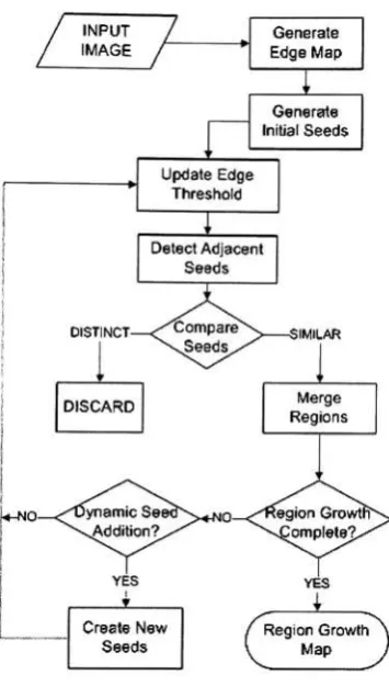
natural

images. A flowchart for

this

module

Figure

3.1:

Flowchart

of

Region

Growth Procedure

is

shown

in Fig.

3.1

andthe

detailed

explanation of each

step is described below.

3.1.1

Initial

Seed

Generation

Using

themagnitude of

the

gradient

G(i,j)

of

the

color

image

field,

computedas

de

scribed

in

2.1,

the

edge

map

of

images is

obtained.

Ideally,

a

threshold

value could

be

se

lected

to

provide us with

the

most

edges,

while

ignoring

noisepresent

in images. The

prob

lem is

that the

natureof

images

does

not allow

for

this

disposition. A

threshold that

may

correcdy

delineate

the

boundary

ofa given region

may

allow otherregions

to

be

merged.

Due

to this

factor,

we

initiate

our algorithm

by

selecting

regions

that

do

not present

any

edges

within, and,

if

such regions are not

found,

the

edge value or

threshold

is increased

until regions are

detected.

To

prevent multiple seed generation within

homogeneous

and [image:24.509.170.348.72.385.2]

connected

regions, the

region selectionat

this

stage

is

restricted

to

clusters of pixels which

are

larger

than

0.5%

of

the

image. Each individual

cluster

is

assignedaparticular

label

for

differentiating

purposes.

This label map is

referredas

the

Parent

Seeds (PS). The

labeling

procedureuses

the

_{general procedure outlined}

in

_reference

[21].

1. Run-length

encodethe

input image.

2. Scan

the runs,

assigning preliminary labels

and

recording label

equivalences

in

a

local

equivalence

table.

3. Resolve

the

equivalenceclasses.

4. Relabel

the

runs

based

on

the

resolvedequivalenceclasses.

3.1.2

Region Growth

The

procedurecontinues

by increasing

the threshold

found

in

the

initial

seed generation

and

detecting

new regions or child seeds

that

fall below

the

new

threshold.

These

child

seeds need

to

be

classified

into

adjacent-to-existent or non-adjacent seeds.

In

order

to

make

the

region growth process

efficient,

it is important

to

also

know

the

parent seed

to

which

the

child

is

adjacent.

The

objective

is

to

be

able

to

process all adjacent childseeds

in

a vectorized approach.

To

achieve

this task

weproceed

to

first detect

the

outside edges

ofthe

PS map

using

a nonlinear spatial

filter.

The

filter

operates on thepixels ofa

3

x

3

neighborhood,

and

the

response of

its

operation

is

assigned at

the

center pixel ofthe

neighborhood.

The

size of neighborhoods

being

operated will

be

assumed

to

be 3

x

3

unless specifiedotherwise.

The filter

operates

according

to

F(i,j)

= <

0

ifPS(i,j)>0,

0

if(min)e/3PS(7n,n)is0,

(3.1)

1

otherwise

where

/3

is

the

neighborhood

being

operated.

The

resultof

applying

this

filter is

a mask

indicating

the

borders

of

the

PS

map.

The

child seeds are

individually

labeled,

and

the

ones adjacent

to the

parent seeds are

identified

by

performing

an element-by-element multiplication of

the

parent seeds edge

mask and the

labeled

child map.

The remaining

pixels are referred

to

as

the

adjacent

child pixels.

The

pixels whose

labels

are members of

the

set of

labels remaining

after

the

multiplication

become

part of

the

adjacent child seeds map.

For

the

proper addition of

adjacent child

seeds,

it is necessary

to

compare

their

individual

color

differences

to their

parents

to

assure a

homogeneous

segmentation.

Reduction

of

the

number of seeds

to

be

evaluated

is

accomplished

by

attaching

to their

parents

the

child seeds

that

have

a size

smaller

to

the minimum seed size

(MSS).

In

our

algorithm, the

MSS is

set

to

0.01%

of

the

image.

The

child seed sizes are computed

utilizing

sparse matrix storage

techniques to

allow

for

the creation of

large

matrices with

low

memory

costs.

Sparse

matrices store

only

the

nonzeroelements ofthe

matrix, together

withtheir

location in

the

sparse matrix

(indices).

The

sizeof each child seed

is

computed

by

creating

a matrix of

M

x

N

columns

by

C

rows,

where

M is

the

number of columns of pixels

in

the

image,

N

the

numberof

rows,

and

C

thenumber of adjacent child seeds.

The

matrix

is

created

by

allocating

a

1

at each column

in

therow

that

matches

the

pixel

label. The

pixels

that

do

not

have

a

label

are

ignored.

By

summing

all

the

elements

along

each

row,

we obtain

the

number of pixels per child seed.

This

procedure

is

useful

for

any

operation

that

requires

the

knowledge

of

the

number of

elements per

group in

the

segmentation algorithm.

To

attach regions anassociation

between

childseeds and

their

parents

is

required.

The

adjacent child pixelsprovide

the

child

labels,

but

not

the

parent

labels. A

new spatial

filter

is

applied

to the

PS map

to

obtain

the

parent

labels.

The

filter

response at each center

point

is

equal

to

themaximumpixel value

in

its

neighborhood.

The

association

between

child and parent can now

be

obtained

by

creating

a matrix with

the

first

column composed

of

the

adjacentchild pixels and

the

second

column,

with

labels found

at

the

location

of

the

adjacent child pixels

in

the

matrix obtainedafter

applying

the

maximum value

filter

to the

PS

map.

It is important

to

note

that

non-linear

filters

are used

to

provide

information

about

the

seeds and not

to

directly

manipulate

the

image;

therefore,

it

does

not

impair

the

final

result.

The

functionality

of the association matrix

is

manifold.

It

provides

the

numberof child

pixels

that

are attached

to

parent seeds andalso

identifies

which child seeds share edges

with more

than

one parentseed.

Child

seeds smaller

than

MSS

can now

be

directly

at

tached

to their

parents.

Child

seeds

that

share

less

than

5

pixels with

their

parents and are

larger

than

MSS

arereturned

to the

unsegmented region

to

be

processed when

the

region

shares a moresignificant

border.

Finally,

the

remaining

seeds are compared

to their

parents

to

analyze

if

they

should

be

added

to

a parent seed or not.

Given

thatspatial regions

in

images

vary

gradually,

only

the

nearby

area of

adjacency

between

parent and child

is

compared

to

provide a

true

representation of

the

color

differ

ence.

This

objective

is

achieved

by

using

two

masks

that

will exclude

the

areas of

both

parent and child seeds

that

are

distant from

their

common

boundaries.

The

first

mask

is

a

dilation

of

the

PS map using

an octagonal

structuring

element with a

distance

of

15

pixels

between

thecenter pixel

to the

sides ofthe

octagon,

as measured

along

the

horizontal

and

vertical axis.

The

second mask

is

the

same

dilation but

this time

applied

to the

adjacent

child seeds map.

The

two

masks

mutually

exclude

the

pixels

that

fall beyond

eachother's

dilation

masks.

The

values used

in

our algorithm are optimized

to

work with

images

that

range

from 300

x

300

pixelsof resolution

to

1000

x

1000

pixels.

The

comparisonof regions

is

performed

using

the

Euclidian

distance between

themean

colors of

the

groups.

The

reason

for

choosing

this

method

is

that

only

the

nearby

areaof re

gions

is

being

compared, and,

therefore,

the

increased complexity

of

using

the

Mahalanobis

distance does

not

improve

the results,

because

the

variance of

the

regions compared will

be

small.

Also,

prior

to

comparing

the colors, the

image is

converted

to the

CEE

L*a*b*

color

space,

assuring

that

comparing

colors

using

the

Euclidean

distance is

similar

to the

differentiation

of colors

by

the

human

eye.

The

maximum color

distance

to

allow

the

in

tegration

of

the

child seed

to the

parentseed

is

set

to

20. This distance is

chosen

to

allow

the

differentiation

ofat

least 10 different

colors

along

the

range of

the

a*

channel or b* channel.

3.1.3

Dynamic Seed Generation

When

the

parent seeds are created

in

the

initial

seed

generation,

theregions represented

by

these

seeds are characterized

by

areas of

the

image

that

have

no

texture.

These

areas

can

be instances

of

sky, water, skin,

and

in

general,

regions where

there

is

either no color

variance or a gradual

transition

from

one color

to the

next.

The

dynamic

addition of seeds

to the

PS

map

is

ouranswer

to

include

the

remaining

regions

that

display

different

levels

of edge

intensities

through them

but

are part of

the

same

identifiable

object.

Dynamic

seed

generation consist of

selecting

a set of

threshold

values at which additional seeds are added

to the

parent seeds.

The

threshold

values are adjusted

to

account

for

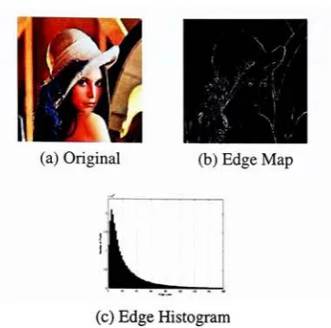
the

exponential

decay

of edge values as seen

in Fig.

3.2.

Ranges in

the

low-edge

values account

for large

areas

in

the

image.

To incorporate

new

areas, the threshold

values need

to

increment

exponen

tially

to

include

additional elements of considerable size

into

the

segmentation map.

The

threshold

values selected

for

the

addition of new seeds are:

15, 20, 30, 50, 85,

and

120

accounting

for

an

increment

of

10%

of

the

area of

the

image

added at each

interval.

At

these

intervals,

theadditionof new seeds

follow

a similar procedure

to the

method

explained

in

3.1.2.

The

regions

that

fall

below

the

selected edge

threshold

are

detected.

All

the

regions thatare not attached

to

any

parent seeds and are

larger

than the

MSS

are

added

to the

PS

map.

For

the

additionof new seeds

that

share

borders

with existent

seeds,

they

are required

to

meet

two

qualifications:

1)

the

group

must

be large

enough

to

become

a

group

by

itself,

and

2)

thecolor

differences

between

the

regionand

its

neighbor must

be

greater

than the

maximumcolor

difference

allowed.

(a)

Original

(b)

Edge

Map

[image:29.509.177.359.71.251.2]

(c)

Edge Histogram

Figure 3.2: Histogram

of

Edge

Values for Lena

3.1.4

Seed Growth

Tracking

and

Classification

Region

growth without

feedback

of

the

growth rate of each seed

may

cause parent seeds

to

overflow

into

regions of similar colors

but different

textures.

Regions in images

display

similar edge

density

throughout

the region;

therefore,

to

maintain

homogeneity,

the

regions

thatare createdat

low

gradient

levels

and slow

their

growth rateshould

be

classified as a

grownseed and should

be

removed

from

thegrowth procedure.

The

size

tracking

of each seed

is

performedat each

dynamic

seed addition

interval. The

number of pixels per seed

is

computedateach

interval,

and when

the

increment

ofa parent seed

does

not reach above

5%

of

its

original

size, the

growthofthis seed

is

stopped.

When

the

last interval has been

reached,

all

the

identifiable

regions

have

been

given a

label

and all

remaining

areas are

edges ofthesegmented regions.

At

this

stage all seeds are allowed

to

grow

to

complete

the

region growth procedure.

3.2

Texture

Channel Generation

Much

of

the

problem

in image

segmentation algorithms

is

caused

by

the

presence of

regions

that

contain

distinct

patterns.

The

issue is

that

patterns arecomposedofmultiple

shadesofcolors and cause

over-segmentation

andmisinterpretation of

the

edges surround

ing

the

patterned object.

These

objects are referred

to

in

the

computer vision

industry

as

textures.

Texture

regions

may

contain regular patterns such as a

brick

wall, to

irregular

patterns suchas

leopard

skins,

bushes

and

many

objects

found in

nature.

The

presence of

texture

in images is

so

large

and

descriptive

ofobjects

that

we

have

decided

to

generatean

additional channel

containing

this

important information.

A

method

for obtaining information

ofpatterns within an

image is

to

evaluate

the

ran

domness

presentat various areas of

the

image.

Entropy

provides a measure of

uncertainty

of a random variable

[22].

If

the

random variable

is

composed

from

the

pixel values of

a

region, the

entropy

will

define

the

randomness associated

to the

region

being

evaluated.

Texture

regions contain various colors and

shades;

therefore,

texture

regions will containa

specific value of

uncertainty

associated with

them, providing

a structure

to

merge regions

that

display

similar characteristics.

Information

theory

introduces

entropy

as

the

quantity

which agrees with

the

intuitive

notion of what a measure of

information

should

be [22]. In

accordance with

this

supposi

tion,

wecan select a random

group

of pixels s

from

an

image,

with a set of possible values

{ai,

a2,

. . .

,aj}.

The probability

for

a specific value

a,

to

occur

is

P(dj),

and

it

contains

I

(aj)

=

l9p-(\

= _~l9p

(aj)

(3-2)

units of

information. The

quantity

/(%)

is

referred

to

as

the

self-information ofa,.

If

k

values are present on

the set, the

law

of

large

numbers stipulates

that, for

a

sufficiently

large

value of

k,

symbol

%

will on average

be

output

kP(dj)

times.

Thus

the

average

self-information obtained

from

k

outputs

is

-kP

(ai)

logP

(ai)

-...-kP

(aj)

logP

(aj)

(3.3)

or

j

-kJ2P(aj)logP(aj).

(3.4)

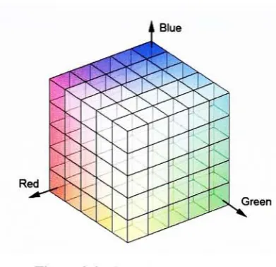
Red

[image:31.509.153.349.64.253.2]

Green

Figure 3.3: Quantization

of

Colors

The

average

information

persource

output,

or

entropy is defined

by

H(s)

=

~'P(aj)logP(aj)

(3.5)

This quantity is defined for

a single random

variable,

and

for

the

case of

color,

multiple

variablesare used.

To

take

advantageofthecolor

information

without

extending

the

pro

cess

to

compute the

joint

entropy,

the colors

in

an

image

are quantized

into

63,

or

216

different

colors.

The

quantization of colors can

be done using

uniform quantization which

cuts

the

RGB

color cube

into

smaller

boxes,

and

then

maps all colors

that

fall

within each

box

to

thecolorat

the

center ofthat

box.

Uniform

quantization

is

represented

in

Fig.

3.3.

After

the

colors

have been

quantized,

eachpixel of

the

image

can

be indexed

to

one of

the

216

representative

colors,

effectively reducing

the

probability

of each color

occurring

to

a one-dimensional random variable.

To

create

the texture channel, the

local entropy

is

computed on a

9-by-9

neighborhood around each pixel

in

the

indexed

image,

and

the

resulting

value

is

assigned

to the

center pixel of

the

neighborhood.

3.3

Multiresolution

Region

Merging

The

texture

channel obtained

from

the

second module

is

combined with

the

color

infor

mation

to

describe

the characteristicsof each region segmented

by

theregion growth mod

ule.

Using

amultivariate analysis of

the

independent

regions, the

resultant

Mahalanobis

distances between

groups

is

used

to

merge similarregions.

To

this

point

the

segmentationof

the

image has been

performed with an absence of

information

about

the

individual

regions.

Now

that the

image has been

segmented

into

different

groups,

information

can

be

gathered

from

each

individual

region.

Given

that

we

have four

sources of

information

(Red, Green, Blue,

and

Texture)

and

individual

regions

displaying

a

different

number of pixels per

group,

we require a suitable method

to

display

the

data in

order

to

investigate

relationshipsof

the

regions.

The data

can

be

modeled

using

an

(N

*

P)

matrix,

where

N

is

the total

number of pixels

in

the

image,

and

P

are

the

total

number of variables

that

contain

information

about each pixel.

G is

the total

number

of groups

in

which

the

image has been

segmented

in

the

region growth

procedure; then

the matrix

is

composed of

G

separate sets.

The

objective

is

to

obtain a mean value

for

each

group

that

is

used

to

compare

the

different

groups.

The

method used

to

achieve

this

objective

is

a

one-way

analysis of

variance,

which

is

explained

in detail in

section

2.2.

The Mahalanobis-squared distances

are obtained

for

each pair of groups

from

the

one

way

analysis of

the

data. The

algorithm uses

these

distances

to

find

the

similar groups and

merge them.

Once

a

group has

been

merged, the

similarity

of

this

group

to the

others

is

unknown,

but

required

if

the

new

group

needs

to

be

merged

to

other similar groups.

To

prevent

the

need

to

re-evaluate

the

Mahalanobis distances

for

the

groups after each region

merging has

occurred,

an alternate approach was

introduced.

Having

the

distances

between

groups,

thesmallest

distance

value

is

found. This

value

only

provides one pair of

groups;

therefore,

the

similarity

value

is increased

until a

larger

set of

group

pairs

is

obtained.

Five group

pairs were

found

to

be

an adequate number of

groups

to

reducecomputation

time

without

merging

groups

inadequately. We

initiate

by

merging

the smaller

group in

this set and

then

continue

to

merge

the

next

larger

group.

After

the

first

merge,

acheck

is

performed

to

see

if

one of

the

groups

being

merged

is

now

part ofa

larger

group.

In

this

caseall

the

pair combinations of

the

groups should

belong

to

the pairs selected

initially

in

the

set

to

be

merged

together.

Once

all

the

pairs of

the

set

have been

processed, the

Mahalanobis distance

is

recom

puted

for

the

new segmentation

map,

and

the

process

is

repeated until a

desired

number of

groups

is

achieved.

The

value of

similarity

obtained,

after

the

desired

numberofgroups

has been

achieved,

should

be

used as a minimum value of

merging

to

assure

that

all

the

images

display

a similar

level

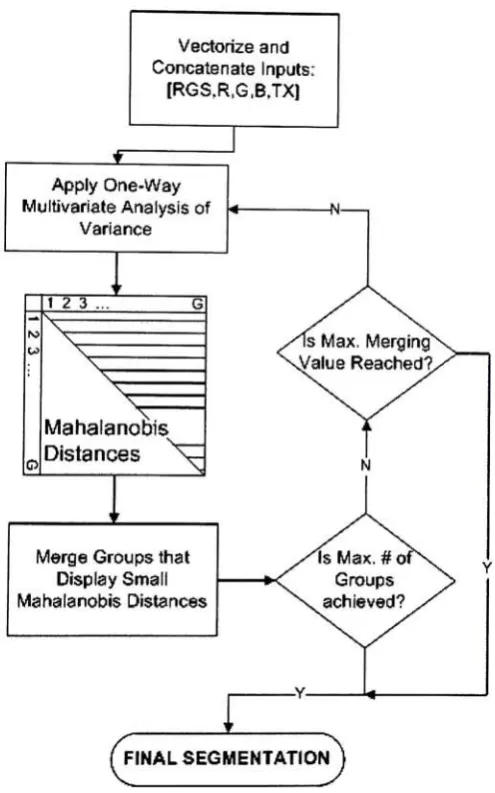
of segmentation.

A flowchart

of

the

procedure

is

shown

in

Fig.

3.4.

Vectorize

and

Concatenate

Inputs:

[RGS,R,G,B,TX)

Apply One-Way

Multivariate Analysis

of

Variance

o

1 2 3 ...

v;

X

x~

x:

Mahala

nobis

Distances

\^

Merge Groups

that

Display

Small

Mahalanobis

Distances

Figure

3.4:

Flowchart

of

Merging

Procedure

[image:34.509.131.379.151.548.2]

Chapter

4

Results

Until

recently,

different

_{segmentation algorithms proved}

their

effectiveness

by display

ing

the

results obtained on a

limited

set of

images. Hebert

et al

introduced

a method

for

actually assigning

aquantitativevalue

to the

quality

of a givensegmentation

by

calculating

the

Normalized Probabilistic Rand

(NPR)

index [19].

The

technique

involved

in

the

calcu

lation

of

the

NPR index is

summarized

in

section

2.3. Because

the

NPR

providesa value

which

is

directly

related

to the

manualsegmentationsutilized

in

the

evaluation

process,

a

set of manualsegmentations

is

required

that

display

the

following

characteristics:

1. It

cannot

be

chosen

selectively

to

favor

a givenalgorithm.

2.

It

displays

variousscenarioswithmultiple

levels

of complexity.

3. It

containmore

than

one

individual

perspective.

4. It

can

be

accessed

by

anyone

to

perform

the

same

test

on

diverse

algorithms.

Table

4.1: Segmentation

algorithm results

GRF

JSEG

GSEG

Avg. Time

(sec)

280

28

46

Avg.

NPR

0.358

0.440

0.486

Std. Dev. NPR

0.345

0.319

0.313

Environment

C

C

MATLAB

[image:35.509.139.367.537.644.2]

GRF NPRdistribution _{JSEG NPR distribution GSEG NPR distribution}

lj a

-06 -04 -0.3 D 0.3 04 06 08 I

a

$.6 -OB -04 -0.2 0 02 04 0.6 08 NPR index [image:36.509.47.467.79.218.2]

(a)

(b)

(c)

Figure 4.1: Distribution NPR

scores.

(a)GRF; (b)JSEG;

(c)GSEG

Such

a set

is

available on

the

publicly

accessible

Berkeley

Segmentation

Database. This

database

provides

1633

manual segmentations

for 300 images

created

by

30 human

sub

jects [23]. State-of-the-art

algorithms werechosen

to

compare

the

quality

of

the

segmen

tation

results.

These

segmentation

techniques

are

Fusion

of

Color

and

Edge

Information

for improved Segmentation

and

Edge

Linking

(GRF)

[6],

the

unsupervised segmentation

of color-texture regions

in images

andvideo

(JSEG)

[16],

and

the

novel algorithmauto matic segmentation

by

dynamic

region growth and multiresolution

merging (GSEG). To

prevent

any

discrepancy

at

the

time

of

comparing

the results,

all

the

available

images

were

segmented

using

the

available segmentation algorithms onthesame machine.

The

testing

computer

has

a

Pentium

4

CPU

3.20GHz,

and

1.00 GB

of

RAM. The

GRF

and

JSEG

al

gorithms wererun

from

theexecutable

file

provided

by

Rochester

Institute

of

Technology

and

the

University

of

California

respectively.

The

proposed method was processed

using

MATLAB

R2006a.

The

normalization

factor

was computed

by

evaluating

the

Probabilistic Rand

(PR)

for

all available manual

segmentations,

and

the

expected

index

obtained was

0.6064. Results

obtained

for

the

distinct

methods are

displayed

in

table

4.1.

The

results show

that the

GSEG

algorithm

has

the

highest

overall

NPR

results,

and

the

varianceof

the

results

has

the

narrowest

spread,

proving

that

the proposedalgorithm performs

consistently

better

than

the

otheralgorithms.

Fig. 4.1

display

the

distribution

of

the

NPR

scores

for

all

the tested

images.

It

can

be

observed

that

273

out of

300 images using

the

proposedalgorithm are

(a)

Original

(b)GRF

[image:37.509.109.408.76.405.2]

(c)

JSEG

(d)

GSEG

Figure 4.2:

Balloon

Results

distributed into

the

top

half

or acceptable segmentation range.

This is

similar

to the

number

of segmentations

that

fall

withinthisrange

using

the

JSEG

algorithm.

The

actual

improve

ment can

be

seen

in

the

number of segmentation scores

that

fall

within

the

range of

very

good segmentation results

[0.7

<

NPR

<

1]. These

numbers

for

the

GRF, JSEG,

and

GSEG

were

47, 74,

and

98

respectively.

This

indicates

that

close

to

a

third

ofthe

images

segmented

using

our algorithm match

closely

to the

segmentations performed

by

human

beings. The

evaluation of

the

segmentationalgorithms were performed

by

maintaining

the

standardparameters available as the

inputs

for

the

segmentationprograms.

Some

of

the

results obtained

from running

the

GSEG

algorithm,

as well as the other

segmentationsmethods without

any

parameter

tuning

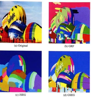
areshown

in Figs. 4.2

-

4.7. Clear

(c)

JSEG

(d)

GSEG

Figure

4.3: China

Results

(a)

Original (b)GRF

(c)

JSEG

(d)

GSEG

Figure

4.4:

Pilot Results

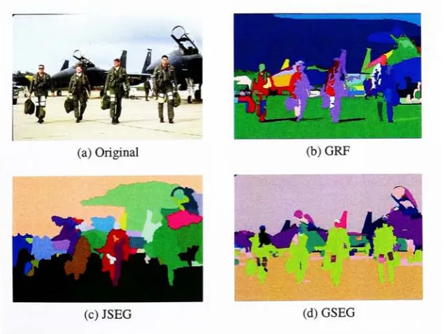
[image:38.509.95.416.91.325.2] [image:38.509.95.417.381.623.2]

(a)

Original

(b)

GRF

(c)

JSEG

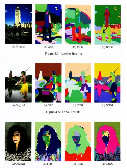
Figure

4.5:

London Results

(d)

GSEG

(a)

Original

(b)

GRF

(c)

JSEG

Figure 4.6: Tribal Results

(d)

GSEG

(c)

JSEG

Figure 4.7:

Lady

Results

[image:39.509.43.472.68.633.2]

advantages can

be

seen on

the

level

of

detail

achieved

from

our segmentation

in

comparison

to the

JSEG

segmentation

for

all

the

images. The boundaries

of

the

GRF

procedurematch

directly

the

boundaries

ofthe object

in

the

image.

Fig.

4.4(c),

and

Fig.

4.5(c)

displays

the

disadvantage

of

guiding

the

segmentationmethod

based

on

the

quantizationof colors

to

create

the

initial

clusters.

In

these

images

the

sky has

been

oversegmented,

because

the

change of

light

provides

different

shades of

blue. Advantages

of

the

multiresolution

merging

method can

be

seen on

Figs.

4.3(d)

and

4.7(d).

In

these

results multiple regions

that

create a pattern are assigned

to the

same

class,

allowing

the

algorithm

to

reducethe total

number of classes without

losing

information

obtained

from

multiple similar regions

that

are not adjacent

to

each other.

The

GRF

results

have

the

same

level

of

detail

as

the

GSEG

approach,

but its lack

of

texture

modeling

does

not allow

it

to

differentiate

objects with

similar colors

but

different

texture.

Figs.

4.4(b), 4.5(b),

and

4.6(b)

have

regions merged

that

display

similarcolors

but

contain

substantially different

textures.

Chapter

5

Conclusion

This

work provides aneffective method

for

automatic

image

segmentation on simple

to

complex

images.

The

algorithm

is based

on color edge-detection and

dynamic

region

growing,

completed

by

a multiresolution region merging.

The

segmentation procedure

has

been

tested

on

the

publicly

available

Berkeley

database,

and

the

quality

of

its

results

has

been

measured.

The

robustness of our algorithm

is displayed

on

the results,

along

with

those

obtained on

the

same

image

when segmented

by

other methods.

Future

research

would

be focused

on object classification

based

on

this

segmentation algorithm.

References

[1]

J. B.

McQueen,

"Some

methods

for

classificationand analysis ofmultivariate obser vat