Remaining Useful Life Assessment of Lithium-ion Battery based on HKA-ELM Algorithm

Int. J. Electrochem. Sci., 13 (2018) 9257 – 9272, doi: 10.20964/2018.10.51

International Journal of

ELECTROCHEMICAL

SCIENCE

Remaining Useful Life Assessment of Lithium-ion Battery based

on HKA-ELM Algorithm

Jing Yang1,2,3_{, Zhen Peng}4_{, Zhaodi Pei}1,2,3_{, YongGuan}1,2,3_{, Huimei Yuan}1,2,3_{, Lifeng Wu}1,2,3*

1 _{College of Information Engineering, Capital Normal University, Beijing 100048, China}

2 _{Beijing Key Laboratory of Electronic System Reliability Technology, Capital Normal University,}

Beijing 100048, China

3 _{Beijing Advanced Innovation Center for Imaging Technology, Capital Normal University, Beijing}

100048, China

4 _{Information Management Department, Beijing Institute of Petrochemical Technology, Beijing 10217,}

China

*_{E-mail: wulifeng@cnu.edu.cn}

Received: 5 May 2018/ Accepted: 30 July 2018 / Published: 1 September 2018

Accurately predicting the remaining useful life (RUL) of lithium-ion batteries is very important to battery management systems (BMS). Recently, Extreme Learning Machine (ELM) algorithm has been applied to RUL prediction of lithium-ion batteries. However, the input weights and biases of the ELM algorithm are generated randomly, which affect its prediction accuracy. In this paper, we use the heuristic Kalman algorithm (HKA) to optimize the input weights and biases of the ELM algorithm. The mean square error (MSE) obtained from the ELM is used as the cost function of the HKA algorithm, and the optimized particles in the HKA are used as the weights and biases of the ELM predictor. In this work, the HKA-ELM method is introduced firstly, then, we perform experiments on the battery data set to verify the proposed algorithm, and compare with other algorithms. Results show that our proposed method has better prediction accuracy than related works.

Keywords: Lithium-ion battery, RUL prediction, ELM, HKA

1. INTRODUCTION

important [2,3]. The RUL is defined as the number of charge and discharge cycles before the battery performance drops to the rated failure threshold [4].

The existing literature methods for lithium-ion battery RUL prediction can be divided into two types, the model-based method and the data-driven method [5]. The model-based method requires an understanding of the compositions of the model, and it describes the degradation model from the internal working mechanism by using the mathematical model [6]. The literature [7] uses a hybrid

method to predict the RUL of lithium-ion battery, including unscented Kalman filter, complete ensemble empirical mode decomposition and relevance vector machine. In [8], the particle filter is proposed to predict the RUL. In [9], the particle filter (PF) algorithm is improved by HKA, and the improved PF algorithm predicts RUL of lithium-ion battery. Chen and Miao [10] employ the artificial fish swarm algorithm method with variable population size (AFSAVP) as an optimizer for the parameters of adaptive bathtub-shaped function (ABF), and then use the optimized algorithm to predict the RUL of lithium-ion battery. The literature [11] proposes the unscented particle filter (UPF) for the battery RUL prediction, and in [12], the authors propose the improved unscented particle filter (IUPF) algorithm to estimate the RUL. However, due to the complex internal characteristics of lithium-ion batteries, it is difficult to implement the model-based method [13].

The data-driven method has been applied to the RUL prediction of lithium-ion battery and achieved significant results [14]. It monitors the state of the system, analyzes its state behavior from historical data, and transforms it into related models, to predict the future state [15]. The main idea is to regard lithium-ion batteries as black boxes without considering the complex electrochemical processes and structures in the model, meanwhile analyze its state behaviors from historical data, and transform it into related models. According to the training samples, the implicit information between the input and the output is obtained, and finally the future trend is predicted. Therefore, the algorithms or related parameters are the main factors affecting the accuracy of RUL prediction [16]. Zhao [17] combines feature vector selection (FVS) with support vector regression (SVR) to estimate the RUL of lithium-ion battery. The literature [18] estimates the lithium-ion RUL by combining the Dempster– Shafer theory (DST) and the Bayesian Monte Carlo (BMC) method. In [19], on-line lithium-ion battery prediction is realized by the incremental optimized relevance vector machine (IP-RVM) algorithm, which improves the accuracy. In addition, artificial neural network (ANN) has been applied to the prediction of the RUL of lithium-ion batteries with better flexibility and easier implementation [20]. In [21], an ANN method is proposed and has achieved pretty results.

the problems of welded beam design and the robust PID design [26]. In this paper, HKA is used for optimizing ELM algorithm for better accuracy.

The rest of the paper is organized as follows: in the second part, the theory of the proposed method is briefly introduced, including the basic principles of ELM algorithm, HKA algorithm and the HKA-ELM algorithm. The third part presents a description of our experiment method. The experimental results and the discussion are in the fourth part. We summarize this paper in the final section.

2. RELATED ALGORITHMS

This part describes the basic principles of ELM algorithm, HKA algorithm and HKA-ELM algorithm.

2.1. Extreme learning machine

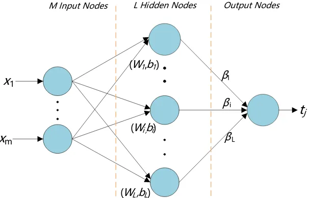
The ELM algorithm is a feed forward neural network with a single hidden-layer proposed by Huang. It has the ability of fast learning. The network consists of three layers: the input layer, the hidden layer and the output layer [22]. In this neural network, the weights and biases are generated randomly, then the output weights are determined according to the least-squares method [27]. Its structure is shown in Fig. 1.

β1

β i

β L

(W1 ,b1 )

(Wi ,bi )

x1

xm

(WL ,bL )

tj

M Input Nodes L Hidden Nodes Output Nodes

Figure 1. ELM network structure

The matrix [x1, x2, ..., xm] is the input matrix, and m is the number of inputs. tj is the output, j=1,

2, ..., m.

The input matrix W is represented by: 𝑊 = [

𝑤₁₁ ⋯ 𝑤_1𝑚

⋮ ⋱ ⋮

In Eq. (1), l is the number of hidden nodes. The bias matrix b is represented as: 𝑏 = [

𝑏1

⋮ 𝑏_𝑙

]

𝑙×1

(2) Assuming that the activation function is G(x), the output matrix H of the hidden layer can be represented as:

𝐻 = [

𝐺(𝑤₁, 𝑏₁, 𝑋₁) ⋯ 𝐺(𝑤_𝑙, 𝑏_𝑙, 𝑋_𝑙)

⋮ ⋱ ⋮

𝐺(𝑤₁, 𝑏₁, 𝑋_𝑛) ⋯ 𝐺(𝜔_𝑙, 𝑏_𝑙, 𝑋_𝑛) ]

𝑛×𝑙

(3) The output tj in Fig.1 is expressed as:

∑ 𝛽_𝑖

𝑙

𝑖=1

𝐺(𝜔_𝑖, 𝑏_𝑖, 𝑥_𝑗) = 𝑡_𝑗, 𝑗 = 1,2, … , 𝑚 (4) that is:

𝐻𝛽 = 𝑇 (5)

The ELM algorithm steps [28] are as follows:

Step1. Determine the number of hidden layer nodes l, and randomly generate the input weight W and the hidden layer bias b;

Step2. Determine the activation function G(x) and calculate the output matrix H of the hidden layer;

Step3. Calculate the output weights. According to Eq. (5), the output weight β is determined by the generalized inverse operation of the hidden layer matrix. The expression is:

𝛽 = 𝐻+_{𝑇, (6)}

where H+ is the Moore–Penrose generalized inverse of H [28]. 2.2. Heuristic Kalman algorithm

HKA is an optimization algorithm, which takes the optimization problem as a measurement process to get the best estimate. It is an iterative process [25]. The HKA algorithm schematic is shown in Fig.2.

p

(x)

(random genetate

m

S

)

cost function

J(.)

N

x

(i)(i=1,2,..N)

J(x

)

Measurement process

Kalman estimation

ξ

N

Figure 2. Principle of HKA

In the kth iteration of HKA, the vector x(k) is generated from the probability density function (pdf) pk(x), then x(k) is used as the input at the measurement process to generate the optimal value. In

the Kalman estimation process, the optimal values are combined with pk(x) to generate a new pdf

pk+1(x), which is used for reference in the next iteration [30]. The steps of the HKA [25] are as follows.

Step1. Initialization. Selecting N, Nξ and slowdown coefficient α, where N is the number of

particles and Nξ is the number of best candidates;

Setp2. Random Generator (mk, Sk). Generating a sequence of N vectors according to a Gaussian

distribution parameterized by mk and Sk;

Step3. Measurement. In the kth iteration, choosing {x1 k ,…, xk

Nξ

} as the best candidate and calculating the value of ξk and Vk

𝜉_𝑘= 1

𝑁_𝜉∑ 𝑥𝑘

𝑖 𝑁_𝜉

𝑖=1

(7)

𝑉_𝑘= 1

𝑁_𝜉[∑(𝑥1,𝑘

𝑖 _{− 𝜉}

1,𝑘)2, … , ∑(𝑥𝑛,𝑘𝑖 − 𝜉𝑛,𝑘)2 𝑁_𝜉

𝑖=1 𝑁_𝜉

𝑖=1

]

𝑇

(8) We can consider that the measurement gives a perturbed knowledge about the optimn, i.e.

𝜉_𝑘 = 𝑥_𝑜𝑝𝑡 + 𝑣_𝑘, (9)

where 𝑣𝑘 is the unknown perturbation, which is estimated by available knowledge. 𝜉𝑘 is the optimum

average value of the best candidates. 𝑉_𝑘 is the ignorance of the 𝑥_𝑜𝑝𝑡.

Step4. Optimal estimation. In the Kalman framework, the estimator is expressed in the following form:

𝑥̂_𝑘+ = 𝛬_𝑘𝑥̂_𝑘−+ 𝐿_𝑘𝜉_𝑘, (10)

where 𝑥̂_𝑘+is a posteriori estimate, 𝑥̂_𝑘− is the optimal value of a priori estimate. 𝛬_𝑘and 𝐿_𝑘are positional matrices whose purpose is to ensure that the process has minimum error estimates. The expression of the minimum error estimate is:

(𝛬_𝑘, 𝐿_𝑘) = 𝑎𝑟𝑔𝑚𝑖𝑛 𝐸[𝑒̂_𝑘+𝑇𝑒̂_𝑘+], 𝐸[𝑒̂𝑘+] = 0

(11) E is the expectation operator. The posterior estimation error 𝑒̂𝑘+ and the covariance matrix

𝑃_𝑘+ is defined as:

𝑒̂𝑘+ = 𝑥𝑜𝑝𝑡− 𝑥̂𝑘+,

𝑃𝑘+ = 𝐸[𝑒̂𝑘+𝑒̂𝑘+𝑇]

(12) In the same way, the prior estimation error 𝑒̂𝑘−and the covariance matrix 𝑃𝑘− can be defined

as:

𝑒̂_𝑘− = 𝑥_𝑜𝑝𝑡− 𝑥̂_𝑘−, 𝑃𝑘− = 𝐸[𝑒̂𝑘−𝑒̂𝑘−𝑇]

(13) Under the condition that 𝐸[𝑒̂_𝑘−] = 0, it implies that the condition 𝐸[𝑒̂_𝑘+] = 0 requires:

(𝐼 − 𝛬𝑘) = 𝐿𝑘, (14)

where I is the identity matrix. Bring Eq. (14) to Eq. (10), gives: 𝑥_𝑘

Determine 𝐿_𝑘 so that the posterior error variance is minimized. 𝐿𝑘= 𝑃𝑘−(𝑃𝑘−+ 𝑑𝑖𝑎𝑔(𝑉𝑘))−1,

𝑃_𝐾+ = (𝐼 − 𝐿_𝑘)𝑃_𝑘− (16)

For the next iteration, the mean and standard deviation are initialized as mk =𝑥̂_𝑘+, 𝑆_𝑘 =

(𝑣𝑒𝑐𝑑_(𝑃

𝑘+))−1/2. 𝑣𝑒𝑐𝑑(𝑃𝑘+) is the diagonal matrix of 𝑃𝑘+.

The expression may generally lead to a premature convergence. By introducing a slowdown factor 𝛼 , this problem can be tackled:

𝑃_𝑘+ = (𝐼 − 𝑎_𝑘𝐿_𝑘)𝑃_𝑘−,

𝑎𝑘 =

𝛼 × 𝑚𝑖𝑛 (1, (1_𝑛∑𝑛_{𝑖=1√𝑣𝑖,𝑘})

2

)

𝑚𝑖𝑛 (1, (1_𝑛∑𝑛 _{√𝑣𝑖,𝑘}

𝑖=1 )

2

) + 𝑚𝑎𝑥

1≤𝑖≤𝑛(𝑤𝑖,𝑘)

(17)

Step5. Rewrite the vector form. All the matrices (𝑃_𝐾+, 𝑃_𝑘−and 𝐿_𝑘) are diagonal, the Eqs. (15), (16) and (17) can be rewritten as:

𝑚_𝑘+1 = 𝑚_𝑘+ 𝐿_𝑘⊛ (𝜉_𝑘− 𝑚_𝑘), 𝑆_𝑘+1= 𝑆_𝑘+ 𝑎_𝑘(𝑊𝑘− 𝑆𝑘),

𝐿𝑘 = 𝑆𝑘2⁄/(𝑆𝑘2+ 𝑉𝑘),

𝑊_𝑘 = (𝑆_𝑘2 − 𝐿_𝑘⊛ 𝑆_𝑘2)1/2_,

𝑎𝑘 =

𝛼 × min (1, (_𝑛1∑𝑛_{𝑖=1√𝑣𝑖,𝑘})

2

)

min (1, (_𝑛1∑𝑛 _{√𝑣𝑖,𝑘}

𝑖=1 )

2

) + max

1≤𝑖≤𝑛(𝑤𝑖,𝑘)

,

(18)

where the symbol ⊛ represents a component wise product and the symbol ∕∕ stands for a component wise division, diag(𝑉_𝑘) and 𝑤_𝑖,𝑘 are the ith component.

Step6. Initialize the next step. Set 𝑚𝑘 = 𝑚𝑘+1, 𝑆𝑘 = 𝑆𝑘+1.

Step7. Terminate test. If the terminate rule is not satisfied, go to step2, otherwise stop. The stopping rule is expressed:

𝑚𝑎𝑥

2≤𝑖≤𝑁𝜉

|| 𝑥₁− 𝑥_𝑖||₂ ≤ 𝜌, ₍₁₉₎ where 𝑥𝑖 represents the best candidates.

2.3. HKA-ELM

ELM has better prediction ability after HKA optimizes its weights and biases. In order to further highlight the superiority of HKA-ELM, we test and compare the proposed algorithm with PSO-ELM and PSO-ELM algorithm, among which, PSO-PSO-ELM is an improved PSO-ELM algorithm based on PSO.

ξk and Vk

Satisfied? Train Set ELM Predictor mk HKA-ELM Predictor Predict Result Cost Function The first Nξ groups of particles

mk=mk+1, Sk=Sk+1,k=k+1 Measurement

Process

N, Nξ,α, k=0 and the

maximum number of iterations.

N groups of particles

N(mk,Sk) Initialization

mk+1and Sk+1 Gaussian Generator Kalman Estimates Test Set Data ① ② ③ ④ Start ⑤ ⑥ ⑥ ⑦ ⑧ ⑧ ⑨ ⑩ ⑫ ⑪ NO YES End ⑬ ⑬ ④ ⑭ ⑮ ⑯

Figure 3. The flow chart of HKA-ELM

Algorithm 1. HKA-ELM algorithm

Step1. Initialize the parameters of the ELM predictor;

Step2. Set the HKA parameters. Setting the values of N, Nξ and α, the number of

iterations k = 0 and the maximum number of iterations;

Step3. Generate ϰ(mk, Sk). In each iteration, a normal distribution set is generated

according to the mean mk and standard deviation Sk of the Gaussian generator;

Step4. Data processing. Divide data into training sets and test sets;

Step5. Random generator. According to the Gaussian distribution, N sets of particles are randomly generated from ϰ(mk, Sk);

Step6. The generated particles are used as a random parameter for HKA predictor, and the training set is brought into the ELM predictor for prediction; Step7. Use the MSE function of ELM predictor as the cost function;

Step9. Calculate the values of 𝜉_𝑘 and 𝑉_𝑘. Calculate the values of 𝜉_𝑘 and 𝑉_𝑘separately according to Eqs. (7) and (8);

Step10. Kalman update. Calculate the values of 𝑚𝑘+1and 𝑆𝑘+1 according to Eq. (18);

Step11. Initialize the next iteration. Set mk=mk+1, Sk=Sk+1, k=k+1;

Step12. Determine if the conditions are met. If the maximum number of iterations is reached or the Eq. (19) is satisfied, the iteration is ended, otherwise enter Step5; Step13. The new HKA-ELM algorithm is formed by using the optimal value mk as the

input weight and bias of the ELM;

Step14. Predict the test data. The test set is brought into the HKA-ELM predictor for prediction;

Step15. Get the predicted value.

3. EXPERIMENT

In this section, we first describe the data used in our experiments and its environment. Then the parameters of the HKA-ELM algorithm and the evaluation function of the prediction results are described.

3.1. Data description

Figure 4. Change in capacity of batteries A3, A5, A8 and A12

discharge experiments. The rated capacity is 0.9Ah and the discharge current is 0.45A [8]. Fig. 4 shows the variation of the capacity of the four data sets as the number of charging and discharging times increases. In this paper, the failure threshold is set to 80% of rated capacity, which is 0.72Ah.

3.2. Algorithm parameters and evaluation functions

In the HKA-ELM algorithm, several parameter values need to be set. Table1 shows the values of parameters in the experiment.

Table 1. HKA-ELM parameter values

A3 A5 A8 A12

N 25 25 25 25

Nξ 5 5 5 5

α 0.5 0.5 0.5 0.5

L 10 10 10 10

Training set 41 110 80 154

Test set 41 110 80 154

In Table1, N, Nξ and α are the parameters of HKA, L, training set and test set are the parameters

of ELM. Since the sample number of four data sets are different, selection of some parameters is also not the same.

This paper selects two evaluation functions to evaluate the predicted results.

a. Mean Square Error. The value reflects the relationship between the true value and the predicted value [31]. MSE is the average squared difference between the estimated values. The smaller it is, the better the performance is. On the contrary, the prediction effect is not satisfactory. Its expression is:

𝑀𝑆𝐸 = 1

𝑀∑(𝑄𝑖− 𝑄̂𝑖)

2 𝑀

𝑖=1

, (19)

where M is the number of prediction points, 𝑄𝑖 is the ith predicted value, and 𝑄̂𝑖 is ith true value.

b. Absolute Error (AE) [32]. It is the absolute error between the predicted value and the true value, and its expression is:

𝐴𝐸 = |𝑅 − 𝑅̂| (21)

where R represents the true value of RUL, and 𝑅̂ is the predicted value of RUL.

In this part, experiments are performed on the same data set using the ELM predictor and the PSO-ELM predictor. The results are compared with the ELM algorithm. In addition, the HKA-ELM algorithm is compared with some algorithms proposed in other papers.

4.1. Results

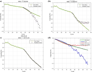
ELM algorithm and PSO-ELM algorithm are selected for comparison in this paper. The ELM parameters of the four experiment groups are the same. Fig. 5, Fig. 6, Fig. 7 and Fig. 8 correspond to batteries A3, A5, A8 and A12, respectively.

Fig.5 (a), Fig.5 (b) and Fig.5 (c) represent the prediction results of RUL using ELM, PSO-ELM, and HKA-PSO-ELM, respectively. Fig.5 (d) is the comparison of all methods and real values used in this paper. As can be seen from Fig. 5, as the method improves, the line represented by its predicted value is closer to the line represented by the true value. This indicates that the prediction effect has been significantly improved, but the prediction result of HKA-ELM algorithm represented by Fig.5 (c) is more accurate.

(a) (b)

(c) (d)

Fig. 6 is an experiment on the battery A5. The prediction results of battery A5 are obtained by applying ELM algorithm, PSO-ELM algorithm and the HKA-ELM algorithm. It can be seen that the predicted value in Fig.6 (c) is closer to its real line. Fig.6 (d) shows that the HKA-ELM algorithm has a more accurate prediction effect on battery A5.

(a) (b)

(a)

(c) (d)

Figure 6. RUL prediction results for A5

(a) _(b)

(c) (d)

Figure 7. RUL prediction results for A8

(a) (b)

(c) (d)

4.2. Discussion

Fig. 5-8 shows the prediction results of the four experimental data sets. It can be seen that the HKA-ELM algorithm has higher predictability for different data sets. Chapter 3.2 introduced two evaluation indictors. In Table 2, we listed the evaluation results of the three methods on the four data sets.

Table 2.Three algorithm evaluation results for different data sets

Battery Algorithm 𝑹̂(cycle) MSE AE A3

ELM PSO-ELM

48 0.048377

0.0066107

1 1 48

HKA-ELM 47 1.3017e-05 0

A5

ELM 161 0.036876 10

PSO-ELM 155 0.011764 4

HKA-ELM 151 2.4024e-05 1

A8

ELM 128 0.0064306 15

PSO-ELM 118 0.0028744 5

HKA-ELM 114 3.7721e-05 1

A12

ELM 174 0.20967 2

PSO-ELM 173 0.024692 1

HKA-ELM 172 1.1587e-05 0

From Table 2, we can see that for the four data sets, the MSE value of our method is only 1% of other algorithms, meanwhile it achieves the smallest AE value. The result shows the superiority of the HKA-ELM algorithm in terms of prediction accuracy.

Fig. 9 shows the variation of the MSE on different data sets using three kinds of algorithms, respectively. The variation of AE is shown in Fig. 10. In Fig. 9 and Fig. 10, each color line represents a method: the blue represents the ELM algorithm, the red represents the PSO-ELM algorithm, and the gray refers to the HKA-ELM algorithm proposed in this paper.

Figure 9. Comparison of MSE values of three algorithms in different data sets

0 0.05 0.1 0.15 0.2 0.25

A3 A5 A8 A12

The smaller the MSE value is, the stronger the prediction performance is. In Fig. 9, the gray line representing the HKA-ELM algorithm is closest to 0. Therefore, the HKA-ELM algorithm has a higher prediction performance compared with the other two algorithms.

Figure 10. Comparison of AE values of three algorithms based on different data

The AE can reflect the accuracy of RUL prediction. The closer to 0 AE is, the closer RUL prediction is to its true value. As can be seen from Fig. 10, the AE value of the HKA-ELM algorithm is closer to 0 compared with other methods, which means the algorithm is more accurate for RUL prediction.

From Fig. 5 to Fig. 10 and Table 1, we can draw a conclusion that HKA-ELM achieves better performance for the RUL prediction of lithium-ion batteries.

In this part of the paper, we further compare our methods with other literatures and the results are shown in Table 3. These literatures also use the same datasets: A3, A5, A8 and A12.

Table 3. Comparison of the HKA-ELM algorithm and other algorithms

Data Algorithm MSE AE(cycle)

A3

Hybrid [7] AFSAVP-ABF[10] UPF[11] IUPF[12] DST-BMC[18] HKA-ELM 1.9881e-04 1.789e-05 3.2627e-02 2.993e-03 7.056e-05 1.3017e-05 2 2 - 1 6 0 A5

Hybrid [7] AFSAVP-ABF[10] DST-BMC[18] HKA-ELM 1.296e-05 2.108e-02 3.025e-05 2.4024e-05 4 - - 1 A8

Hybrid [7] AFSAVP-ABF[10] DST-BMC[18] 3.364e-05 2.208e-02 1.2996e-04 4 - - 0 2 4 6 8 10 12 14 16

A3 A5 A8 A12

HKA-ELM 3.7721e-05 1

A12

Hybrid [7]

AFSAVP-ABF[10] DST-BMC[18]

HKA-ELM

4.624e-05 1.486e-02 2.401e-05 1.1587e-05

2 - - 0

In Table 3, ‘-’ indicates that there is no such value in that paper. The AE value and the MSE value of the data A3 are the smallest. Although the AE value of [12] is close to 0, its MES value is more than 10 times larger than the MSE value of the HKA-ELM algorithm. So for data A3, the proposed method has better performance.

For A5 and A8, the MSE value of method [7] is slightly larger than the value of the method proposed in this paper, but the AE values are all 4 times that of the HKA-ELM algorithm. The MSE values of methods [10] and [18] are much larger than that of this paper.

For A12, the MSE and AE values of HKA-ELM algorithm are the smallest compared with other methods.

The smaller the MSE value and the AE value, the more accurate the prediction is. Therefore, as can be seen from Table 3, HKA-ELM achieves good performance for RUL prediction of lithium-ion battery.

5. CONCLUSION

In this paper, HKA-ELM algorithm is proposed for lithium-ion battery RUL prediction. It mainly uses the HKA optimization algorithm to optimize the random parameters of ELM algorithm so as to improve its prediction ability. In the experimental part, the proposed HKA-ELM algorithm was evaluated using the lithium battery experimental data of CALCE. The experimental results are compared with the ELM, PSO-ELM algorithm and some methods proposed in other papers. The result shows that the HKA-ELM algorithm can accurately predict the RUL of lithium-ion battery.

ACKNOWLEDGEMENTS

This work received financial support from the National Natural Science Foundation of China (No.71601022), the Natural Science Foundation of Beijing (4173074), the Key Project B Class of Beijing Natural Science Fund (KZ201710028028). And the work supported by Capacity Building for Sci-Tech Innovation - Fundamental Scientific Research Funds (025185305000-187) and Youth Innovative Research Team of Capital Normal University.

References

1. J.M. Tarascon and M. Armand, Nature, 414 (2001) 359.

2. D. Wang, F.F. Yang, Y. Zhao and K.L. Tsui, Microelectronics Reliability, 78 (2017) 212. 3. L.F. Wu, X. Fu and Y. Guan, Applied Sciences, 6 (2016) 166

4. L.X. Liao, Applied Soft Computing, 44 (2016) 191.

7. Y.Chang, H.J. Fang and Y. Zhang, Applied Energy, 206 (2017) 1564.

8. Q. Miao, H.J. Cui, L. Xie and X. Zhou, Journal of Chongqing University, 36 (2013) 47. 9. P.L.T. Duong and N. Raghavan, Microelectronics Reliability, 81 (2018) 232.

10. Y. Chen, Q. Miao and B. Zhang, Energy, 6 (2013) 3082.

11. Q. Miao, L. Xie, H.J. Cui, W. Liang and M. Pecht, Microelectronics Reliability, 53 (2013) 805. 12. X. Zhang, Q. Miao and Z.W. Liu, Microelectronics Reliability, 75 (2017) 288.

13. Y.C. Song, D.T. Liu and Y.D. Hou, Chinese Journal of Aeronautics, 31 (2018) 31. 14. J. Wu, C.B. Zhang and Z.H. Chen, Applied Energy, 173 (2016) 134.

15. Y.C. Song, D.T. Liu and C. Yang, Microelectronics Reliability, 75 (2017) 142. 16. M.S. Dirk and Hülsebusch, Automobiltechnische Zeitschrift, 111 (2009) 772.

17. Q. Zhao, X.L. Qin, H.B. Zhao and W.Q. Feng, Microelectronics Reliability, 85 (2018) 99. 18. W. He, N. Williard, M. Osterman and M. Pecht, Journal of Power Sources, 196 (2011) 10314. 19. D.T. Liu, J.B. Zhou and D.W. Pan, Measurement, 63 (2015) 143.

20. J. Liu, A. Saxena, K. Goebel, B. Saha and W. Wang, Annual Conference of the Prognostics and Health Management Society, (2010).

21. X.F. Zhou, S.J. Hsieh, B. Peng and D. Hsieh, Microelectronics Reliability, 79 (2017) 48. 22. D. S. Cui, G.B. Huang and T.C. Liu, Pattern Recognition, 79 (2018) 356.

23. J. Yang, Z. Peng and H.M. Wang, International Journal of Electrochemical Science, 13 (2018) 670.

24. R. Toscano, P. Lyonnet, Information Science, 180 (2010) 1955.

25. A. Pakrashi and B.B. Chaudhuri, Information Science, 369 (2016) 704. 26. R. Toscano, P. Lyonnet, Automatica, 45 (2009) 2099.

27. Y. Lan, J.W. Hu and L.K. Niu, Measurement, 124 (2018) 378.

28. G. B. Huang, X. J. Ding and H.M. Zhou, Neurocomputing, 74 (2010) 155.

29. Y.D. Zhu, F.W. Yan, J.Q. Kang and C.Q. Du, International Journal of Electrochemical Science, 12 (2017) 6895.

30. A. Pakrashi and B.B. Chaudhuri, Information Science, 369 (2016) 704. 31. D.T. Liu, H. Wang, and Y. Peng, Energy, 6 (2013) 3654.

32. Y.P. Zhou, M.H. Huang and Y.P. Chen, Journal of Power Sources, 321 (2016) 1.