Black-Scholes for scientific computing students

Black–Scholes Option Valuation

for Scientific Computing Students

∗

Desmond J. Higham

Department of Mathematics, University of Strathclyde, Glasgow G1 1XH, Scotland

January, 2004

Abstract

Mathematical finance forms a modern, attractive source of examples and case studies for classes in scientific computation. I will show here how the Nobel Prize winning Black–Scholes option valuation theory can be used to motivate exercises in Monte Carlo simulation, matrix computation and numerical methods for partial differential equations.

1

Option Valuation for Science Students

My colleague Xuerong Mao and I designed a 24 contact hour class onThe Mathe-matics of Financial Derivatives for final year mathematics-based undergraduate students at the University of Strathclyde. The class draws together ideas from

• mathematical modelling,

• stochastics,

• mathematical analysis,

• computational methods,

and has no pre-requisites beyond freshman-level calculus and linear algebra. We have found that financial option valuation is a sexy, easily-motivated peg on which to hang a range of applied and theoretical tools. The class has proved popular,

∗_{This manuscript appears as University of Strathclyde Mathematics Research Report 01}

(2004). A revised version will appear in the Education Section of Computing in Science and Engineering, 2004.

attracting around 80% of all possible takers, including many students aiming for joint degrees in Mathematics & Computer Science, Mathematics & Physics, and Mathematics, Statistics & Economics. In this article, I focus on the computa-tional side of option valuation. Because the necessary background in finance may be introduced with little effort, realistic problems can be inserted into a range of numerical methods classes. This material is also eminently suitable as a source of open-ended, individual-study projects involving scientific computation. The article deals with three methods: Monte Carlo, binomial and finite differences. In each case, I show how the method may be used to value a European call option. Short MATLAB [5] codes are used to make the ideas concrete; these may be down-loaded fromhttp://www.maths.strath.ac.uk/~aas96106/algfiles.html. Sug-gestions for computational projects are provided.

Before discussing the three methods, I give brief reviews of the definition of a European call option and the corresponding Black–Scholes formula.

2

Financial Options

Suppose that I phone you today with the following offer:

Let’s agree now that in 3 months’ time you will have the option to purchase Microsoft Corp. shares from me at a price of $25 per share.

The key point is that you have theoption to buy the shares. Three months from now, you may check the market price and decide whether or not to exercise the option. (In practice, you would exercise the option if and only if the market price were greater than $25, in which case you could immediately re-sell for an instant profit.) This deal has no downside for you—three months from now you either make a profit or walk away unscathed. I, on the other hand, have no potential gain and an unlimited potential loss. To compensate, there will be a cost for you to enter into the option contract. You must pay me some money up front.

The option valuation problem is thus to compute a fair value for the option. More precisely, it is to compute a fair value at which the option may be bought and sold on an open market.

The option described above is a European call. The Microsoft shares are an example of an asset—a financial quantity with a definite current value but an uncertain future value. Formalizing the idea and introducing some notation, we have:

Definition A European call option gives its holder the opportunity to pur-chase from the writer an asset at an agreed expiry date t = T at an agreed exercise price E.

If we let S(t) denote the asset value at time t, then the final time payoff for the European call is max(S(T)₋E,0) because

• if S(T)_≤E the option will not be exercised.

Options were first traded in the open market in 1973. Since that time, the demand for option contracts has undergone a remarkable growth; to the extent that trading in options typically far outstrips that for the underlying assets. The popularity of options may be attributed to three facts.

1. They are attractive to speculators, who have a view on how the asset price will evolve and wish to gamble. Taking out an option generally gives a better upside (and correspondingly worse downside) than investing in the asset.

2. They are attractive to individuals and institutions wishing to mitigate their exposure to risk. Options may be regarded as insurance policies against unfavourable movements in the market.

3. There is a logical, systematic theory for working out how much an option should cost.

Points 1 and 2 create a demand for option trading and point 3 makes it viable for “marketmakers” to find sensible prices.

There is a vast array of reference material on option valuation, catering to all tastes and backgrounds. For a comprehensive treatment, ranging from the practicalities of how money is exchanged to theoretical and algorithmic aspects of option valuation, we recommend the classic finance/business-student oriented text [6]. My forthcoming undergraduate book [4] is aimed at mathematics-based students and gives equal weight to modelling, analysis and computational meth-ods. All the material in this article is covered in greater depth in [4], and pointers to some literature pertaining to the suggestions for computational projects may be found there, too. Real life option data is freely available from a number of sources, including The Wall Street Journal, The Financial Times and the Ya-hoo! Finance site http://finance.yahoo.com/. On a slightly lighter note, the fascinating story of how some of the academics behind option valuation theory tried, and eventually spectacularly failed, to put their ideas into practice with real money, is told in the highly readable book [1].

3

Asset Price Model

The Black–Scholes theory models the asset price as a stochastic process—a ran-dom variable that depends on t. From a computer simulation perspective, we need to know how to generate a typical discrete asset path. The model says that givenS0 =S(0), pricesS(ti) for the asset at timest=ti =i∆tmay be generated from the recurrence

S(ti+1) =S(ti)e(µ− 1

2σ

2

)∆t+σ√∆tξi

where

• the parameter µis the expected growth rate of the asset,

• the parameter σ is the volatility of the asset,

• ξi is a sample from a Normal(0,1) psuedo-random number generator. In MATLAB, we could compute and plot such a path as follows:

>> T = 1; N = 100; Dt = T/N; mu = 0.1; sigma = 0.3; Szero = 1;

>> Spath = Szero*cumprod(exp((mu-sigma^2)*Dt+sigma*sqrt(Dt)*randn(N,1))); >> plot(Spath)

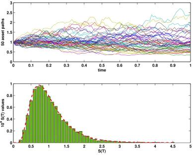
The upper picture in Figure 1 shows fifty such paths—in each case the discrete points (ti, S(ti)) are joined to give a piecewise linear curve. At the expiry date,

t=T, the asset price is a random variable with density given by

f(x) =

exp−(log(x/S0)₋(µ₋σ2/2)T)2

2σ2_T

xσ√2πT , for x >0,

with f(x) = 0 for x _≤ 0. To confirm this, the lower plot in Figure 1 gives a histogram where the final asset prices S(T) for 10,000 paths have been binned. The density curved is superimposed as a dashed line.

4

Black–Scholes Formula

In addition to employing the simple asset price model above, Black and Scholes [2] imposed a number of simplifying assumptions about the options market. Then they made creative use of the no arbitrage (“no free lunch”) principle to come up with the following formula for the value of a European call option at timet and asset price S:

C(S, t) =SN(d1)−Ee−r(T−t)N(d2),

where

d1 =

log(S/E) + (r+1

2σ

2_{)(T −t)}

σ√T ₋t , d2 = d1−σ

√

T ₋t,

and N(_·) is the Normal(0,1) distribution function,

N(x) := _√1 2π

Z x

−∞

e−s

2

2 ds.

0 0.1 0.2 0.3 0.4 0.5 0.6 0.7 0.8 0.9 1 0

0.5 1 1.5 2 2.5 3

50 asset paths

time

0 0.5 1 1.5 2 2.5 3 3.5 4 4.5 5

0 0.2 0.4 0.6 0.8 1

10

4 S(T) values

S(T)

Figure 1: Asset price paths and a histogram at expiry time.

value is C(S0,0). The MATLAB function bsf.m in Figure 4.1 gives one way of

implementing the formula, via the built-in error functionerf. An example of the function in use is

>> S = 2; t = 0; E = 1; r = 0.05; sigma = 0.25; T = 3; >> C = bsf(S,t,E,r,sigma,T)

C =

1.1447

In Figure 2 we plot a Black–Scholes surface C(S, t) as a function ofS and t. Here,T = 1 andE = 1, and we see that at expiry the option value reduces to the “hockey stick” payoff max(S₋E,0). The time zero solution C(S,0) evaluated at the initial asset price S = S0, solves the option valuation problem that we

introduced above.

European call in that the payoff depends not only on the final time asset price, but also on its behaviour over all or part of the time interval [0, T). For exam-ple, the payoff may depend on the maximum, minimum or average asset price and may knock-in or knock-out depending upon whether the asset price crosses a pre-determined barrier. Also, the option may have an early exercise facility, giving its holder the freedom to exercise before the expiry date. The design and analysis of numerical methods for valuing exotic options is still a very active re-search topic. In this article I apply the three standard approaches to the simple European call case, with the motivation that such methods are needed in more exotic circumstances.

0

0.5 1

1.5

2

2.5

0 0.2 0.4 0.6 0.8 1 0 0.2 0.4 0.6 0.8 1 1.2 1.4 1.6

S

t

Call Value

Figure 2: Black–Scholes surface for a European call.

5

Monte Carlo Method

function C = bsf(S,t,E,r,sigma,T) % function C = bsf(S,t,E,r,sigma,T) %

% Black-Scholes formula for a European call

%

tau = T-t; if tau > 0

d1 = (log(S/E) + (r + 0.5*sigma^2)*tau)/(sigma*sqrt(tau)); d2 = d1 - sigma*sqrt(tau);

N1 = 0.5*(1+erf(d1/sqrt(2))); N2 = 0.5*(1+erf(d2/sqrt(2))); C = S*N1-E*exp(-r*tau)*N2; else

C = max(S-E,0); end

Listing 4.1: Listing of bsf.m

settingµ=rin the asset model and computing the average of the payoff over all asset paths. In practice, this may be done by Monte Carlo simulation—average the payoff over a large number of asset paths. For a European call option we only need to know about the asset price at expiry, so we may take ∆t = T in each path. A suitable pseudocode algorithm is

for i = 1 to M

set Si =S0e(r−

1

2σ

2

)T+σ√T ξi set Pi =e−rTmax(Si−E,0) end

set Pmean = _M1 PM_i=1Pi

set Pvar = _M1₋₁P_iM₌₁(Pi−Pmean)2

Here, Pi is the payoff from the ith asset path, discounted by the factor e−rT to allow for the fact that the payoff happens at the future time t = T. The overall average Pmean is our Monte Carlo estimate of the option value. The

computed variance, Pvar, may be used to give an approximate 95% confidence

interval [Pmean−1.96

p

Pvar/M, Pmean+ 1.96

p

Pvar/M]. Loosely, for sufficiently

latgeM this interval will contain the true option value for 95 simulations out of every 100.

In Listing 5.1 we give a MATLAB code that applies the Monte Carlo method. Here, we have made use of the “vectorized” mode of the random number generator and the high-level commands meanand std. The output is

% MC Monte Carlo valuation for a European call %

%%%%%%%%%% Problem and method parameters %%%%%%%%%%%% S = 2; E = 1; r = 0.05; sigma = 0.25; T = 3; M = 1e6; randn(’state’,100)

%%%%%%%%%%%%%%%%%%%%%%%%%%%%%%%%%%%%%%%%%%%%%%%%%%%%%

Svals = S*exp((r-0.5*sigma^2)*T + sigma*sqrt(T)*randn(M,1)); Pvals = exp(-r*T)*max(Svals-E,0);

Pmean = mean(Pvals)

width = 1.96*std(Pvals)/sqrt(M); conf = [Pmean - width, Pmean + width]

Listing 5.1: Listing of mc.m

1.1453 conf =

1.1435 1.1471

and we recall that the Black–Scholes formula for these parameter values gave C = 1.1447. In Figure 3, we show how the Monte Carlo approximation varies with the number of samples, M. Here we took S = 10, E = 9, r = 0.06, σ = 0.1 and

T = 1. The crosses in the picture give the Monte Carlo approximations and the horizontal lines show the extent of the confidence intervals. The Black–Scholes value is represented as a vertical dashed line.

Project Suggestions

• Investigate the use of Monte Carlo for valuing a range of path-dependent options; that is, options with a payoff that depends uponS(t) for 0_≤t_≤T.

• Experiment withvariance reduction methods for speeding up Monte Carlo computations.

• Investigate the use of low discrepancy sequences and Quasi Monte Carlo methods in the context of option valuation.

• Test whether Monte Carlo may be used to compute approximations to Greeks, that is, partial derivatives of the Black–Scholes value C(S, t) with respect toS,t or parameters such asσ and E.

6

Binomial Method

1.2 1.3 1.4 1.5 1.6 1.7 1.8 1.9 2 2.1 2.2 101

102 103 104 105 106

Num. Samples

Call Value Approximation

Figure 3: Monte Carlo approximations and confidence intervals for a European call option.

ti =i∆t. Given asset price S0 at time zero, it is assumed that the asset price at

timet1 arises from either a downward movement todS0 or an upward movement

touS0, where d <1 andu >1. Then at timet2 the same restriction to down/up

movements leads to three possible asset prices d2_S

0, duS0 and u2S0. Continuing

this argument, there will bei+ 1 possible asset prices at timeti =i∆t, given by

S_ni =di−n_un_S

0, 0≤n ≤i.

At expiry time, ti = tM = T, there are M + 1 possible asset prices {SnM}Mn=0.

Letting_{CM

n }Mn=0 denote the corresponding expiry time payoffs from a European

call option, we know that

CM

n = max(SnM −E,0), 0≤n ≤M.

The binomial method proceeds by working backwards through time. An option value Ci

average of the two asset prices Ci+1

n and Cni+1+1 from time ti+1. The formula is

Cni =e−r∆t pCni+1+1+ (1−p)Cni+1

, 0_≤n_≤ i, 0_≤i_≤M ₋1.

Here, the parameterpmay be regarded as the probability of an upward movement in the asset price. The formula allows us to reverse back to time zero and compute the required option value C00. The method parameters ∆t, u, d and p must be

chosen so that the binomial asset model matches the Black–Scholes version in the ∆t _→0 limit. Once ∆tis fixed, this leads to two equations for the three remaining parameters, and consequently many possible solutions. A popular choice is

d=A₋√A2_{−1, u=A+}√_A2_{−1, p=} e

r∆t_−d

u₋d ,

whereA= 1₂e−r∆t_+e(r+σ2)∆t_.

In Listing 6.1 we list a MATLAB code that implements the binomial method, using a matrix-vector product to work backwards through time. The approximate option value W = 1.1448 agrees well with the Black–Scholes value C = 1.1447

from above.

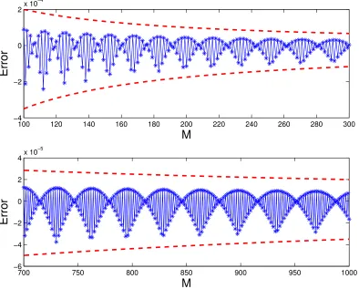
Figure 4 shows how the error in the binomial approximation behaves as a function ofM, in the caseS = 5,E = 3,T = 1,r = 0.06 andσ = 0.3. The upper picture covers 100 _≤ M _≤ 300 and the lower picture covers 700 _≤ M _≤ 1000. It is clear that although the error is generally decreasing, the convergence is by no means monotonic with M. The dashed lines in the pictures have the form “constant/M”—it may be shown that the error converges at this rate. The highly oscillatory nature of the convergence has been the subject of a number of research articles.

Project Suggestions

• Can the execution time of binom.m be improved? (See [3] for a discussion of this issue.)

• A key advantage of the binomial method is its ability to incorporate anearly exercise facility. Follow this up by implementing the method forAmerican, Bermudan orshout options.

• Investigate the literature on curbing the oscillations in the binomial error.

100 120 140 160 180 200 220 240 260 280 300 −4

−2 0

2x 10

−4

M

Error

700 750 800 850 900 950 1000

−6 −4 −2 0 2

4x 10

−5

M

Error

Figure 4: Error in binomial method as a function of M.

7

Finite Differences for the Black–Scholes PDE

The Black–Scholes formula for the value of a European call option arises as the solution of a partial differential equation (PDE). The PDE is of parabolic form, with Dirichlet boundary conditions. Unusually, a final time, rather than initial time, condition completes the problem. Letting τ = T ₋t denote the time to expiry, we may convert to a more natural initial time specification. The PDE then has the form

∂C ∂τ −

1

2σ

2_S2∂2C

∂S2 −rS

∂C

∂S +rC = 0,

with initial data

C(S,0) = max(S(0)₋E,0)

and boundary conditions

%BINOM Binomial method for a European call %

%%%%%%%%%% Problem and method parameters %%%%%%%%%%%% S = 2; E = 1; r = 0.05; sigma = 0.25; T = 3; M = 256; dt = T/M; A = 0.5*(exp(-r* dt)+exp((r+sigma^2)*dt)); d = A - sqrt(A^2-1); u = A + sqrt(A^2-1);

p = (exp(r*dt)-d)/(u-d);

%%%%%%%%%%%%%%%%%%%%%%%%%%%%%%%%%%%%%%%%%%%%%%%%%%%%%

% Option values at time T

W = max(S*d.^([M:-1:0]’).*u.^([0:M]’)-E,0);

B = (1-p)*eye(M+1,M+1) + p*diag(ones(M,1),1); B = sparse(B);

% Re-trace to get option value at time zero for i = M:-1:1

W = B(1:i,1:i+1)*W; end

W = exp(-r*T)*W;

Listing 6.1: Listing of binom.m

on the domain S_≥0 and 0_≤τ _≤T. Truncating the S range to 0_≤S _≤L and using a finite difference grid _{jh, ik_} with spacingsh=L/Nx and k =T /Nt, we may compute a discrete solutionVi

j ≈C(jh, ik). Letting

Vi :=

       Vi 1 Vi 2 ... ... Vi Nx₋1

      

∈RNx₋1

denote the numerical solution at time leveli, we have V0

specified by the initial data, and the boundary values Vi

0 and VNix for all 1 ≤ i ≤ Nt specified by the boundary conditions. Using a forward difference for thet-derivative and central differences for theS-derivatives gives the explicit method

V_ji+1₋Vi j

k −

1

2σ

2_(jh)2 Vji+1−2Vji+Vji−1

h2 −rjh

_Vi

j+1−Vji−1

2h

+rV_ji = 0.

The method may be expressed in matrix-vector form

Vi+1 =FVi+pi, for 0_≤i_≤Nt−1, whereF _∈R(Nx₋1)_×(Nx₋1) is tridiagional and the vector_pi

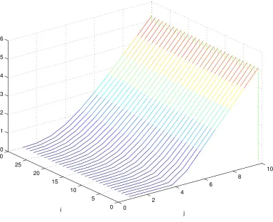
The MATLAB code forward.m in Listing 7.1 implements this method. In Figure 5, we show a Black–Scholes surface arising from this method. We used MATLAB’swaterfallplotting command to emphasize the timestepping nature of the finite difference iteration.

0

2

4

6

8

10

0 5 10 15 20 25 30

0 1 2 3 4 5 6

j i

Figure 5: Finite difference Black–Scholes surface fromforward.m.

Project Suggestions

• Speed up the code forward.m by replacing the matrix-vector multiplica-tions by vector operamultiplica-tions that access subarrays using MATLAB’s colon notation. (See [5, Chapter 5] for details of the colon notation.)

• Investigate the accuracy and stability of the explicit method inforward.m, and evaluate the improvements from (a) Crank–Nicolson and (b) upwinding for the ∂C/∂S term.

• Show that the binomial method may be regarded as a finite difference method and use this viewpoint to explain its convergence properties.

%FORWARD Forward Time Central Space on Black-Scholes PDE

% for European call

%

clf

%%%%%%% Problem and method parameters %%%%%%% E = 4; sigma = 0.5; r = 0.03; T = 1;

Nx = 11; Nt = 29; L = 10; k = T/Nt; h = L/Nx; %%%%%%%%%%%%%%%%%%%%%%%%%%%%%%%%%%%%%%%%%%%%%

T1 = diag(ones(Nx-2,1),1) - diag(ones(Nx-2,1),-1);

T2 = -2*eye(Nx-1,Nx-1) + diag(ones(Nx-2,1),1) + diag(ones(Nx-2,1),-1); mvec = [1:Nx-1]; D1 = diag(mvec); D2 = diag(mvec.^2);

Aftcs = (1-r*k)*eye(Nx-1,Nx-1) + 0.5*k*sigma^2*D2*T2 + 0.5*k*r*D1*T1;

U = zeros(Nx-1,Nt+1); Uzero = max([h:h:L-h]’-E,0); U(:,1) = Uzero; p = zeros(Nx-1,1);

for i = 1:Nt tau = (i-1)*k;

p(end) = 0.5*k*(Nx-1)*((sigma^2)*(Nx-1)+r)*(L-E*exp(-r*tau)); U(:,i+1) = Aftcs*U(:,i) + p;

end

waterfall(U’), xlabel(’j’), ylabel(’i’)

References

[1] T. A. Bass_{, The Predictors, Penguin, London, 1999.}

[2] F. Black and M. Scholes_{,The pricing of options and corporate liabilities,} Journal of Political Economy, 81 (1973), pp. 637–659.

[3] D. J. Higham_{, Nine ways to implement the binomial method for option} valuation in MATLAB, SIAM Review, 44 (2002), pp. 661–677.

[4] , An Introduction to Financial Option Valuation, Cambridge University Press, Cambridge, 2004, to appear.

[5] D. J. Higham and N. J. Higham_{, MATLAB Guide, SIAM, Philadelphia,} 2000.