Ewa M. Bednarz1,a, Amanda C. Maycock1,2,b, Paul J. Telford1,2, Peter Braesicke1,2,c, N. Luke Abraham1,2, and John A. Pyle1,2
1Department of Chemistry, University of Cambridge, Cambridge, UK 2National Centre for Atmospheric Science – Climate, Cambridge, UK anow at: Lancaster Environment Centre, Lancaster University, Lancaster, UK bnow at: School of Earth and Environment, University of Leeds, Leeds, UK
cnow at: Karlsruhe Institute of Technology, Institute for Meteorology and Climate Research, Karlsruhe, Germany
Correspondence:Ewa M. Bednarz ([email protected]) Received: 4 February 2018 – Discussion started: 26 February 2018
Revised: 27 November 2018 – Accepted: 3 December 2018 – Published: 17 April 2019
Abstract. The 11-year solar cycle forcing is recognised as an important atmospheric forcing; however, there remain un-certainties in characterising the effects of solar variability on the atmosphere from observations and models. Here we present the first detailed assessment of the atmospheric re-sponse to the 11-year solar cycle in the UM-UKCA (Uni-fied Model coupled to the United Kingdom Chemistry and Aerosol model) chemistry–climate model (CCM) using a three-member ensemble over the recent past (1966–2010). Comparison of the model simulations is made with satellite observations and reanalysis datasets. The UM-UKCA model produces a statistically significant response to the 11-year solar cycle in stratospheric temperatures, ozone and zonal winds. However, there are also differences in magnitude, spa-tial structure and timing of the signals compared to obser-vational and reanalysis estimates. This could be due to de-ficiencies in the model performance, and so we include a critical discussion of the model limitations, and/or uncertain-ties in the current observational estimates of the solar cy-cle signals. Importantly, in contrast to many previous stud-ies of the solar cycle impacts, we pay particular attention to the role of the chosen analysis method in UM-UKCA by comparing the model composite and a multiple linear regres-sion (MLR) results. We show that the stratospheric solar re-sponses diagnosed using both techniques largely agree with each other within the associated uncertainties; however, the results show that apparently different signals can be
identi-fied by the methods in the troposphere and in the tropical lower stratosphere. Lastly, we examine how internal atmo-spheric variability affects the detection of the 11-year solar responses in the model by comparing the results diagnosed from the three individual ensemble members (as opposed to those diagnosed from the full ensemble). We show overall agreement between the responses diagnosed for the ensemble members in the tropical and mid-latitude mid-stratosphere to lower mesosphere but larger apparent differences at North-ern Hemisphere (NH) high latitudes during the dynamically active season. Our UM-UKCA results suggest the need for long data sets for confident detection of solar cycle impacts in the atmosphere, as well as for more research on possible interdependence of the solar cycle forcing with other atmo-spheric forcings and processes (e.g. Quasi-Biennial Oscilla-tion, QBO; El Niño–Southern OscillaOscilla-tion, ENSO).
1 Introduction
using the UM-UKCA (Unified Model coupled to the United Kingdom Chemistry and Aerosol model) chemistry–climate model (CCM). Following recent improvements in the model, we present the first detailed analysis of the atmospheric im-pacts of the 11-year solar cycle simulated in UM-UKCA. In contrast to many previous solar cycle modelling studies in the literature, the novel approach we take is to pay partic-ular attention to the choice of detection method, comparing the model responses diagnosed using both a composite and a multiple linear regression (MLR) method. In addition we investigate how internal atmospheric variability affects the solar responses diagnosed in the model. Our results are par-ticularly relevant to understanding the potential sources of uncertainty in the estimated atmospheric impacts of the 11-year solar cycle forcing both in models (e.g. Mitchell et al., 2015a; Maycock et al., 2018) and observations and reanaly-ses (Mitchell et al., 2015b; Maycock et al., 2016).
The variation in solar spectral irradiance (SSI) as a func-tion of wavelength is important for determining the atmo-spheric response to the 11-year solar cycle. Given a typical change in total solar irradiance (TSI) over the 11-year so-lar cycle of ∼1 W m−2, the associated percentage irradiance variability in the visible and infrared parts of the spectrum is relatively small while the variability in the ultraviolet (UV) region is larger (Fig. S1 in the Supplement). According to the fifth Coupled Model Intercomparison Project (CMIP5) recommendations (http://solarisheppa.geomar.de/cmip5, last access: 26 August 2016, Lean, 2000; Wang et al., 2005; Lean, 2009), the SSI at ∼220–240 nm varies by ∼3 %–4 % and at∼180 nm by∼10 % (see Fig. S1). The SSI variability is even larger for wavelengths below 180 nm, which has impor-tant consequences for mesospheric O2absorption and
result-ing shortwave heatresult-ing there (Nissen et al., 2007). It is now well understood that stratospheric UV absorption by ozone increases stratospheric temperatures, while the radiation at wavelengths below∼242 nm is important for ozone produc-tion. This solar-cycle-induced ozone response provides an additional source of stratospheric heating (Haigh, 1994).
Solar-cycle-induced changes in stratospheric ozone over its 11-year cycle of between∼1 % and∼5 %–6 % have been reported from the analysis of various satellite (Soukharev and Hood, 2006; Tourpali et al., 2007; Dhomse et al., 2013, 2016; Maycock et al., 2016) and ground-based records (Tourpali et al., 2007). These, alongside changes in incoming solar UV radiation over the 11-year solar cycle, alter stratospheric tem-peratures (e.g. Gray et al., 2010). In the tropical upper strato-sphere, a temperature increase of∼0.7–1.1 K between solar maximum (SMAX) and minimum (SMIN) has been reported from rocketsonde and satellite data (Dunkerton et al., 1998; Ramaswamy et al., 2001; Keckhut et al., 2005; Randel et al., 2009; SPARC, 2010), with somewhat larger responses found in some reanalysis datasets (Frame and Gray, 2010; Mitchell et al., 2015b). In addition to the temperature and ozone re-sponses in the mid- and upper stratosphere, secondary max-ima have been identified in the tropical lower stratosphere,
which are often explained to be of dynamical origin (see be-low).
The most frequently invoked mechanism to explain how the direct solar-cycle-induced response in the upper strato-sphere can propagate down to the lower atmostrato-sphere and af-fect tropospheric climate is that first proposed by Kuroda and Kodera (2002) and Kodera and Kuroda (2002). In particu-lar, Kuroda and Kodera (2002) reported the development of a positive zonal wind anomaly in the subtropical upper strato-sphere for solar maximum during autumn in each hemistrato-sphere that is consistent with the strengthened horizontal tempera-ture gradient. In that study, the positive Northern Hemisphere (NH) zonal wind response developed and propagated pole-ward and downpole-ward during the course of early winter, ac-companied by a relative cooling of the polar stratosphere. These early winter anomalies were followed by opposite signed responses in late winter. The authors (see also Kodera and Kuroda, 2002) postulated that the initial strengthening of the vortex near the subtropical stratopause initiates a chain of dynamical feedbacks between atmospheric planetary waves and the zonal mean flow that modulates the strength of the stratospheric jet (thereby influencing an internal mode of high-latitude stratospheric variability), with reduced up-ward and equatorup-ward wave propagation associated with a stronger and colder polar vortex, and vice versa. This mech-anism was developed further by Kodera and Kuroda (2002), who also postulated that the solar-cycle-induced modulation of wave activity could impact on the large-scale Brewer– Dobson circulation (BDC), as manifested by the weakening of both the high-latitude downwelling and the tropical up-welling in early winter (and the opposite in late winter). The authors noted that this in turn would lead to adiabatic warm-ing and higher ozone levels in the tropical lower stratosphere in early winter, thereby accounting for the secondary temper-ature and ozone maxima observed in the region. It is plausi-ble that coupling between the tropical lower stratosphere and tropospheric convection could also play a role in producing solar responses in this region (e.g. Yoo and Son, 2016).
servations and model simulations, which can make it difficult to compare results between studies. Some authors composite data into bins representing periods of high and/or low solar cycle forcing (e.g. Kuroda and Kodera, 2002; van Loon et al., 2004; Chiodo et al., 2012; Matthes et al., 2013), while others use more complex statistical regression techniques (e.g. MLR) to account for the effects of different drivers (e.g:. Frame and Gray, 2010; Misios and Schmidt, 2013; Roy, 2014; Mitchell et al., 2015b; Hood et al., 2015; Maycock et al., 2016, 2018). Clearly, the use of a simpler compos-ite methodology increases the likelihood for the solar sig-nal to be contaminated with noise and/or the effects of other time-varying drivers, particularly in the case of small sample sizes. On the other hand, the MLR approach usually relies on the individual forcings being independent of one another and combining linearly, which might not be the case in a highly non-linear system like the atmosphere. The choice of analy-sis method was found to affect the derived surface responses to solar cycle (Roy and Haigh, 2010, 2012; Roy, 2014). An-other related factor regarding the uncertainty in atmospheric solar responses is the potential influence of internal atmo-spheric variability on the signal detection, which will again be more prominent in short records.
In this paper, following recent model improvements, we present the first detailed assessment of the atmospheric re-sponse to the 11-year solar cycle simulated by an ensemble of integrations performed with the UM-UKCA chemistry– climate model. We analyse the simulated atmospheric re-sponses to the 11-year solar cycle in UM-UKCA using both composite and MLR techniques, allowing a direct compar-ison of the methods. In order to understand potential lim-itations in deriving the solar-cycle-induced responses from records comparable in length to the current observations and reanalysis datasets, we analyse the solar cycle responses in the individual ensemble members and compare them. We note that another method for isolating the atmospheric solar cycle response in models is to use idealised time-slice inte-grations (e.g. Bednarz et al., 2018), but that approach is less comparable to the behaviour of the real atmosphere and is thus not considered here.
2 Methodology
2.1 The UM-UKCA model
2.1.1 The base chemistry–climate model
We use the UK Chemistry and Aerosol Model coupled to version 7.3 of the Met Office Unified Model (UM-UKCA) in the HadGEM3-A r.2.0 configuration (Hewitt et al., 2011). The configuration uses prescribed sea surface temperatures (SSTs) and sea ice. The horizontal resolution is 2.5◦latitude by 3.75◦ longitude, with 60 vertical levels up to ∼84 km. The time evolution of dynamical prognostic variables, with the exception of density, and the transport of chemical trac-ers is carried out within a semi-Lagrangian advection scheme described in Davies et al. (2005). The model includes param-eterised orographic and non-orographic gravity wave drag (Scaife et al., 2002; Webster et al., 2003) and simulates an in-ternally generated Quasi-Biennial Oscillation (QBO; Scaife et al., 2002).
The chemistry scheme used is the extended chemistry of the stratosphere scheme (CheS+, e.g. Bednarz et al., 2016). It follows from the standard stratospheric chemistry scheme (CheS) described in Morgenstern et al. (2009). However, un-like the lumping of all halogenated source gases into the three main species (CFCl3, CF2Cl2and CH3Br) employed in
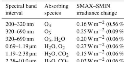
Table 1.Yearly mean irradiance change between the years 1981 and 1986 (1TSI=1.06 W m−2) for each of the UM-UKCA shortwave heating bands.
Spectral band Absorbing SMAX–SMIN interval species irradiance change
200–320 nm O3 0.16 W m−2(0.56 %)
320–690 nm O3 0.25 W m−2(0.09 %)
320–690 nm O3, H2O 0.20 W m−2(0.06 %)
0.69–1.19 µm H2O, O2 0.27 W m−2(0.06 %)
1.19–2.38 µm H2O, CO2 0.15 W m−2(0.06 %)
2.38–10.0 µm H2O, CO2 0.03 W m−2(0.06 %)
et al., 2010). The emissions of ozone-depleting substances (ODSs) as well as of CH4, N2O and H2 are accounted for
using lower boundary concentrations. The model-calculated concentrations of O3, N2O, CH4, CCl3F, CCl2F2, C2Cl3F3
and CHClF2 are coupled to the radiation scheme; the
spe-cific humidity field from the physical model and prescribed CO2concentrations are also used by the radiative scheme.
2.1.2 The representation of the 11-year solar cycle in UM-UKCA
The 11-year solar cycle variability has been implemented in UM-UKCA in both the radiation and photolysis schemes. This is an advance on earlier version of the model that did not include solar cycle variability (see for example SPARC, 2010). The method for implementing the solar cycle forc-ing in the shortwave radiation scheme follows that in the HadGEM1 (Stott et al., 2006) and HadGEM2-ES models (Jones et al., 2011). The model’s radiation scheme (Ed-wards and Slingo, 1996) has six spectral bands from 200 nm to 10.0 µm (Table 1) in the shortwave spectral region. The yearly mean TSI data used are those recommended for the CMIP5 simulations (Fröhlich and Lean, 1998; Lean, 2000; Wang et al., 2005; Lean, 2009), post-processed to constrain the mean over 1700–2004 to 1365 W m−2 (Jones et al., 2011). A fit to spectral data from Lean (1995) is used to account for the change in partitioning of solar ra-diation into wavelength bins. Table 1 shows how the TSI change of 1.06 W m−2, i.e. the difference between the years 1981 (solar maximum) and 1986 (solar minimum), is par-titioned into the individual bands of the model’s shortwave radiation scheme. Using this parameterisation, the irradi-ance in the main UV band (200–320 nm) increases during SMAX by∼0.16 W m−2(0.56 %). Note that this is∼20 %
smaller than the corresponding 200–320 nm spectral irradi-ance change between these two years (∼0.20 W m−2) rec-ommended in the more recent CMIP5 SSI specifications (Lean, 2000; Wang et al., 2005; Lean, 2009).
In the Fast-JX photolysis scheme, the change in partition-ing of solar irradiance into wavelength bins is accounted for by scaling the irradiance in the 18 photolysis bins according
to the difference in the yearly mean CMIP5 SSI data for the years 1981 (SMAX) and 1986 (SMIN) (see Fig. S1b) and the long-term evolution of TSI. As noted above, the Fast-JX scheme is used only for wavelengths between 177 and 850 nm. At pressures less than 0.2 hPa, i.e. where photolysis rates are calculated using the lookup tables, the 11-year solar cycle variability is reflected in the TSI change only, with no modulation of the spectral distribution of solar irradiance. 2.2 The UM-UKCA experiments
A three-member ensemble of transient integrations covering 1960–2010 was performed. The first 6 years of each simu-lation were treated as spin-up and, therefore, only the 1966– 2010 period is analysed below. With the exception of the new implementation of solar cycle variability in the model, the experimental set-up is identical to the UM-UKCA integra-tion shown in the recent SPARC report on theLifetimes of Stratospheric Ozone-Depleting Substances, Their Replace-ments, and Related Species(SPARC, 2013; Chipperfield et al., 2014). The prescribed SSTs and sea ice follow observa-tions (Rayner et al., 2003). Greenhouse gases (GHGs) fol-low the SRES A1B scenario (IPCC, 2000) and ODSs folfol-low WMO (2011). The sulfate surface area density (SAD) field recommended for the Chemistry-Climate Model Validation 2 (CCMVal2) models (SPARC, 2006; Eyring et al., 2008; Morgenstern et al., 2010) is prescribed in the stratosphere for the heterogeneous reactions on aerosol surfaces. As with previous versions of UM-UKCA, the coupling of SAD with the photolysis and radiation schemes is not included in this model version.
2.3 The observation and reanalysis datasets
Observed estimates of the temperature and zonal wind re-sponses to the solar cycle forcing are derived from the ERA-Interim (ERAI) reanalysis (Dee et al., 2011). We note that the existence of artificial jumps in the upper stratospheric tem-perature record, which can influence the diagnosed solar cy-cle response (see for example Hood et al., 2015; Mitchell et al., 2015b), was corrected prior to the analysis following the procedure described in McLandress et al. (2014). Although we use only one reanalysis dataset here for comparison with the model, it is important to note that there are quantitative differences in the diagnosed stratospheric responses to solar forcing amongst various current reanalyses (Mitchell et al., 2015b).
Figure 1.Time series of anomalies in TSI (W m−2) from the orig-inal CMIP5 recommendations (blue; http://solarisheppa.geomar. de/cmip5, last access: 16 April 2015; Fröhlich and Lean, 1998; Lean, 2000; Wang et al., 2005; Lean, 2009), TSI (W m−2) as given by the processed CMIP5 recommendations imposed in UM-UKCA (green; Fröhlich and Lean, 1998; Lean, 2000; Wang et al., 2005; Lean, 2009; Jones et al., 2011) and the F10.7 cm radio flux (SFU) (red; http://lasp.colorado.edu/lisird/tss/noaa_radio_flux. html, last access: 30 April 2015). SMAX and SMIN years used in the composite methodology are highlighted in magenta and yellow, respectively.
al., 2015). We use the units of ozone number density, as op-posed to volume mixing ratios, in order to avoid uncertainties associated with the choice of temperature record used for the conversion (e.g. Maycock et al., 2016; Dhomse et al., 2016). 2.4 The analysis methods
We use two statistical methods for isolating the atmospheric response to the solar cycle forcing. The first is a simple com-posite methodology (henceforth referred to as “comcom-posites”). Data from each ensemble member are linearly detrended and 3 years of data per each SMAX and SMIN are chosen based on the three highest and three lowest yearly mean TSI val-ues in each∼11-year cycle (Fig. 1). This gives 12 years of SMAX and 12 years of SMIN per ensemble member, result-ing in 36 SMAX and 36 SMIN years for the full ensemble. A mean SMAX–SMIN difference is calculated and its magni-tude scaled to represent a response per 1 W m−2of the TSI.
The second method is a multiple linear regression tech-nique. The MLR code is the same as that used and de-scribed in SPARC (2010), with a similar method also used in Bodeker et al. (1998) and Kunze et al. (2016). In this case, the time evolution of a variable,y(t ), can be defined as
and is defined as the global monthly mean Cly+60·Bry
at 20 km, as was done in SPARC (2010) following New-man et al. (2007). Cly and Bry denote total inorganic
here. In addition, when tested on the simulated zonal mean zonal wind and temperature data the approach was found to result in locally slightly higherR2values for some of the in-dividual months thanR2for the individual months calculated with the Fourier expansion described above (not shown). An example of a resulting fit and a residual is shown in Fig. S2.
In order to estimate the statistical significance of the de-rived regression coefficients, the first MLR calculation is fol-lowed by a transformation of the regression model (Markus Kunze, personal communication, 2012; Tiao et al., 1990; Bodeker et al., 1998; SPARC, 2010). In particular, a second-order autoregressive model for the residuals is used (Eq. 2): R(t )=ρ1R(t−1)+ρ2R(t−2)+a(t ), (2)
whereρ1andρ2are regression parameters anda(t )is a
ran-dom variable. The fitted values ofρ1andρ2are used to
trans-form the input basis functions and the input variable y(t ), and the MLR is performed again to yield the associatedt -test statistics and/ort-test probabilities.
In order to derive solar regression coefficients from the full ensemble, the model output and basis functions from each of the three ensemble members were concatenated into a 135-year-long time series and the MLR was performed using the combined datasets. A similar approach has been adopted in Gray et al. (2013) and Hood et al. (2013).
For consistency with the model, the MLR analysis of ERAI and SAGE II data also employs TSI as the regressor for the solar cycle forcing. However, unlike the yearly mean TSI time series that forces the model, the time series chosen here is that originally recommended for the CMIP5 models (http: //solarisheppa.geomar.de/cmip5, last access: 16 April 2015; Fröhlich and Lean, 1998; Lean, 2000; Wang et al., 2005; Lean, 2009, Fig. 1), varying on a monthly basis. We note that a number of proxies for solar forcing have been used in the literature (see Gray et al., 2010, for details), with one of the most common being the 10.7 cm solar radio flux (F10.7). Fig-ure 1 (blue and red curves) illustrates that there is a good de-gree of correlation between the TSI and F10.7 proxies, in par-ticular on longer timescales (R=0.81, with 1 W m−2=101 (±8) solar flux units, SFU).
For simplicity, the observed solar responses in ERAI and SAGE II discussed here are derived from MLR only. In this case, the volcanic regressor used, SAD(t), is the same as in the model. The QBO(t), QBO_orth(t) and ENSO(t) were calculated in the same way as in the model but us-ing the ERAI zonal wind and SST data (Dee et al., 2011). ESC(t) is replaced with EESC(t) (equivalent effective strato-spheric chlorine), which estimates stratostrato-spheric Clyand Bry
from their tropospheric source gases, here assuming the at-mospheric circulation with the age of air spectrum with the mean of 3 years (as was done in SPARC, 2010, following Newman et al., 2007). The MLR analysis is performed over 1979–2008 for ERAI and over October 1984 to August 2005 for SAGE II.
3 The ensemble yearly mean response in UM-UKCA This section focuses on the yearly mean atmospheric re-sponse to the 11-year solar cycle forcing simulated in the ensemble of the transient UM-UKCA integrations. In par-ticular, the yearly mean changes in shortwave heating rates, temperature, ozone and zonal wind from the combined en-semble are discussed; the model responses are derived using both MLR and composites and, where available, compared with the reanalysis or observations.
3.1 Shortwave heating rates
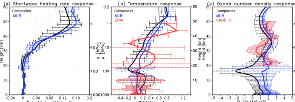
Figure 2a shows the yearly mean tropical mean (25◦S– 25◦N) shortwave heating rate response to the 11-year solar cycle forcing in the UM-UKCA model, expressed as a re-sponse per W m−2change in TSI. The response maximises in the tropical stratopause region, reaching up to∼0.16 and 0.14 K day−1W−1m2for the MLR and composite methods,
respectively. Notably, this solar-cycle-induced modulation constitutes a relatively small fraction of the absolute short-wave heating rates in this region (∼1.5 % near 50 km). The magnitude of the MLR-derived maximum is somewhat larger than in the composites, although the two are not significantly distinguishable, in a statistical sense, given the estimated un-certainties in each.
3.2 Temperature and zonal winds
3.2.1 The tropical upper stratospheric temperature response
The corresponding yearly mean tropical temperature re-sponse to the solar cycle forcing is shown in Fig. 2b, compared with the ERAI reanalysis. The MLR tropical temperature response in UM-UKCA maximises above the stratopause at∼0.8 K W−1m2. In comparison, the tropical mean ERAI response maximises in the upper stratosphere at ∼1–1.1 K W−1m2(in agreement with previous ERAI stud-ies, e.g. Mitchell et al., 2015b; Hood et al., 2015; Kodera et al., 2016). Compared to ERAI the UM-UKCA-simulated temperature maximum thus occurs at higher altitudes and is ∼25 % smaller.
Figure 2. Yearly mean zonal mean(a)shortwave heating rate (K day−1W−1m2),(b) temperature (K W−1m2) and(c)ozone number density (% W−1m2) responses to the 11-year solar cycle forcing in the tropics (25◦S–25◦N) in UM-UKCA. The UM-UKCA responses were derived using composites (black) and MLR (blue). Shown also in red are the corresponding ERAI MLR temperature(b)and SAGE II MLR ozone(c)responses. The error bars denote the corresponding confidence intervals, represented here by±2 standard errors of the mean response.
the wavelengths higher than 200 nm excludes changes in the mesospheric absorption by oxygen near the Lyman-α line (121.6 nm), where percentage irradiance changes during the solar cycle can be particularly large (Lean, 2000; Nissen et al., 2007).
Another factor that is likely to be important for the magni-tude of the upper stratospheric temperature response is the fact that the model has used a relatively modest modula-tion of SSI. There has been considerable uncertainty associ-ated with the solar cycle modulation of SSI due to the short-age of long-term satellite measurements, with marked differ-ences between the individual available datasets (e.g. Harder et al., 2009; Dhomse et al., 2013; Ermolli et al., 2013). We also note that whilst being consistent with the design of the HadGEM2-ES model (Jones et al., 2011), the current imple-mentation of the solar cycle forcing in the model’s radiation scheme results in an underestimation of the UV changes in the 200–320 nm band by around ∼20 % compared to the CMIP5 SSI recommendations (Sect. 2.1.2).
Lastly, there are large uncertainties in the reanalysis datasets in the upper stratosphere due to the scarcity of long-term measurements (McLandress et al., 2014; Long et al., 2017). As a result, large differences exist between reanaly-ses in both the structure and magnitude of the upper strato-spheric/lower mesospheric temperature response to the solar cycle (Mitchell et al., 2015b). A somewhat smaller tempera-ture response was estimated from the stratospheric sounding unit satellites (SPARC, 2010; Randel et al., 20091), although
1Up to ∼0.6–0.7 K per 100 SFU, SPARC (2010); up to ∼
1 K per 125 SFU, Randel et al. (2009). Recall that 1 W m−2≈ 100 SFU, Sect. 2.4.
this could be related to their relatively poor vertical resolu-tion (Gray et al., 2009).
We note that even models forced with identical SSI vari-ations still show relatively broad ranges of solar cycle tem-perature responses (e.g. Austin et al., 2008; SPARC, 2010; Mitchell et al., 2015a). SPARC (2010) showed that model performance in simulating the direct radiative response to a change in solar irradiance alone could not fully account for the spread of simulated temperature responses, suggest-ing some contribution of indirect dynamical processes. This aspect will be investigated further in Sect. 6, where the so-lar response found from the individual ensemble members is considered. Lastly, the differences in stratospheric temper-ature responses could be related to solar ozone responses, which is discussed in Sect. 3.3.
3.2.2 The tropical lower stratospheric temperature response
anoma-lies were found in UM-UKCA (Fig. 4b). Instead, the yearly mean UM-UKCA-simulated response is dominated by the regions of a relative zonal wind deceleration. Therefore, any strengthening of the stratospheric vortex and the associated reduction in the large-scale circulation in UM-UKCA is too weak and/or short lived to have an impact on the tropical upwelling that would be visible in the yearly mean. Possibly, the coupling of the ocean and tropical convection, which may also play a role in influencing the tropical lower stratosphere (e.g. Yoo and Son, 2016), is also not adequately represented in the model set-up with prescribed (although observation-ally derived) SSTs. In the case of the Northern Hemisphere, a more detailed seasonal analysis of the simulated dynamical response is presented in Sect. 4.
One challenge for attributing signals in the tropical lower stratosphere is possible aliasing between the effects of solar forcing with other natural forcings and processes, e.g. vol-canic forcing, QBO or ENSO (e.g. Lee and Smith, 2003; Marsh and Garcia, 2007; Smith and Matthes, 2008; Chiodo et al., 2014; Mitchell et al., 2015b). Chiodo et al. (2014) used the WACCM (Whole Atmosphere Community Climate Model) model and found that the secondary tropical tem-perature maximum widely attributed to the 11-year solar cy-cle over the reanalysis period largely disappeared if volcanic eruptions were not included in the model. In this version of UM-UKCA the stratospheric aerosols are coupled only to the heterogeneous chemistry scheme and not to the photoly-sis or radiative heating schemes; the relative overlap between the elevated values of the aerosol SAD index following the main volcanic eruptions and the years selected as compos-ite SMAX years is also relatively small here (not shown). Therefore if aliasing with volcanic eruptions was an impor-tant contributor to the lower stratospheric temperature max-imum in reanalysis, this effect would not be reproduced in UM-UKCA.
3.2.3 The mid-latitude troposphere
In the troposphere, ERAI shows a small warming (∼0.1– 0.2 K W−1m2) in the mid-latitudes on both hemispheres (Fig. 3c), accompanied by a weakening of the extratropical zonal winds at ∼30◦ in the troposphere and lower strato-sphere alongside somewhat weaker opposite sign responses in the mid-latitudes (Fig. 4c). These tropospheric dipole pat-terns represent a weakening and poleward shift of the mid-latitude jets and an associated expansion of the Hadley circu-lation (Haigh et al., 2005; Haigh and Blackburn, 2006).
In agreement with ERAI, UM-UKCA simulates a statis-tically significant warming of up to∼0.2 K W−1m2in the NH mid-latitude troposphere, detectable for both analysis methods (Fig. 3a, b). This is accompanied by a weakening of the NH extratropical zonal wind (MLR), which is broadly similar to ERAI albeit smaller in magnitude and without a strong accompanying westerly response in the mid-latitudes (Fig. 4a, b). Interestingly, the modulation of the NH
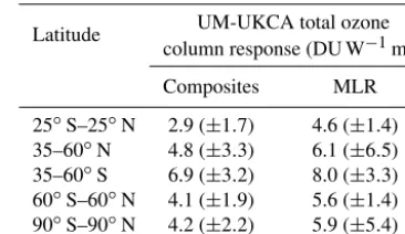
subtropi-Table 2.Yearly mean total ozone column response (DU W−1m2), ±2 standard errors, in UM-UKCA derived using composites and MLR.
Latitude UM-UKCA total ozone column response (DU W−1m2) Composites MLR
25◦S–25◦N 2.9 (±1.7) 4.6 (±1.4) 35–60◦N 4.8 (±3.3) 6.1 (±6.5) 35–60◦S 6.9 (±3.2) 8.0 (±3.3) 60◦S–60◦N 4.1 (±1.9) 5.6 (±1.4) 90◦S–90◦N 4.2 (±2.2) 5.9 (±5.4)
cal jet in UM-UKCA occurs in the absence of a strong yearly mean tropical warming in the lower stratosphere, which has been shown to be a driver of the tropospheric wind re-sponses (Haigh et al., 2005; Simpson et al., 2009) and/or strong yearly mean stratospheric westerly anomalies. How-ever, Misios and Schmidt (2013) showed that a weakening and poleward shift of the subtropical jets that project onto the timescale of the solar cycle forcing could be reproduced in a model forced only with the prescribed observationally derived SSTs and sea ice. It is therefore plausible that the solar signal, or other variability, found in the prescribed ob-served SSTs could contribute to the diagnosed tropospheric wind changes in UM-UKCA. We note, however, that unlike the hemispherically symmetric tropospheric zonal wind and temperature response in ERAI, UM-UKCA does not capture such poleward shift of the yearly mean tropospheric jet or a mid-latitude warming in the SH. The role of prescribed SSTs in the diagnosed solar cycle response is further discussed in Sect. 6 in the context of the solar responses found in the in-dividual ensemble members.
3.3 Ozone
3.3.1 Total ozone column
The UM-UKCA MLR results show a yearly mean global mean total column ozone response of around ∼ 6 DU W−1m2(Table 2). In comparison, total column ozone responses over the solar cycle of a few DU in the tropics and mid-latitudes have also been reported from observations (Randel and Wu, 2007; SPARC, 2010; Lean, 2014), but with some differences between the individual datasets or their dif-ferent versions (Randel and Wu, 2007; Lean, 2014).
3.3.2 The tropical/mid-latitude stratosphere
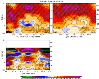
[image:8.612.337.520.109.215.2]Figure 3.Yearly mean zonal mean temperature response (K W−1m2) in UM-UKCA derived using composites(a)and MLR(b), as well as in ERAI derived using MLR(c). Shading indicates statistical significance on the 95 % level (ttest). Contour spacing is 0.1 K W−1m2.
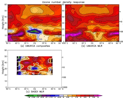
also Soukharev and Hood, 2006; Randel and Wu, 2007; Gray et al., 2009; Dhomse et al., 2013, 2016; Maycock et al., 2016) and is more uniform over the mid-stratosphere com-pared to the more peaked structure in the upper stratosphere in SAGE II. It also maximises at lower levels than in the ob-servations (Figs. 2c and 5). The relatively lower altitude of the tropical ozone maximum compared to satellite observa-tions is a common feature amongst various CCMs (Maycock et al., 2018). We note that differences exist between the mag-nitudes as well as the structures of the ozone responses found in different satellite products and/or their different versions (Soukharev and Hood, 2006; Dhomse et al., 2013, 2016; Maycock et al., 2016).
The lower altitude of the maximum ozone response in UM-UKCA compared to observations could contribute to the lower magnitude of the tropical temperature response. As noted in Sect. 3.2.1, there are large differences between the different SSI datasets (e.g. Ermolli et al., 2013) and the UM-UKCA model is forced with relatively modest modulation of SSI at the lower end of the current estimates. Yet, the recent sensitivity study in Maycock et al. (2018) suggested a CCM forced with larger SSI variability would also produce a
max-imum tropical ozone response to solar forcing at a relatively lower altitude than in satellite observations. The relatively lower altitude of the UM-UKCA model response could also arise due to model deficiencies, e.g. in the photolysis code, and/or uncertainties in the observed response. Regarding the performance of the model photolysis code, Sukhodolov et al. (2016) found a small (∼0.2 %–0.3 %) underestimation of the ozone response to the solar cycle in the upper strato-sphere in the Fast-JX code used in UM-UKCA compared with line-by-line calculations2; this gave rise to only a small temperature underestimation of∼0.05 K. Thus, it appears that the details of the model photolysis scheme alone can-not explain the apparent differences in the simulated tropi-cal upper stratospheric ozone response compared to SAGE II measurements. With respect to observational uncertainties, it is important to understand that our chemistry–climate model simulates, by definition, an ozone response to the solar cy-cle forcing that is consistent with the imposed SSI varia-tion and the associated changes in temperature and
trans-2For the solar cycle variability given by COSI SSI, represented
Figure 4.As in Fig. 3 but for the zonal mean zonal wind response (m s−1W−1m2). Contour spacing is 0.2 m s−1W−1m2; note also the additional contour at±0.1 m s−1W−1m2.
port. The modelled impact on stratospheric temperatures of the increased ozone levels under higher solar cycle activity will thus inevitably differ from that simulated by general cir-culation models that use prescribed observationally derived ozone changes (Maycock et al., 2018). The role of the repre-sentation of the solar–ozone feedback is discussed in detail using specially designed sensitivity experiments in Bednarz et al. (2019).
4 The ensemble NH seasonal response in UM-UKCA 4.1 Temperature and zonal wind
The previous section analysed the yearly mean zonal wind and temperature responses to the 11-year solar cycle simu-lated in UM-UKCA. The following section presents an anal-ysis of the seasonal evolution of the diagnosed responses with a focus on the NH winter season. Figure 6 shows the November–April monthly mean NH temperature responses in both UM-UKCA and ERAI, and Fig. 7 shows the associ-ated monthly mean changes in zonal wind.
4.1.1 The ERAI reanalysis
ob-Figure 5.Yearly mean zonal mean ozone number density response (% W−1m2) in UM-UKCA derived using composites(a)and MLR(b), as we all as in SAGE II derived with MLR(c). The percentages are calculated relative to the mean over the 1966–2010(a, b)and 1985– 2004(c)periods. Hatching in(a, b)as in Fig. 3. The thick white line in(c)encompasses regions where the statistical significance exceeds the 95 % confidence level. Contour spacing is 0.5 % W−1m2up to±7 % W−1m2.
served solar response over a relatively short time period (see also Sect. 6). In the tropical lower to mid-stratosphere (100– 10 hPa), there is a region of warming between November and January, which contributes to the yearly mean secondary temperature maximum discussed in Sect. 3.2.
Later in February, the strengthening and cooling of the stratospheric vortex in ERAI is replaced by a stronger and statistically significant response of opposite sign. The Febru-ary sign reversal has been found to be a robust feature of the various reanalysis data sets available (e.g. Matthes et al., 2004; Frame and Gray, 2010; Hood et al., 2015; Mitchell et al., 2015b; Kodera et al., 2016). Despite the sign reversal in the mid- and high latitudes, the westerly zonal wind anomaly near the subtropical stratopause persists throughout the win-ter into spring. It then amplifies and descends down to the stratosphere and troposphere in April, accompanied by an anomalous high-latitude cooling (where it persists at reduced magnitude until∼June, not shown; see also Mitchell et al., 2015b). As pointed out by Mitchell et al. (2015b), despite the robustness of the response, these springtime anomalies have
largely been ignored in the literature. In general, the ERAI results shown here agree with the previous reanalysis studies (e.g. Matthes et al., 2004; Frame and Gray, 2010; Mitchell et al., 2015b; Hood et al., 2015; Kodera et al., 2016).
4.1.2 The UM-UKCA model
The UM-UKCA results in November show a qualitatively similar but weaker pattern of temperature changes to ERAI consisting of a relative warming in the tropical upper strato-sphere and lower mesostrato-sphere (up to∼1 K W−1m2) and a cooling in the polar region (of up to∼1.5–2.5 K W−1m2).
[image:11.612.89.509.65.397.2]Figure 6.Monthly mean November–April zonal mean temperature response (K W−1m2) in UM-UKCA derived using MLR(a)and com-posites(b). Shown also is the ERAI response derived with MLR(c). Single and double hatching indicates statistical significance on the 90 % and 95 % level, respectively (ttest). Note the additional contours at±0.25 K W−1m2.
and is weaker than the larger and more localised response in ERAI (November–January).
In December, both the temperature and zonal wind re-sponses simulated in UM-UKCA weaken compared to November. While some cooling remains in the polar lower stratosphere, an opposite sign response develops in the up-per stratosphere aloft. In midwinter (January–February), the polar warming magnifies and descends, alongside the sim-ulated weakening of the stratospheric jet. While the easterly anomaly propagates down through the lower mesosphere and stratosphere, the westerly response redevelops near the sub-tropical stratopause. It then appears to propagate poleward and, to some extent, down in the stratosphere in spring, re-versing sign in April. However, the anomalies derived from MLR and composite analysis are not highly statistically sig-nificant in April, suggesting a small signal-to-noise level. 4.1.3 Discussion
The evolution of the solar cycle response in the NH high lat-itudes in winter in UM-UKCA shows a shift in the timing of the UM-UKCA-modelled responses towards earlier in the
mid-Figure 7.As in Fig. 6 but for the zonal mean zonal wind change (m s−1W−1m2). Note the additional contours at±0.5,±8,±9 and ±10 m s−1W−1m2.
to late springtime (April onwards) stratosphere. Regarding the temperature anomalies simulated in the tropical lower stratosphere, while there is some general warming through-out the tropical stratosphere in UM-UKCA in November (i.e. when the largest westerly anomaly occurs in the mid- to high-latitude stratosphere), the temperature increase in the tropical lower stratosphere is very small and does not form a distinct maximum as in ERAI.
The differences in the timing of the UM-UKCA-modelled zonal wind and temperature responses compared with the reanalysis could be related to a positive bias in the back-ground zonal wind climatology in UM-UKCA (not shown). As pointed out by Kodera and Kuroda (2002), the mechanism behind the high-latitude response to the solar cycle forcing relies on the non-linear interactions between the planetary waves and the mean flow and, therefore, is influenced by the climatological mean state. It is well known that the propa-gation of planetary waves through the mid- and high-latitude stratosphere is strongly dependent on the strength and direc-tion of the background zonal wind, with the planetary waves propagating only if the winds are westerly and not too strong (Charney and Drazin, 1961; Andrews et al., 1987). The
im-portance of a realistic climatology in models for reproduc-ing the observed dynamical response to the solar cycle forc-ing has also been suggested by other studies, e.g. Kodera et al. (2003), Matthes et al. (2004), Rind et al. (2008), Schmidt et al. (2010) and Chiodo et al. (2012). The differences in tim-ing could also be related to errors in the prescribed SSI forc-ing in UM-UKCA, which may not be representative of the true SSI variability (Ermolli et al., 2013).
4.2 Mechanism
[image:13.612.49.549.67.396.2]Figure 8. Monthly mean November–April scaled EP flux divergence (i.e. (∇ ·F)/(ρ·a·cosφ); see Andrews et al., 1987) response (m s−1day−1W−1m2) in UM-UKCA derived with MLR. Single and double hatching indicates statistical significance on the 90 % and 95 % level, respectively (ttest). Contour spacing is 0.3 m s−1day−1W−1m2.
The changes in zonal mean circulation simulated in UM-UKCA discussed above are associated with consistent changes in wave propagation and breaking. In particular, the development of the positive zonal wind response to higher solar cycle forcing in autumn (November, Fig. 7) is as-sociated with a decreased propagation of planetary waves through the stratosphere (not shown) and a reduction in wave breaking throughout the mid- and high-latitude stratosphere and lower mesosphere (divergence of Eliassen–Palm, EP, flux of up to∼2.5 m s−1day−1W−1m2, Fig. 8). This reduc-tion in the deposireduc-tion of eddy heat and momentum acceler-ates the zonal wind, which should feed back on planetary waves and result in even less wave propagation and break-ing. So, there is a two-way interaction between the waves and zonal wind, as also discussed in Kuroda and Kodera (2002), Kodera and Kuroda (2002), Matthes et al. (2004, 2006) and Chiodo et al. (2012).
Later in December and January, UM-UKCA simulates an increase in the mid-/high-latitude wave propagation (not shown) and increased wave breaking under higher solar cy-cle forcing in December and January, which is particularly evident in the upper stratosphere and lower mesosphere (see the negative divergence of EP flux, i.e. convergence, of up to∼3.5–4 m s−1day−1W−1m2, Fig. 8). As this decelerates the zonal wind, the results are consistent with the consider-able weakening of the westerly zonal wind response in
De-cember, compared to November, and its sign reversal in Jan-uary. In the subtropics, the emergence of a positive zonal wind anomaly near the stratopause in January is associated with the region of a relative EP flux divergence that devel-ops over the mid- and high latitudes in February, consistent with the strengthening of the subtropical westerly signal in that month and its apparent poleward and downward prop-agation in March. However, the amplitudes of the EP flux divergence anomalies in late winter and early spring are gen-erally smaller than earlier and not highly statistically signifi-cant.
Figure 9. As in Fig. 8 but for the transformed vertical component of the residual circulation (w∗; see Andrews et al., 1987) response (mm s−1W−1m2) in UM-UKCA. Positive values indicate upwelling. Note the additional contours at±0.025 mm s−1W−1m2.
the mid-latitudes, possibly indicating a relative shift in the downwelling region towards the extratropics. In December and January, the sign of the model responses reverses
Thus, the UM-UKCA-simulated changes in planetary wave breaking andw∗in the high-latitude stratosphere agree with the postulated mechanism (Kuroda and Kodera, 2002; Kodera and Kuroda, 2002), albeit with some differences in the timing of the responses, as well as with the modelling results of Matthes et al. (2004) and Chiodo et al. (2012). Regarding the tropical lower stratosphere, while some in-dications of solar-cycle-induced upwelling and temperature anomalies that are consistent in terms of a sign with the BDC changes in the Arctic region are found, the magnitudes of the UM-UKCA tropical upwelling (and temperature) anomalies are very small in the lower stratosphere and not strongly sta-tistically significant, indicating that the mechanism is not ro-bustly reproduced in the model.
5 The role of detection method: composites vs. MLR Here we compare the UM-UKCA responses diagnosed by the composite and MLR methods. Model- and reanalysis-based studies in the published literature have adopted both of these methods but they are rarely applied together. The application of both methods to the same model simulations enables a clean comparison of the diagnosed responses.
5.1 Ensemble yearly mean temperature and zonal wind response
A comparison between the UM-UKCA tropical tempera-ture responses derived using composites and MLR shows a good agreement between the magnitudes of the detected up-per stratospheric/lower mesospheric temup-perature responses (Fig. 3). However, unlike the weak positive MLR tempera-ture response in the tropical lower stratosphere, composites yield a small statistically insignificant cooling of up to 0.2– 0.3 K W−1m2in that region. This is likely to be a manifes-tation of contributions from other forcings that affect lower stratospheric temperatures (e.g. QBO, ENSO) and interan-nual variability. Interestingly, in the troposphere, while no significant temperature response was detected with MLR in the tropics, composites yield a small, albeit locally statisti-cally significant,warming of up to∼0.2 K W−1m2. A large part of this temperature dipole structure seen in composites in the tropical troposphere/lower stratosphere is attributed to the residual term in our MLR analysis, with smaller contri-butions from the influence of ENSO and QBO (see Sect. S1 and Fig. S3).
from the solar component in the MLR analysis (Sect. S1 and Fig. S4). In the troposphere, the UM-UKCA compos-ites suggest an equatorward shift of the SH subtropical jet and a weakening of the polar night jet extending down to the surface at ∼60◦S, in qualitative agreement with ERAI (MLR). In contrast, no significant tropospheric response in the SH was found in UM-UKCA using MLR analysis. As with the tropospheric temperature response, the apparent dis-crepancy between the MLR and composite responses in the troposphere is related to the fact that parts of the latter are at-tributed to the residual and, to a smaller extent, ENSO terms in the MLR model (Sect. S1 and Fig. S4).
Assuming that the individual forcings are indeed com-pletely independent from each other and linear, the results suggest that MLR achieves a better level of separation of contributions from other processes and interannual variabil-ity not directly related to the solar forcing, therefore minimis-ing the effects of aliasminimis-ing and noise. However, the impacts of individual forcings may not necessarily be independent from one another and additive. A number of studies suggested that coupling of the solar cycle forcing with, for example, QBO and/or ENSO could be important (e.g. Salby and Callaghan, 2000; Pascoe et al., 2005; Labitzke et al., 2006; Haigh and Roscoe, 2006, 2009; Roscoe and Haigh, 2007; Camp and Tung, 2007; Kuroda, 2007; Lu et al., 2009; Calvo and Marsh, 2011; Roy and Haigh, 2011; Matthes et al., 2013). Therefore, we refrain here from judging unambiguously which tech-nique performs better in the detection of the solar responses. More importantly, we stress that the differences between the composite and MLR responses found in the troposphere and in the tropical lower stratosphere, although not statistically significant, illustrate that the use of only one of these tech-niques could lead to somewhat different conclusions with re-gard to the solar cycle response and, therefore, highlight that care needs to be taken when analysing solar responses in this region.
5.2 Ensemble yearly mean ozone response
Regarding the yearly mean ozone responses in the full en-semble, we find that the total column ozone responses de-rived in various regions are somewhat higher for MLR than for composites but agree to within the estimated uncertainty ranges (Table 2). Similarly, the spatial patterns of the MLR and composite ozone responses generally agree with each other in a large part of the stratosphere. The main differ-ences (albeit still not statistically significant) occur in the tropical stratosphere. In the lower stratosphere, in contrast to the weak positive MLR response, the composites suggest an ozone decrease of up to ∼3 % W−1m2–3.5 % W−1m2, consistent with the small temperature decrease found in that region (Fig. 4). As with the temperature and zonal winds, aliasing with other natural forcings could contribute to the tropical lower stratospheric ozone changes diagnosed in the composites, as suggested by the studies of for example Lee
and Smith (2003), Marsh and Garcia (2007), Smith and Matthes (2008), and Mitchell et al. (2015b).
5.3 Ensemble NH seasonal response
In general, the monthly mean NH high-latitude tempera-ture and zonal wind responses in UM-UKCA derived using composites and MLR during winter and spring are found to be qualitatively and quantitatively similar within the associ-ated uncertainties (Figs. 6 and 7), with somewhat stronger and more significant strengthening of the tropospheric zonal wind at∼60◦N found from composites in November.
6 Solar cycle response over the recent past in the individual ensemble members
Uncertainties exist regarding the atmospheric response to the 11-year solar cycle forcing. So far, we have focused on the solar cycle response in UM-UKCA across all three ensemble members for the recent past combined. However, observa-tional and reanalysis records such as ERAI or SAGE II repre-sent only a single realisation of the real atmosphere. In order to gain knowledge about underlying variability and, there-fore, understand potential issues in deriving solar responses from records comparable in length to the current observa-tions and reanalysis dataset, it is informative to examine the solar responses simulated in each individual ensemble mem-ber separately.
The annual mean temperature and ozone responses de-rived using MLR for the individual ensemble members (de-noted ENS1, ENS2 and ENS3) are shown in Figs. 10 and 11, respectively. A reasonable, albeit not perfect, degree of agreement exists between the individual members re-garding the tropical mean anomalies: the estimated lower mesospheric temperature maxima range between∼0.7 and 0.85 K W−1m2 (Fig. 10d) and the mid-stratospheric ozone maxima between∼2 % W−1m2and 3 % W−1m2(Fig. 11d). In both cases, this intra-ensemble spread lies within the as-sociated statistical confidence intervals. Yet, the small differ-ences in the vertical profiles illustrate that natural variabil-ity cannot be entirely neglected. In the tropical lower strato-sphere, while all three ozone responses are characterised by a broad uncertainty range and individually are not statisti-cally significant, we find both a member which shows no suggestion of a secondary ozone maximum in the region (ENS1) and another one (ENS2) that shows an ozone in-crease of∼3 % W−1m2that broadly resembles a secondary
tropical ozone maximum similar to that found in observa-tional datasets.
Interest-Figure 10. (a–c)Yearly mean zonal mean temperature response (K W−1m2) in UM-UKCA derived using MLR for the individual ensem-ble members (ENS1-3). Hatching indicates statistical significance on the 95 % level (ttest). Contour spacing is 0.1 K W−1m2.(d)The corresponding yearly mean temperature responses in the tropics together with the associated confidence intervals (±2 standard errors).
ingly, one member (ENS3) shows an annual mean strato-spheric temperature response whose main features resemble the ERAI reanalysis (Fig. 3c). These include the stratopause maximum clearly peaking near the equator (albeit higher up than in ERAI), a strong warming in excess of 1 K W−1m2 over the NH polar mid-stratosphere and a suggestion of an-other temperature maximum in the SH polar stratosphere be-low 10 hPa. Unlike in ERAI, however, a strong secondary temperature maximum in the tropical lower stratosphere is not reproduced in ENS3.
As discussed in Sect. 4, a strengthening of the NH po-lar vortex (up to∼7 m s−1W−1m2) in autumn (November)
was diagnosed from the MLR analysis across the full ensem-ble (Fig. 7). When the integrations are analysed separately, the underlying variability is high from November through-out the rest of the dynamically active season and, conse-quently, many of the anomalies found in the single ensem-ble members are not found to be highly statistically signif-icant (Figs. 12 and S5). In November (Fig. 12), only two out of the three ensemble members show the westerly zonal wind anomaly that was found when analysing the full ensem-ble. Moreover, even for these two members, the magnitudes of the derived responses differ considerably (although not
[image:17.612.99.497.67.381.2]re-Figure 11.As in Fig. 10 but for the ozone number density response (% W−1m2). Contour spacing is 0.5 % W−1m2up to±7 % W−1m2.
sponse in March, followed by an easterly response in April (Fig. S5).
Possibly, the solar cycle signal in the UM-UKCA model is smaller than in the real world, owing to for example the rela-tively weak SSI forcing (Sects. 3 and 4). The model integra-tions also show higher interannual variability (i.e. standard deviation) of the NH zonal wind in parts of the stratosphere, e.g. the upper stratosphere around 60◦N in autumn and win-ter, than ERAI (not shown). Both of these effects will impact on the signal-to-noise ratio and the detectability of the solar cycle signal (Scaife and Smith, 2018). Nevertheless, apparent discrepancies between solar responses derived from individ-ual ensemble members have also been noted in other studies (e.g. Austin et al., 2008; Chiodo et al., 2012). Interestingly, Hood et al. (2013) analysed the sea level pressure responses to the solar cycle forcing simulated in the North Pacific and found that limiting the length of their otherwise 16-solar-cycle-long simulations to∼9.5-cycle-long sub-periods can give responses that are apparently stronger and more signifi-cant in some of the sub-periods than in the full simulation (or in the other sub-periods).
It is well known that the NH high-latitude winter strato-sphere exhibits substantial interannual variability and is in-fluenced by a range of processes and forcings. On the one
hand, the relatively long period of the solar cycle can lead to the derived anomalies being affected by aliasing with other atmospheric forcings and processes and/or noise due to inter-annual variability. From a modelling perspective, it is there-fore crucial that the impact of the solar cycle forcing on cli-mate is studied with sufficiently long simulations.
[image:18.612.90.506.66.383.2]Figure 12. Monthly mean November (left) and February (right) zonal mean zonal wind response (m s−1W−1m2) in UM-UKCA derived using MLR for the individual ensemble members (ENS1-3). Single and double hatching indicates statistical significance on the 90 % and 95 % level (t test). Note the additional contours at ±0.5,±8,±9 and±10 m s−1W−1m2. See Fig. S5 for all months from November to April.
signals upon attempting to decouple individual forcings. Our UM-UKCA results thus suggest the need to focus on not just the solar forcing on its own but also on improving our under-standing of the underpinning relationships between the solar cycle and other atmospheric forcings and processes, together with the associated mechanisms.
Lastly, recall that a yearly mean tropospheric warming (up to ∼0.1–0.2 K W−1m2) resembling that in the reanalysis was derived in the NH mid-latitudes from the full ensem-ble (Sect. 3.2). We suggested that the UM-UKCA anomaly is influenced by the solar cycle signal present in the pre-scribed observed SSTs and sea ice, as found to be important in Misios and Schmidt (2013). However, despite the identical SSTs and sea ice only two members (ENS2 and ENS3) show this mid-latitude tropospheric warming, while the remaining member (ENS1) shows a warming over the polar region in-stead. As seen above, there are apparent differences in the wintertime NH high-latitude dynamical responses between
7 Summary
The 11-year solar cycle is recognised as an important forcing of the climate system. However, there are large uncertainties regarding the signal of solar variability in the atmosphere, which is partly related to uncertainties in the observed re-sponse (e.g. Mitchell et al., 2015b; Maycock et al., 2016) as well as marked spread in model-simulated responses (e.g. SPARC CCMVal, 2010; Mitchell et al., 2015a). In this paper, we have presented the first detailed assessment of the atmo-spheric response to the 11-year solar cycle forcing simulated in the UM-UKCA chemistry–climate model. In contrast to many previous solar cycle studies in the literature, which show solar responses derived using either composite or MLR methodologies, we pay particular attention to the role of tection method by presenting and comparing the results de-rived using both techniques. In addition, we recognise that interannual variability in the stratosphere can be high, and we examine the impact of the internal atmospheric variabil-ity on the derived solar response in UM-UKCA by consider-ing not only the response found from the full three-member ensemble of 1966–2010 integrations but also the spread of responses found from the individual ensemble members.
Regarding the ensemble mean UM-UKCA response, the enhanced solar cycle activity increases the strato-spheric shortwave heating rates and temperatures. The re-sulting yearly mean warming maximises near the tropi-cal stratopause at∼0.8 K W−1m2. The response occurs at higher altitudes and is ∼25 % smaller than that derived from ERAI. A number of factors possibly contributing to this underestimation of model temperature response were identified (Sect. 3.2.1): (i) the relatively broadband short-wave heating scheme, (ii) the lack of O2 UV absorption in
to∼2.0–2.5 % W−1m2in the mid-stratosphere. Unlike the more peaked and locally stronger SAGE II ozone response, the maximum model response is weaker, more horizontally uniform and occurs at lower altitudes. We note that differ-ences exist between the temperature and ozone responses derived from various observational and reanalysis datasets (Soukharev and Hood, 2006; Dhomse et al., 2013, 2016; Mitchell et al., 2015b; Maycock et al., 2016, 2018). Aver-aged over the globe, the yearly mean total ozone column re-sponse simulated in UM-UKCA was estimated (MLR) to be of∼6 DU W−1m2.
The analysis did not find a yearly mean secondary tem-perature or ozone maximum in the model in the tropical lower stratosphere as seen in the reanalysis. This may be re-lated to differences in the associated dynamical responses in both hemispheres, as manifested by the absence in the model of the yearly mean strengthening of the extratropi-cal stratospheric jets seen in ERAI. Despite that, we do find a small warming of up to ∼0.1–0.2 K W−1m2 in the NH mid-latitude troposphere alongside the associated weakening of the NH subtropical jet on its equatorial side. This tropo-spheric/lower stratospheric response is in broad qualitative agreement with the reanalysis and suggests a contribution of the solar signal in the prescribed SSTs and sea ice, as found by Misios and Schmidt (2013).
In accord with the mechanism postulated by Kuroda and Kodera (2002) and Kodera and Kuroda (2002), the enhance-ment of the horizontal temperature gradient under increased solar cycle activity strengthens and cools the NH strato-spheric vortex in autumn. The simulated response extends to the troposphere in November. A sign reversal of the mod-elled stratospheric response occurs in midwinter (January). The modulation of the NH polar jet in the model is associ-ated with consistent changes in planetary wave propagation and, at least in the high latitudes, the meridional overturn-ing circulation. In general, the evolution of the NH dynami-cal solar response in UM-UKCA during autumn and winter shows some broad resemblance to that seen in ERAI. How-ever, the model shows earlier timing of the responses, which could be related to the positive bias in the model’s zonal wind climatology and/or SSI forcing that is too weak. In addition to the different timing, the simulated westerly response di-agnosed from monthly mean data appears at higher latitudes than in ERAI, thereby not clearly reproducing the poleward and downward propagation. In general, any (monthly mean) westerly anomalies near the subtropical stratopause in UM-UKCA are much weaker and shorter-lived than in ERAI; the UM-UKCA model ensemble also does not reproduce the westerly anomaly observed in the NH mid- to high latitudes in mid- and late spring (April onwards).
Regarding the role of detection method for the derived so-lar response, we find that the stratospheric soso-lar responses diagnosed using both the composite and MLR methodolo-gies are, within the associated uncertainty, generally in agree-ment with each other. Some apparent differences (although
mostly not highly statistically significant) are found in the troposphere and in the tropical lower stratosphere. Depend-ing on whether the individual forcDepend-ings are indeed indepen-dent from each other and linear, these could arise either due to noise from the natural/interannual variability and/or alias-ing between the solar and other atmospheric forcalias-ings, or they could in principle be a manifestation of some non-linear in-teractions between the solar and other atmospheric forcings and processes. The results highlight that care needs to be taken when investigating the role of the solar cycle forcing in these regions as using only one of the techniques could lead to somewhat different conclusions with regard to the at-mospheric impacts of the 11-year solar cycle.
Lastly, in order to understand potential issues in deriv-ing atmospheric responses to the solar cycle forcderiv-ing from records comparable in length to the current observational and reanalysis datasets, we discuss the model results de-rived from the individual ensemble members. We find that the yearly mean tropical temperature and ozone responses derived from the individual integrations in the mid-/upper stratosphere and lower mesosphere are in fair agreement with each other (within the uncertainty) as well as with the re-sponse derived from the full ensemble. However, there are larger apparent differences between the individual members in the NH high latitudes; these are mainly related to the ap-parent differences simulated during the dynamically active season. The spread of the diagnosed NH responses is par-ticularly large in late autumn and early winter and gradually lessens later in the season. This suggest that the solar anoma-lies detected in the highly variable NH high latitudes could be influenced by noise and/or aliasing due to large variabil-ity in the region. In addition, non-linear interactions between the solar and other atmospheric forcings and processes might also play a role over shorter timescales. The UM-UKCA re-sults suggest the need for long time series for confident de-tection of solar anomalies as well as for more research on understanding the relationships between the solar cycle forc-ing and other atmospheric forcforc-ings and processes. Finally, we find that the yearly mean tropospheric warming detected in the NH mid-latitudes from the full ensemble is only repro-duced in two out of three ensemble members. This suggests that while the SSTs and sea-ice forcing appears to be an im-portant contributor to the modelled tropospheric responses (Misios and Schmidt, 2013), contributions from both strato-spheric variability and SSTs and sea ice are important for driving the modelled anomalies (see also Rind et al., 2008; Meehl et al., 2009; Gray et al., 2016). The results indicate the need to use coupled atmosphere–ocean models in order to fully capture the impacts of the solar cycle forcing on the tropospheric climate.
Competing interests. The authors declare that they have no conflict of interest.
Acknowledgements. Amanda C. Maycock, John A. Pyle, Paul J. Telford and N. Luke Abraham were supported by the Na-tional Centre for Atmospheric Science, a NERC-funded research centre. We acknowledge funding from the ERC for the ACCI project grant number 267760, including PhD studentship for Ewa M. Bednarz. ACM acknowledges support from an AXA Postdoc-toral Fellowship and NERC Independent Research Fellowship (grant NE/M018199/1).
We acknowledge the use of HECToR, the UK’s national high-performance computing service. We thank Markus Kunze for providing the MLR software (including the EESC forcing). The authors also thank Fiona O’Connor and Katja Matthes for providing the relevant solar cycle forcing data and/or model code needed for model development, as well as the two anonymous referees for their constructive comments.
Edited by: Martin Dameris
Reviewed by: two anonymous referees
References
Andrews, D. G., Holton, J. R., and Leovy, C. B.: Middle Atmo-sphere Dynamics, Academic Press, San Diego, 489 pp., 1987. Anstey, J. A. and Shepherd, T. G..: High-latitude influence of the
quasi-biennial oscillation, Q. J. Roy. Meteor. Soc., 140, 1–21, https://doi.org/10.1002/qj.2132, 2014.
Austin, J., Hood, L. L., and Soukharev, B. E.: Solar cycle varia-tions of stratospheric ozone and temperature in simulavaria-tions of a coupled chemistry-climate model, Atmos. Chem. Phys., 7, 1693– 1706, https://doi.org/10.5194/acp-7-1693-2007, 2007.
Austin, J., Tourpali, K., Rozanov, E., Akiyoshi, H., Bekki, S., Bodeker, G., Bruhl, C., Butchart, N., Chipperfield, M., Deushi, M., Fomichev, V. I., Giorgetta, M. A., Gray, L., Kodera, K., Lott, F., Manzini, E., Marsh, D., Matthes, K., Nagashima, T., Shibata, K., Stolarski, R. S., Struthers, H., and Tian, W.: Cou-pled chemistry climate model simulations of the solar cycle in ozone and temperature, J. Geophys. Res.-Atmos., 113, D11306, https://doi.org/10.1029/2007jd009391, 2008.
files measured by ozonesondes at Lauder, New Zealand: 1986–1996, J. Geophys. Res.-Atmos., 103, 28661–28681, https://doi.org/10.1029/98jd02581, 1998.
Calvo, N. and Marsh, D. R.: The combined effects of ENSO and the 11 year solar cycle on the Northern Hemisphere polar stratosphere, J. Geophys. Res.-Atmos., 116, D23112, https://doi.org/10.1029/2010jd015226, 2011.
Camp, C. D. and Tung, K. K.: The influence of the solar cycle and QBO on the late-winter stratospheric polar vortex, J. Atmos. Sci., 64, 1267–1283, https://doi.org/10.1175/jas3883.1, 2007. Charney, J. G. and Drazin, P. G.: Propagation of planetary-scale
dis-turbances from lower into upper atmosphere, J. Geophys. Res., 66, 83–109, https://doi.org/10.1029/JZ066i001p00083, 1961. Chiodo, G., Calvo, N., Marsh, D. R., and Garcia-Herrera, R.: The 11
year solar cycle signal in transient simulations from the Whole Atmosphere Community Climate Model, J. Geophys. Res.-Atmos., 117, D06109, https://doi.org/10.1029/2011jd016393, 2012.
Chiodo, G., Marsh, D. R., Garcia-Herrera, R., Calvo, N., and García, J. A.: On the detection of the solar signal in the tropical stratosphere, Atmos. Chem. Phys., 14, 5251–5269, https://doi.org/10.5194/acp-14-5251-2014, 2014.
Chipperfield, M. P., Liang, Q., Strahan, S. E., Morgenstern, O., Dhomse, S. S., Abraham, N. L., Archibald, A. T., Bekki, S., Braesicke, P., Di Genova, G., Fleming, E. L., Hardiman, S. C., Ia-chetti, D., Jackman, C. H., Kinnison, D. E., Marchand, M., Pitari, G., Pyle, J. A., Rozanov, E., Stenke, A., and Tummon, F.: Multi-model estimates of atmospheric lifetimes of long-lived ozone-depleting substances: Present and future, J. Geophys. Res.-Atmos., 119, 2555–2573, https://doi.org/10.1002/2013jd021097, 2014.
Damadeo, R. P., Zawodny, J. M., Thomason, L. W., and Iyer, N.: SAGE version 7.0 algorithm: application to SAGE II, Atmos. Meas. Tech., 6, 3539–3561, https://doi.org/10.5194/amt-6-3539-2013, 2013.
Damadeo, R. P., Zawodny, J. M., and Thomason, L. W.: Reeval-uation of stratospheric ozone trends from SAGE II data using a simultaneous temporal and spatial analysis, Atmos. Chem. Phys., 14, 13455–13470, https://doi.org/10.5194/acp-14-13455-2014, 2014.