This is a repository copy of
Using shrinkage in multilevel models to understand
intersectionality: a simulation study and a guide for best practice
.
White Rose Research Online URL for this paper:
http://eprints.whiterose.ac.uk/141544/
Version: Published Version
Article:
Bell, A.J. orcid.org/0000-0002-8268-5853, Holman, D. and Jones, K. (2019) Using
shrinkage in multilevel models to understand intersectionality: a simulation study and a
guide for best practice. Methodology, 15 (2). pp. 88-96. ISSN 1614-1881
https://doi.org/10.1027/1614-2241/a000167
[email protected] https://eprints.whiterose.ac.uk/ Reuse
This article is distributed under the terms of the Creative Commons Attribution (CC BY) licence. This licence allows you to distribute, remix, tweak, and build upon the work, even commercially, as long as you credit the authors for the original work. More information and the full terms of the licence here:
https://creativecommons.org/licenses/
Takedown
If you consider content in White Rose Research Online to be in breach of UK law, please notify us by
Using Shrinkage in Multilevel
Models to Understand
Intersectionality
A Simulation Study and a Guide for Best Practice
Andrew Bell
1, Daniel Holman
2, and Kelvyn Jones
31Sheffield Methods Institute, University of Sheffield, UK
2Department of Sociological Studies, University of Sheffield, UK
3School of Geographical Sciences, University of Bristol, UK
Abstract: Multilevel models have recently been used to empirically investigate the idea that social characteristics are intersectional such as age, sex, ethnicity, and socioeconomic position interact with each other to drive outcomes. Some argue this approach solves the multiple-testing problem found in standard dummy-variable (fixed-effects) regression, because intersectional effects are automatically shrunk toward their mean. The hope is intersections appearing statistically significant by chance in a fixed-effects regression will not appear so in a multilevel model. However, this requires assumptions that are likely to be broken. We use simulations to show the effect of breaking these assumptions: when there are true main effects/interactions, unmodeled in the fixed part of the model. We show, while the multilevel approach outperforms the fixed-effects approach, shrinkage is less than is desired, and some intersectional effects are likely to appear erroneously statistically significant by chance. We conclude with advice to make this promising method work robustly.
Keywords:multilevel models, intersectionality, dummy variable regression, Empirical Bayes residuals, shrinkage
There has been a recent rise in the use of multilevel models to uncovercomplex interactions between social characteris-tics (Evans, Williams, Onnela, & Subramanian,2018; Fisk
et al.,2018; Green et al.,2017; Johnston, Jones, & Manley, 2018; Jones, Johnston, & Manley,2016; Merlo,2018). This
is driven by interest in intersectionality theory, focusing on the intersecting deprivations that result from different combinations of social characteristics such age, sex, ethnic-ity, and socioeconomic position on the one hand, and how these deprivations are the result of interlocking systems of discrimination, marginalization, oppression, and exclusion on the other (Crenshaw,1991; Hill Collins,2008).
Some-times the combination of social characteristics can have multiplicative effects that are more than the sum of their parts. For example, being either black or having a low income can be disadvantageous, but being both black and having a low income can be extra disadvantageous. Differ-ent combinations of attributes represDiffer-ent differDiffer-ent socio-structural positions, entailing differential access to resources, and different social identities, since the social groups we belong to give us a sense of who we are (McCall,
2005). Intersectionality research has also been concerned
with multiple marginalized intersectional positions/ identities (Choo & Ferree,2010) in relation to sexuality,
dis-ability, and nationality, for example (Yuval-Davis,2006).
Despite the different strands of intersectionality research, recent multilevel analyses have so far focused on the“main”
characteristics described, and on intersectional subgroups rather than wider systems of oppression. The multilevel approach is argued to be a“new gold-standard”for analyz-ing differences in health across societal groups (Merlo,
2018). It empirically investigates intersectionality by
explic-itly taking into account subgroups defined by different combinations of social characteristics, while not assuming a priorithat any particular variable or subgroup is a more important driver of intersectional effects than others.
One key claim is that multilevel or “random effects”
models obviate the multiple testing problem, whereby if many parameters (in this case, the effects of intersections) are tested, they appear statistically significant just by chance – a particular danger for intersections with small samples. This means the multilevel approach is preferable to a more standard“fixed effects”model, which includes a dummy variable for each intersection, estimated by
Ordinary Least Squares (OLS) regression.1
In the multilevel model, the level-2residuals (the estimates of the
intersec-tional effects – also referred to as random effects) are shrunk to the mean based on the uncertainty in their estimate. Where there is no true effect, this shrinkage will mean that effects will not appear significant just by chance (see simulations below, also Jones et al.,2016). In contrast,
we would expect5% of intersections to appear significant at
the95% level just by chance if intersections were included
as fixed effects with separate parameters for each intersection.
However, multilevel models assume that the level-2
resid-uals that assess these differentials are independent and identically distributed (IID)–that is, they are unrelated to one another. If this assumption is incorrect, estimates of intersectional effects may be shrunk too much or more likely too little. This assumption will often not be met in the above application of the model, because intersections are made up of variables that vary with some, but not all intersections. For example, if there is a single effect of gender, and no other effects, the“male”intersections will be more similar to each other than to the “female” intersections. Because these gender differences will not be accounted for in the model’s residuals (unless gender is controlled for in the model), the sample of intersections will not be IID. This would have the effect of not only making those intersections appear different (indeed, we would want them to do this), but also affect the estimates of other residuals because shrinkage would be incorrectly applied.
This paper uses Monte-Carlo simulations to assess the effect that such violations of these assumptions have on the statistical significance of residuals – both those that should be statistically significant, and those that should not. We show that, in situations such as these, whilst there is some beneficial shrinkage, meaning the model outper-forms the fixed-effects approach, it is less than desired, with some intersection residuals (departures from an overall mean) still appearing to be significant when they should not. We give an explanation for why shrinkage behaves in this way. Finally, we make recommendations for how this model can be used, so that its potential can be fully realized. We deal exclusively with the case when the response variable to be explained is assumed to be Normally distributed, although similar issues are likely to arise with other dependent variables, and indeed any multilevel model where the level-2residuals are explicitly
analyzed.
Using Multilevel Models to Study
Intersections
Quantitative intersectionality approaches suggest that the combination of socio-demographic factors, most commonly age, gender, ethnicity, and Socioeconomic Position (SEP), comprise different positions in the social structure, which tend to correspond with different socialidentities(though not necessarily; Bauer,2014). In turn, these positions and
identities are potentially associated with distinct (yet over-lapping) dis/advantages such as early-life circumstances, discrimination, life chances, accumulated resources, institu-tional experiences, or policy effects. Within the social epi-demiology literature, as noted the focus has mainly been on intersectional subgroup effects. We therefore specifically investigate this approach in this paper, mindful that inter-sectionality theory is as much concerned with power hierar-chies and social processes as it is with socio-demographic subgroups.
Traditionally, researchers have used single-level models to investigate intersectional subgroup effects–most com-monly by including interaction terms for dummy variables in regression models –and then perhaps proceeding with stratified analysis if effects are significant (e.g., specifying separate models for men and women). While this is rela-tively unproblematic with two-way interaction terms, mod-els quickly become unfeasible with three- or more-way interaction terms because samples are underpowered (the curse of “dimensionality”) due to the small number of observations within each possible combination of vari-ables.2
This means results are difficult to interpret (Green et al., 2017). At the same time, intersectionality theory
refers to the whole“social matrix”of interlocking systems of oppression and privilege (Bauer, 2014), and therefore
in theory every social position (and its potential social iden-tity) is of interest. The multilevel approach to analyzing intersectionality is entirely consistent with this conceptual-ization. It models individuals (level-1) within their
intersec-tional positions/identities (level-2), which allows for testing
(i) whether intersectionality matters overall (a “global”
measure), that is, the extent to which individuals’outcomes in some measure are explained by the fact that they occupy different intersections; and (ii) whether particular intersec-tions have higher or lower values in some measure than would be expected given the individuals (and their attributes) that comprise them (a “specific” measure).
1A more detailed and general comparison between the two formulations of random and fixed effects is given in (Bell & Jones, 2015; Bell et al.,
2019).
2An alternative approach could be undertaken at the design stage: to stratify on the combination of attributes in sample to obtain sufficient
numbers in each intersection. But this requires a lot of resources and time at the design and data collection stage, which is often unavailable to researchers.
Ó2019 Hogrefe Publishing Distributed as a Hogrefe OpenMind article
under the license [CC BY 4.0 (http://creativecommons.org/licenses/by/4.0/)]
Methodology(2019),15(2), 88–96
A. Bell et al., Using Shrinkage in Multilevel Models to Understand Intersectionality 89
The recent analysis by Evans et al. (2018) of Body Mass
Index (BMI) in the USA for intersections based on gender, race/ethnicity, income, education, and age, is an example of this and has been heralded by Merlo (2018) as “the
new gold standard for investigating health disparities in (social) epidemiology.”
However, the implications of results relating to (i) or (ii) for policy and intervention are still to be fully worked-out. With respect to (i), the multilevel approach specified below provides a measure of intersectionality in general, which can “provide evidence for the need to address the social determinants of such inequalities” (Merlo, 2018, p. 77).
However, results regarding whether intersectionality matter overall provide no evidence onhowto address social deter-minants or inequalities. One way in which such overall measures might be useful is in comparative studies, for example, comparing the extent to which there are intersec-tional effects for different health outcomes across different times or locations, similar to how concentration indices can be used to quantify the extent of inequalities in health.
With respect to (ii), that is, concentrating on particular intersections, the waters are muddier still. Merlo (2018)
suggests that it is not warranted to focus interventions on specific intersections when the ICC (see later for defini-tion/calculation) is low firstly because it might stigmatize those in“bad”intersections, and secondly because in this case the intersections do a poor job of discriminating for individual health –many people with good health will be in unhealthier intersections and vice versa. We argue that other factors beside the ICC should be considered deciding whether and how to focus, for example, interventions or policies on particular intersections. Some are a lot larger than others; to maximize population benefit efficiently it might make sense to concentrate resources not only on intersections that have the worst health, but those that have reasonable numbers in the general population, particularly where repeated studies show consistent effects in multiple health outcomes.
In sum, understanding both specific and general intersec-tional effects is important, and the multilevel model out-lined by Evans et al. (2018) and others is a valuable way
to do so. The next section details that model.
The Multilevel Model
This is a two-level multilevel model, with individuals at level1and intersections at level2:
yij ¼β0þujþeij: ð1Þ
here, yij is an outcome variable (continuous here),
mea-sured for individualiin intersectionj. Those intersections
are defined by looking at a number of characteristics of individuals simultaneously (e.g., gender, social class, age, ethnicity, etc.) and producing an identifier for each combination of those variables, such that each intersec-tion will contain individuals with the same characteristics. β0is the overall mean of the outcome in question across
all groups, and uj are the estimated level-2 residuals
(departures from the mean), for each intersectionj; these are assumed to be Normally distributed, as are the indi-vidual-level residual termseij(the departures from
inter-sectional effects for specific individuals).
ujN 0;σ 2 u
; eijN 0;σ 2 e
: ð2Þ
The model can be used in two ways, that we can think of as“global”and“specific”intersectionality. First, the level-2
variance σ2u(and its associated variance partitioning coefficient, VPC, also called Intra Class Correlation, ICC) can be seen as a measure of the combined importance of the making up the intersections, including main effects (e.g., straight effects of age) and intersections. Similarly, we can use the VPC to assess how this variance compares to within-group (level-1) variance–specifically the
propor-tion of the total (individual level plus intersecpropor-tion level) variance that exists at the intersection level. Given the scale of individual heterogeneity, Merlo (2018, p. 77) suggests
that even when this is relatively modest, for example,5%
as in the Evans et al. study, it indicates that “important social forces are generating a shift of the individual distribu-tion of risk”.
The model can be extended to include main effects:
yij¼β0þ XK
k¼1 XL
1
l¼1
βklXklþujþeij; ð3Þ
whereXklare the main effects of the variablesKthat make
up the intersections: dummy variables associated with cat-egorylof categorical variablek(there areL 1dummies
included, i.e., the total number of categories less a refer-ence category). uj and eij have the same distributional
assumptions (Equation2as before. The inclusion of these
main effects has the effect of accounting for much of, and thus reducing, the level-2varianceσ2
u. In other words this,
and the associated VPC, now refer to the (residual) multi-plicative component of intersectional effects, since the additive effects of the variables will be absorbed by the dummy variables. Evans et al. (2018) compare the level-2variance produced by the models in Equations1 and3
above to give an indication of the level of multiplicative intersectionality: if level-2 variance remains when the
main effects are included, that implies some degree of multiplicative intersectionality, that is, there are joint effects of these variables that are greater than the discrete variable effects. This is sometimes referred to this as the
“Percentage Change in Variance” or PCV, although it should not be confused with the VPC.
The second way these models are used is to considering
“specific”intersectionality measured by the level-2
residu-als ujthemselves. We can estimate the residuals for each
intersection unit, and see which intersections are associated with higher and lower levels of the response variable. These residuals are automatically shrunken in most multilevel modeling software to account for the reliability of the resid-uals, by applying Equation4
uj¼rj
σ2 u
σ2 uþ σ
2 e=nj
; ð4Þ
whererjis the raw, unshrunken residual,njis the number of
observations in intersectionj, and all other terms are as in Equations1and2. This means that residuals are shrunken
or precision weighted to a greater or lesser degree based on three factors.3 First, if the level-2 between-intersection
variance is low, shrinkage will be more substantial for all intersections. Second, if the level-1 within-intersection
variance is high, the shrinkage will be greater for all inter-sections. Finally, if an intersection has a lower number of observations, the shrinkage will be larger. Because of the role of the former (the level-2variance) in this, in a
situa-tion where there are no level-2effects, this shrinkage will
be substantial.
This is advantageous because, when testing many differ-ent items, with no theory to guide which intersections might be significant, we need to be careful of multiple testing. To appreciate the importance of this formulation, we con-trast this model to an alternative specification, a standard regression model, with each intersection included as a fixed-effect dummy variableDj:
yij¼X
J
j¼1
βjDjþeij: ð5Þ
In this case, we would expect5% of theβjestimates to
appear statistically significant (at the 5% level4) just by
chance, when there are in reality no effects of those inter-sections in the process that generated the data. In contrast, by shrinking the residuals in the multilevel model, the inter-section estimates will be shrunk to such an extent that, if there are no true intersectional effects (i.e., the variance at the intersection level is very low), none will appear signif-icant (see simulations below). It thus helps to solve the problem of multiple testing when the level-2
between-intersection variance is low. As noted by Jones et al:
“Another important advantage of this random-effects shrinkage approach is in relation to multiple compar-isons, which is at the heart of the induction problem of standard exploratory procedures. If you do enough testing, the chances of finding significant results increase rapidly. However, as demonstrated by Gelman et al. (2012), it is much more efficient to shift
estimates towards each other rather than try to inflate the usual confidence intervals through a Bon-ferroni correction to control the overall error rate. Thus, shrinkage automatically makes for more appro-priately conservative comparisons while not reducing the power to detect true differences.” (Jones et al.,
2016, p.4).
However, this shrinkage will only occur markedly ifσ2 u is
small, as per Equation4. If we use the model in Equation1,
but there are main effects in the true data generating process (DGP), then the varianceσ2
u will be greater, and shrinkage
will be less. This could allow aberrant effects of single inter-sections to appear significant, when actually their effects have occurred by chance. This could be solved by the inclu-sion of the main effects, as in Equation2, which would“soak
up”those main effects, leaving no effects in the level-2
vari-ance. This is why many suggest only considering residual estimates for specific strata when the main effects are con-trolled for (Evans et al.,2018), although this advice is not
always heeded (Hernández-Yumar et al.,2018; Jones et al., 2016). However, if there were, say, a two-way interaction
in the DGP (between two of the intersecting variables for instance) then these would not be“soaked up”by the main effects in the model, and the interacting intersections would be included in the level-2variance. As a result, this variance
would be greater, the shrinkage less, and the correction for multiple testing attenuated on all residuals.
We demonstrate this through the Monte-Carlo simula-tions below. This involves creating synthetic data with a particular DGP, and testing a model’s ability to uncover the attributes of that DGP. This is done many times (in this case,100per scenario) to ensure the results we find are not
chance aberrations.
Simulations
We simulated data to show to what extent the multi-level models described above are vulnerable to multiple testing – that is, we tackle the question: do the models
3For a tutorial on shrinkage in multilevel models, see Pillinger (2008); the importance of shrinkage in practice is demonstrated in Jones and
Bullen (1994). Note also that there are other models that have shrinkage properties, such as using Lasso regression or Bayesian Horseshoe priors. However, these are beyond the scope of this paper, which focuses on the model as it is recently used in the literature.
4Note that some have argued in favour of using a 10% level for interactions. We disagree with this practice (unless there is a better reason than
“wanting to find significant effects”for being willing to accept a higher degree of uncertainty). For more on this, see Marshall (2007).
Ó2019 Hogrefe Publishing Distributed as a Hogrefe OpenMind article
under the license [CC BY 4.0 (http://creativecommons.org/licenses/by/4.0/)]
Methodology(2019),15(2), 88–96
A. Bell et al., Using Shrinkage in Multilevel Models to Understand Intersectionality 91
produce statistically significant results for intersections when the truth is that there are no multiplicative effects? We generated data either with no effects (Scenarios1and 2), or only straight main effects (Scenarios3,4, and5), or
main effects and a (two-way) interaction (Scenario6). These
effects were in the order of magnitude of those found by Evans et al. (2018)–larger effects with a magnitude of 1,
and smaller effects with a magnitude of0.5–to test if the size
of the effects affected the performance of the model. We tested these data using the“null”multilevel model with no fixed-part effects (Scenarios1,3, and4, Equation1, the
mul-tilevel model with main effects (but no interactions) in the fixed part (Scenarios 5 and 6, Equation 3, and with
dummy-variable regression (Scenario2, Equation5. Table1
gives details of these.
By choosing these scenarios, we are able to test how the multilevel model works in the presence of different magni-tudes of main effects (of the size we might expect given results in other papers), and in the presence of interaction effects, and how this compares to the fixed-effects, dummy-variable approach.
Intersections were generated using simulated versions of the sort of variables that might make up an intersectional analysis–income (6categories), sex (2), ethnicity (6), and
age (4), which combined produce288unique intersections
–roughly consistent with the number of intersections used by others. These were arbitrarily chosen– the results we find would apply however the intersections are created, so long as there was more than one observation in each
intersection. Individuals were assigned randomly to each intersection (meaning that, although not all the same size, there are no systematic differences between the sizes of the intersections). We do not foresee this having an effect (if an intersection is small we would expect it to experience greater shrinkage in line with Equation4, but there are no
systematic differences between specific intersections5
). One hundred iterations of each scenario were generated with sample sizes of1,000,10,000, and 100,000 (note that,
with a sample size of 1,000, there were some “empty”
intersections with no individuals assigned, by chance). The multilevel models were run in MLwiN 2.36
(Charlton, Rasbash, Browne, Healy, & Cameron, 2013)
using the runmlwin command in Stata (Leckie & Charlton,
2013). Monte Carlo Markov Chain (MCMC) estimation was
used (Browne, 2009), with a 10,000iteration burn-in, a 100,000 iteration chain, and true starting values based
on the data generating process, the best possible start to the estimation process. We used MCMC and runmlwin, rather than more standard frequentist multilevel commands, because of problems with convergence for some iterations of the simulations when using themixed command in Stata and Iterative Generalized Least Squares estimation in MLwiN. Dummy-variable regression was conducted in Stata using the regress command. Algebraic details of the DGPs and models can be seen in Table1.
[image:6.595.55.549.80.271.2]For each scenario, we are interested in the number of intersections that have a statistically significant difference from the average, taking into account any main effects or
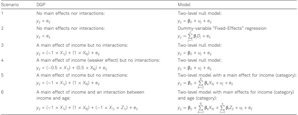
Table 1.Simulation scenarios
Scenario DGP Model
1 No main effects nor interactions: Two-level null model:
yij=eij yij=β0+uj+eij
2 No main effects nor interactions: Dummy-variable“Fixed-Effects”regression
yij=eij yij¼
PJ j¼1
βjDjþeij
3 A main effect of income but no interactions: Two-level null model:
yij= ( 1X1j) + (1X6j) +eij yij=β0+uj+eij
4 A main effect of income (weaker effect) but no interactions: Two-level null model:
yij= ( 0.5X1j) + (0.5X6j) +eij yij=β0+uj+eij
5 A main effect of income but no interactions: Two-level model with a main effect for income (category):
yij= ( 1X1j) + (1X6j) +eij yij¼β0þP
6
k¼2
βkXkjþujþeij
6 A main effect of income and an interaction between
income and age:
Two-level model with main effects for income (category) and age (category):
yij= ( 1X1j) + (1X6j) + ( 1X1jZ1j) +eij yij¼β0þP
6
k¼2
βkXkjþP
4
l¼2
βlZljþujþeij
Notes.Xkjis a dummy variable for income categoryk(k= 1,. . ., 6).Zljis a dummy variable representing for age categoryl(l= 1,. . ., 4);jrepresents intersections of income (6 categories), gender (2 categories), age (4 categories), and ethnicity (6 categories) making a total maximum of 6246 = 288 intersections. In each of the scenarios, residuals in the model are assumed to be Normally distributed, such thateijN0;σ2
e
, and (except Scenario 2)
ujN0;σ2
u
. In the DGPs,σ2
eis set to 1.
5We have not simulated systematically different sizes of intersections (
nj) in order to see the effect on shrinkage of the main effects/interactions,
without systematic differences innjinterfering with that.
interactions that should appear significant. In Scenarios1,2,
and5, this is simply the intersections that are deemed
statis-tically different from the average across the intersections. In Scenarios 3 and 4, we subtract the estimates from the
income-group average (example.g., the average residual estimate for strata in income category 1, the average in
income category 2, etc.) and test the significance of that
de-meaned residual, in order to find the value of the residual net of any main effects in the DGP. In Scenario6, we
sub-tract the income-age-group average (e.g., the average resid-ual estimate for strata in income category1and age category 1, etc.). We then use these to see the proportion of significant
results, averaged across the 100simulations. It should be
noted that Evans et al. (2018) do not suggest using these
the models used in Scenarios3and4to test specific
interac-tions; however we test these models because (a) others have suggested using such models in this way (Hernández-Yumar et al.,2018; Jones et al.,2016), and (b) the problems with
those models are indicative of the problems encountered with the main-effects model as well in Scenario6.
Residuals are also visualized with“caterpillar”plots from a single example simulation run (Rasbash, Steele, Browne, & Goldstein,2009, chapter3). We focus on statistical
sig-nificance because (a) it gives a clear way of quantifying the“wrongness”of the model (that is more difficult to do with size of the estimated residuals) and (b) it is the best way of testing how well the method compensates for multiple comparisons, where the interest is in statistical significance or lack thereof. The size of residuals is, of course also important (perhaps more so) when interpreting the meaning of the effects, and this is visualized in the caterpillar plots that we produce.
Results
The results are summarized in Table2and Figure1.
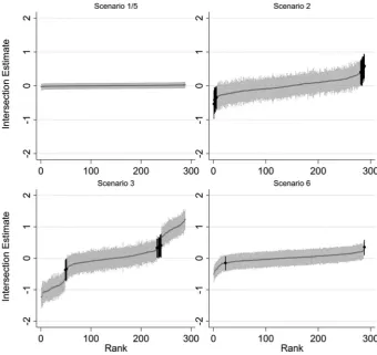
First it can be seen that, when there are no effects (either main effects or interactions) of the intersecting variables, multilevel models work well–no intersections appear signif-icant (Scenario1). This is an improvement on using
dummy-variable regression (Scenario2), where, as expected, around 5% of intersections are found to be statistically significant
despite no such effects existing in the DGP.
When there are main effects (Scenarios3and4), we see
that this “null” model performs less well, with between
0.1% and4% of intersections appearing statistically
signif-icant when there are, in fact, no such effects in the DGP. It is clear from this (and particularly clear in Figure1) that
there is less shrinkage in these scenarios than in Scenario1,
and this can be explained by the higher level-2variance that
is really the result of the main effects in the DGP. But that shrinkage is not only reduced in the intersections affected
by the main effect– it occurs in all intersections equally, meaning that there is more chance of finding significant effects when those effects are absent. There are some dif-ferences as a result of both sample size and effect size, but these do not seem to follow a clear pattern (other than that there is more shrinkage when the sample size is very small, which is to be expected given Equation4. Note that
the residuals successfully pick up the differences between groups that they are supposed to (see Figure 1, Scenario 3, where there are two clear groups of estimates appearing
different from the rest) but they also pick up other aberrant effects. It should be noted, though, that the fixed-effects/ dummy-variable approach will produce more unwanted effects, so this approach is still preferable to that.
In Scenario5, main effects were included in the model.
In this case, because these soak up all the main effects in the DGP, the remaining level-2 residuals will be as in
Scenario1. The result is a large degree of shrinkage, and
so no intersections appear statistically significant. However, this is not an all-purpose solution, since it only works if there are no additional interactions of the intersecting variables in the DGP. If there are such interactions (as in Scenario 6), these have a similar (though smaller) effect
as the main effects in Scenarios 3 and 4: increasing the
between-intersection variance, reducing the shrinkage, and increasing the chance of finding intersection effects where none exist. The effect is smaller than with main effects because fewer intersections are affected by the interaction, meaning the resulting level-2variance is
smal-ler. And, again, the model still outperforms the fixed-effects approach, where we would expect5% of the intersections
to appear significant just by chance.
Discussion
These simulations help us to understand when this model is valuable, and what its limits are. As stated above, there are two ways these models can be used: (1) to see whether
mul-tiplicative intersectionality matters generally, via the level-2
variance and associated VPC, and (2) to look at the level-2
residuals themselves. We argue here that the former is not problematic –the variance is in effect calculated prior to shrinkage anyway with most standard multilevel modeling estimation procedures, so is unaffected by any shrinkage that may or may not occur. From a policy perspective, the latter is often more interesting, but is found here to be more problematic–while it is an improvement on standard fixed effects dummy-variable regression, the amount of shrink-age is not always correct unless all true variable effects, including interactions, are included in the fixed part of the model. The inclusion of main effects improves the situ-ation, but does not solve it: if there are interactions between
Ó2019 Hogrefe Publishing Distributed as a Hogrefe OpenMind article
under the license [CC BY 4.0 (http://creativecommons.org/licenses/by/4.0/)]
Methodology(2019),15(2), 88–96
A. Bell et al., Using Shrinkage in Multilevel Models to Understand Intersectionality 93
variables, these will produce variance that changes the amount of shrinkage experienced by the intersection residuals.
One option could be an iterative approach, starting with a null model, then including first main effects (potentially one-by-one as suggested by Merlo, 2018), then two-way
(first-order) interactions, then three-way (second-order)
interactions, and so on until all the level-2 variance is
accounted for. Once these effects are in the fixed part of the model, there is less likelihood that the remaining inter-sections are the result of random chance. So long as at each stage all possible effects are included, this will not treat any particular variables as having primacy over the others (although, of course, it might find that a particular variable
Figure 1.Caterpillar plots showing example intersection effect estimates from a single simulation for four sce-narios (all using sample size of 10,000).
Intersections found to be incorrectly
[image:8.595.55.396.287.608.2]statistically significant are highlighted.
Table 2.The average proportion of intersections appearing incorrectly statistically significant (p< .05), for each scenario and with different sample
sizes (averaged across 100 simulation iterations)
Sample 1k (mean 3.6 obs/ intersection)
Sample 10k (mean 34.7/ intersection)
Sample 100k (mean 347/ intersection)
Scenario Mean Range Mean Range Mean Range
1 0 (0,0) 0 (0,0) 0 (0,0)
2 0.052 (0.022,0.117) 0.049 (0.021,0.087) 0.050 (0.024,0.799)
3 0.012 (0.000,0.052) 0.036 (0.014,0.068) 0.021 (0.0055,0.40)
4 0.001 (0.000,0.010) 0.022 (0.004, 0.049) 0.038 (0.011,0.068)
5 0 (0,0) 0 (0,0) 0 (0,0)
6 0.00005 (0,0.005) 0.004 (0,0.0183) 0.018 (0.003,0.036)
Notes. Scenario 1 has no effects in the DGP, and no main effects (only intersection random effects) specified in the model. Scenario 2 has no effects in the DGP, and the model is specified with fixed effect dummy variables for intersections. Scenarios 3 and 4 have no effects specified in the model, but large (Sc2) and small (Sc3) effects in the DGP. Scenario 5 has a large additive effect in the DGP, and additive effects (and random effects) specified in the model. Finally, Scenario 6 has large additive effects and an interaction effect in the DGP, with only additive effects (and the random effects) specified in the model. For Scenarios 3, 4, and 6, the fixed effects in the DGP that are not in the fixed part of the estimated model are subtracted from the residuals, so these do not include the differences we would expect given the real differences in the DGP.
or interaction is of particular importance in its effects). It should be noted, though, that effects in the fixed part of the model are not subject to shrinkage, so will become more at risk of multiple testing issues as multiway interac-tions increase. If we include final-order interacinterac-tions in the model, these will have the same issue of multiple testing as in the “fixed effects” approach with dummy variables outlined above. The advantage of this iterative approach is that we might not get to that point, if the level-2variance
reaches zero (statistically, based on model comparison statistics such as the Deviance Information Criterion, DIC, Spiegelhalter, Best, Carlin, & van der Linde, 2002)
as a result of the inclusion of lower order interactions. Indeed, this seems to be what happens for Johnston et al. (2018), who see the level-2 variance reach zero with just
the introduction of some two-way interactions. Similarly, if the variance reaches zero with just the introduction of main effects, that suggests there are no multiplicative effects (no interactions) at all. Once this has happened, one should not continue to test for higher order interac-tions, as significant effects are likely to be a result of multi-ple testing. If there remains variance at level2when all but
the final-order interactions are included, these would repre-sent the remaining, final order intersectional effects, net of lower order interactions, and are probably a better measure of their magnitude than fixed effects estimates (given, by this stage, most residual patterning should be removed to the fixed part of the model by the interactions).
A method like this could then be used to understand the extent and type of intersectionality experienced in the model, and how intersected the variables are. This is an extension of the method suggested by Evans et al. (2018)
–they compared the VPC of a model with no effects, and again with main effects, though they did not consider whether the remaining variance is the result of two-way interactions or more-way interactions. By seeing how the level-2variance decreases as increasing orders of
interac-tions are included, it would be possible to see how“deep” the intersectionality goes –whether it is the result of two variables interacting, three, or more.
Fisk et al. (2018), in their study of Chronic Obstructive
Pulmonary Disease, found that the level-2variance in their
logistic model reduced from an ICC of20% to1% with the
introduction of main effects in the fixed part of the model, finding only three significant intersections (out of96). They
downplay the importance of that 1% variance, stating the
three interactions are “about what would be expected by chance”(p.16). We disagree slightly with this interpretation.
First, our simulations suggest that intersections will be erroneously significant much less than5% of the time, given
at least some shrinkage will have occurred, so it is likely that those three intersectional effects are real. Second, in a logistic model, an ICC of0.01is a small but not substantively
insignificant effect size6
(Duncan & Raudenbush, 1999,
p.33), so the results imply that there remains some
poten-tially important intersectional effects. It would have been interesting to see (a) whether the remaining level-2variance
was statistically significant (compared via the DIC to a model without this term), and (b) whether the inclusion of two-way interactions reduces the variance, and significance of those three intersections. This would help to judge whether the remaining significant intersections were actually the result of low-order (e.g., two-way) interactions. Overall, these results can be summarized as“OK, but”. The model is an improvement on the dummy-variable fixed-effects approach, but it is not perfect, and the nuanced approach suggested above could improve it further. It is worth noting, though, that the approach is inherently exploratory and so will be most valuable when repeated studies show the same results.
It should be noted that the results found here have impli-cations beyond the study of intersectionality–it is relevant to all studies using multilevel models to identify“ signifi-cant”level-2units. For example, if a study of student
attain-ment finds that certain schools are significantly better or worse than others, it could be that there is an unmeasured attribute of the school that is causing greater level-2
vari-ance, reducing shrinkage and so introducing differences between schools that do not actually exist. This study should act as a warning (a) to include higher level variables as fixed effects in a multilevel model, and not to rely on higher level residuals to identify such differences, and (b) to not over-interpret differences between higher level units like schools, as in the presence of important unmeasured variables, they could be vulnerable to the perils of multiple testing.
References
Bauer, G. R. (2014). Incorporating intersectionality theory into population health research methodology: Challenges and the
potential to advance health equity.Social Science & Medicine,
110, 10–17. https://doi.org/10.1016/j.socscimed.2014.03.022
Bell, A., Fairbrother, M., & Jones, K. (2019). Fixed and random
effects models: making an informed choice.Quality & Quantity,
53, 1051–1074. https://doi.org/10.1007/s11135-018-0802-x
Bell, A., & Jones, K. (2015). Explaining fixed effects: Random effects modelling of time-series cross-sectional and panel
data. Political Science Research and Methods, 3, 133–153.
https://doi.org/10.1017/psrm.2014.7
Browne, W. J. (2009). MCMC estimation in MLwiN Version 2.25.
Bristol, UK: Centre for Multilevel Modelling, University of Bristol.
6An ICC of 1% in a logistic model is equivalent to a Median Odds Ratio (Larsen & Merlo, 2005, pp. 82
–83) of around 1.2, that is, the difference
between two intersections chosen at random is, on average, equivalent to a 20% increase in the odds ofY.
Ó2019 Hogrefe Publishing Distributed as a Hogrefe OpenMind article
under the license [CC BY 4.0 (http://creativecommons.org/licenses/by/4.0/)]
Methodology(2019),15(2), 88–96
A. Bell et al., Using Shrinkage in Multilevel Models to Understand Intersectionality 95
Charlton, C., Rasbash, J., Browne, W. J., Healy, M., & Cameron, B.
(2013).MLwiN version 2.28. Bristol, UK: Centre for Multilevel
Modelling, University of Bristol.
Choo, H. Y., & Ferree, M. M. (2010). Practicing intersectionality in sociological research: A critical analysis of inclusions,
interac-tions, and institutions in the study of inequalities.Sociological
Theory, 28, 129–149. https://doi.org/10.1111/j.1467-9558.2010. 01370.x
Crenshaw, K. (1991). Mapping the margins: Intersectionality,
identity politics, and violence against women of color.Stanford
Law Review, 43, 1241–1299. https://doi.org/10.2307/1229039 Duncan, G., & Raudenbush, S. (1999). Assessing the effects
of context in studies of child and youth development.
Educational Psychologist, 34, 29–41. https://doi.org/10.1207/ s15326985ep3401_3
Evans, C. R., Williams, D. R., Onnela, J. P., & Subramanian, S. V. (2018). A multilevel approach to modeling health inequalities at
the intersection of multiple social identities.Social Science &
Medicine, 203, 64–73. https://doi.org/10.1016/j.socscimed. 2017.11.011
Fisk, S. A., Mulinari, S., Wemrell, M., Leckie, G., Perez Vicente, R., & Merlo, J. (2018). Chronic obstructive pulmonary disease in Sweden: An intersectional multilevel analysis of individual
heterogeneity and discriminatory accuracy.SSM–Population
Health, 4, 334–346. https://doi.org/10.1016/j.ssmph.2018. 03.005
Green, M. A., Evans, C. R., & Subramanian, S. V. (2017). Can intersectionality theory enrich population health research?
Social Science & Medicine, 178, 214–216. https://doi.org/ 10.1016/j.socscimed.2017.02.029
Hernández-Yumar, A., Wemrell, M., Abásolo Alessón, I., López-Valcárcel, B. G., Leckie, G., & Merlo, J. (2018). Socioeconomic differences in body mass index in Spain: An intersectional multilevel analysis of individual heterogeneity and
discrimina-tory accuracy.PLoS One, 13, e020862. http://doi.org/10.1371/
journal.pone.0208624
Hill Collins, P. (2008). Black feminist thought: Knowledge,
con-sciousness, and the politics of empowerment. New York, NY: Routledge.
Johnston, R., Jones, K., & Manley, D. (2018). Age, sex, qualifica-tions and voting at recent English general elecqualifica-tions: an
alternative exploratory approach.Electoral Studies, 51, 24–37.
https://doi.org/10.1016/j.electstud.2017.11.006
Jones, K., & Bullen, N. (1994). Contextual models of urban house
prices – a comparison of fixed-coefficient and
random-coefficient models developed by expansion.Economic
Geogra-phy, 70, 252–272. https://doi.org/10.2307/143993
Jones, K., Johnston, R., & Manley, D. (2016). Uncovering interac-tions in multivariate contingency tables: A multi-level modelling
exploratory approach. Methodological Innovations, 9, 1–17.
https://doi.org/10.1177/2059799116672874
Larsen, K., & Merlo, J. (2005). Appropriate assessment of neigh-borhood effects on individual health: integrating random and
fixed effects in multilevel logistic regression.American Journal of
Epidemiology, 161, 81–88. https://doi.org/10.1093/aje/kwi017 Leckie, G., & Charlton, C. (2013). runmlwin: A program to run the
MLwiN multilevel modelling software from within Stata.Journal
of Statistical Software, 52, 1–40. https://doi.org/10.18637/jss. v052.i11
Marshall, S. W. (2007). Power for tests of interaction: effect of
raising the Type I error rate. Epidemiologic Perspectives &
Innovations, 4. https://doi.org/10.1186/1742-5573-4-4
McCall, L. (2005). The complexity of intersectionality.Signs, 30,
1771–1800. https://doi.org/10.1086/426800
Merlo, J. (2018). Multilevel analysis of individual heterogeneity and discriminatory accuracy (MAIHDA) within an intersectional
framework. Social Science & Medicine, 203, 74–80. https://
doi.org/10.1016/j.socscimed.2017.12.026
Pillinger, R. (2008).Residuals. Retrieved from http://www.bristol.
ac.uk/cmm/learning/videos/residuals.html
Rasbash, J., Steele, F., Browne, W. J., & Goldstein, H. (2009).A
user’s guide to MLwiN, version 2.10. Bristol, UK: Centre for Multilevel Modelling, University of Bristol.
Spiegelhalter, D. J., Best, N. G., Carlin, B. R., & van der Linde, A.
(2002). Bayesian measures of model complexity and fit.Journal
of the Royal Statistical Society Series B–Statistical Method-ology, 64, 583–616. https://doi.org/10.1111/1467-9868.00353 Yuval-Davis, N. (2006). Intersectionality and feminist politics.
European Journal of Women’s Studies, 13, 193–209.
History
Received April 4, 2018
Revision received December 13, 2018 Accepted January 23, 2019
Published online May 27, 2019
Acknowledgments
This work was supported by the Economic and Social Research Council [grant number ES/R00921X/1].
Andrew Bell
Sheffield Methods Institute University of Sheffield 219 Portobello Sheffield, S1 4DP UK