MoL 2007 03: Transfer Learning Using the Minimum Description Length Principle with a Decision Tree Application

Transfer Learning Using the Minimum Description

Length Principle with a Decision Tree Application

MSc Thesis

(

_{Afstudeerscriptie}

)

written by Höskuldur Hlynsson

(born May 27th, 1977 in Reykjavik, Iceland)

under the supervision of Dr Maarten van Someren, and submitted to the Board of Examiners in partial fulfillment of the requirements for the degree of

MSc in Logic

at theUniversiteit van Amsterdam.

Date of the public defense: Members of the Thesis Committee: April 4, 2007 Prof Dr Pieter Adriaans

Contents

Contents i

1 Introduction 1

1.1 Orientation and Outline . . . 1

1.2 Preliminaries and Notation . . . 4

1.3 Minimum Description Length Inference . . . 7

2 Transfer learning 12 2.1 Transfer learning . . . 13

2.2 A Communication Framework for Transfer Learning . . . 16

2.3 A Meta-Algorithm . . . 18

2.4 Discussion . . . 21

3 Convergence 24 3.1 Convergence Concepts . . . 25

3.2 Proof of Convergence . . . 26

4 Instantiation Of Meta-Algorithm 34 4.1 Decision Tree Learning . . . 34

4.1.1 General Ideas . . . 34

4.1.2 C45 and Weka’s J48 . . . 35

4.1.3 Obtaining Measures from Trees . . . 37

4.2 Coding Trees and Data . . . 38

4.2.1 Coding Trees . . . 38

4.2.2 Coding strings of ’0’ and ’1’s . . . 41

4.3 Instantiation of Meta-Algorithm . . . 42

4.4 How to Combine Environment Knowledge and Task Specifics . . 42

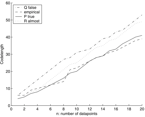
5 Experiments 45 5.1 Simple Simulated Example . . . 45

5.2 Decision Trees and Real World Data . . . 49

5.2.1 Implementation . . . 49

5.2.2 Data and Pre-Processing . . . 50

5.2.3 Experimental Results . . . 52

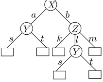
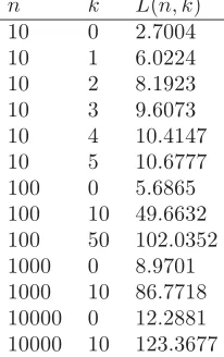
Appendices 67 A.1 Experimental Result Tables . . . 67 A.2 Relation between tree depth and codelength . . . 76

“ The Tarot has an unprecise relationship with the dimension of time. Contrary to popular opinion the cards cannot be used to predict the future. If the future were a definite and unalterable fact then the cards could be used to predict it. But the future is not a predetermined and planned event; if it were it would require a planner ([...] If the future were predetermined, then every detail of every event would have to be considered in advance, in effect creating the future in all its minutiae before it actually happens). What will happen tomorrow varies, sometimes subtly, sometimes dramatically. It is constantly adapting and changing, responding to the events and decisions made today. Viewed in this way, the future is not a definite and unavoidable fact; what actually occurs is one of a number of possibilities. The concept may be represented visually in the shape of a cone[...]. ”

— The Ancient Egyptian Tarot, by Clive Barret.

“ Prediction is very difficult, especially if it is about the future. ” — Attributed to Niels Bohr, Physicist.

“Predicting the future is as difficult as reconstructing the past. ”

Abstract

Chapter 1

Introduction

“ ’Begin at the beginning’, the King said, gravely, ’and go till you come to the end; then stop.” ’

— Lewis Carol, Alice in Wonderland

In this chapter we introduce the topic and the purpose of this paper and define the basic concepts and notation.

1.1

Orientation and Outline

This paper is about an approach to a form of meta-learning, ortransfer learning, as applied to supervised learning. Meta-learning studies how learning algorithms can increase their classification performance, as measured by e.g. error rate, through knowledge about previous applications. The difference between meta-learning and base-learning is in the way the algorithms obtain a bias on the learning procedure: base-learners have a fixed bias while the meta-learner tries to induce a proper bias for the specific learning task at hand, based on knowledge about previously analysed tasks. An example of a fixed bias is “Small decision trees are more probable than big decision trees”. An example of variable bias would be “decision trees from this task-determined collection of trees are more probable then others”. Base-learners seek to improve the quality of their learning as the number of training examples in a task increases; meta-learners seek to improve the quality of the learning-strategy as the number of tasks increases also. We can view meta-learning as ’learning from experience’ where experience is understood as knowledge obtained from analysis of several tasks. A survey of meta-learning is given in [VD02].

The specific instance of meta-learning we will address in this paper is how we transfer learning done over some collection of related tasks to a new task where information about the datasets from the old tasks is withheld and only the learned structures are available. To motivate our approach, we allude shortly to our framework. First, we’ll give a couple of examples of what sort of problems we have in mind.

condi-tion affecting an organ. Each hospital only has informacondi-tion about the measure-ments it makes on its own patients. Other hospitals have made the same sort of tests but because of privacy legislation cannot share their data. There are no limitations on sharing knowledge not traceable to individuals, which they do by making summarized information available in the form of learned structures. Now, a clinic starts testing for this condition. How can it make its procedures more effective by using experience gained on its own patients and the knowledge about others experience?

Example Language acquisition A person knows Portuguese and Italian and is learning Spanish. How can knowledge of the other two languages be of use? That person can both benefit from associating grammatical rules (syntactics) and word structures (semantics) from the languages already studied to the new one, without referring to specific examples (words/sentences).

We formulate our approach to transfer learning as a communication problem and use the Minimum Description Length (MDL) principle as the induction principle. When we speak ofknowledge we mean a hypothesis which will almost always be uncertain, i.e. only true to a degree in relation to a dataset.

Consider the following scenario: I have some knowledge constructed from a particular collection of related application domains1_{, which we term an} envi-ronment, and you have a dataset, perhaps a small one. You decide that your learning task is in some way similar to the domains that I have knowledge of. You therefore acquire the knowledge that I have but not the data. Based on your data you decide what knowledge is applicable to your learning task, if any. I can not show you my data, from which I learned. Whether we share which learning algorithms were used is of no significance.

Furthermore, my knowledge must in some way simplify, or accelerate, your learning task in the sense that the probability of error decreases. Otherwise it is of no practical use to you. We like things to be as simple as possible, so you will not adopt overly complex knowledge to describe your data. There are two reasons to prefer simple explanations, all other things being equal: they are easier to remember and have less risk of explaining noise.2 _{However, you} might like the knowledge you adopt to be slightly more complex then what you would induce from your dataset alone. Otherwise you would just describe the knowledge you can draw from your dataset in form of a hypothesis without my assistance.

There must be some sort of a balance between the knowledge you adopt from my collection and how well this knowledge describes your data. When you adopt knowledge from my environment based on your limited data, you have transferred knowledge to your learning task. In order to give the knowledge which can be derived from your own dataset alone some part in our inference procedure, you add that knowledge to the environment3. After all, you are

1_{In what follows, the term}

domain refers to something abstract and conceptual which is assigned meaning by people. Domains do not have instantiations; example spaces, which are defined later, do have instantiations in the forms of datasets or samples.

2_{Some disciplines are more prone to explaining noise then others: the financial press is}

perhaps the most eager to offer explanations for everything. In general, every change (or lack there of) has an explanation. Elaborate explanations of minute price movements (less then 1/1000 of a percent) abound.

3_{This may appear strange, but there are strong theoretical reasons for doing this, as will}

hypothesizing that your dataset belongs to the environment. A formalization and an exploration of a framework for inducing transfer along these lines is the subject of this paper.

Why is transfer learning useful? Transfer learning is of use since we almost never have enough data. Enough data would be so much data, that more data would not give us any information that would be of practical use. This is a com-mon problem of inference. For instance, in [BC91] they talk aboutn= 1000000 to get a estimate of variance correct to 10bits4_{from a normal distribution. By} including information about the environment from which the data originates, we would hope to make up for the lack of data and obtain better hypothesis, as measured by error rate, while guarding against inapplicable information. An instance of this would be to obtain the same results with little data as with much data.

The learning task may thus be phrased as:

Given a learner, a collection of hypotheses derived from related data-generating domains and a dataset for a new task (hypothesized be-ing) related to the given collection, find an optimal hypothesis de-scribing the domain of the given dataset, such that it maximizes performance on the new task.

We will elaborate on the terms used in the statement of the task to give it more precise meaning as this paper develops. The important part is that the data we are given is supposed to be of a similar kind as the domains giving rise to the knowledge. We use parallels and similarities when solving tasks in our daily lives. Doors to cars open in a very similar way to those of houses, although car doors never open into the car, this is very common for doors to houses to do. The omission of the data giving rise to the knowledge may seem restrictive, but in a way emulates how humans operate. We’ve openeda lot of different doors in our time and learned that there are basically only a few things to keep in mind: first turn, twist or yank, then push or pull. When faced with a new door we will not recall all those doors we’ve opened, just the main principles. If the door is to a house and has a handle, try turning the handle, then push. When successful, we have learned how to open yet another door. We frequently make do with abstractions.

The development of the framework encapsulating this sort of inference pro-cess described above will be based on minimizing the communication cost of the knowledge used to describe the new data and the new data with respect to that knowledge. The rationale for this sort of inference will be given in Section 1.3 on MDL.

In order to give expressions about the scenario described above precise mean-ing we will need definitions from measure and learnmean-ing theory which are intro-duced in the next section. Then, after discussing the MDL principle for predic-tion and learning, we can give a definipredic-tion oftransfer and give a meta-algorithm for transfer learning. We are interested in asymptotic properties of the meta-algorithm and we give a proof of convergence in the chapter thereafter. To show how this framework might be put to work, we give an instantiation of the meta-algorithm using decision trees and give examples of its use in the final chapter.

1.2

Preliminaries and Notation

We are liberal in notation and will usexato mean concatenation of the symbols

xanda. A little more formally,xa∈X×A, where typicallyXis some cartesian product of the set A; Ais frequently referred to as an alphabet. For instance,

ifx= 10011∈B5 _{anda= 0∈B, then xa= 100110∈B}6_{. whereB={0,1}.}

We define a measure:

Definition 1.2.1 Let Ω be a set and F ⊂ P(Ω), where P(Ω) is the set of all subsets of Ω. A measure is a function μ : F → [0,∞[ such that for any enumerated sequence{E_i}of disjoint sets fromF we have countable additivity:

μ(∪∞_i=1Ei) = ∞

i=1

μ(Ei)

A probability measure is a measure taking values in [0,1], such that μ(∅) = 0

andμ(Ω) = 1.

We have the usual definition of conditioning on measures:

μ(y|x) = μ(xy)

μ(x) .

Two functions, or random variables, x, y : X → R, X an object space, are independent with respect to a measureμiffμ(xy) =μ(x)μ(y).

We will refer to a anti-semi measure property of some estimators and pre-dictors:

Definition 1.2.2 A semi measure is a function μ : Ω∗ → [0,1], such that

μ(∅)≤1 andμ(x)≥_a∈Ωμ(xa).

Semi measures thus allow for ’probability leaks’.5 _{Theanti-semi measure} prop-erty corresponds to the last inequality in the definition reversed. When dealing with binary classification problems the set Ωis{0,1}.

When we talk about probability measures we always have a σ-algebra in mind:

Definition 1.2.3 A σ-algebra F on Ω is a collection of subsets of Ω which satisfies∅ ∈ F,

Closure under countable unions: ∀i∈I⊆N (si∈ F)−→

i∈I si∈ F and

Closure under complementation: s∈ F −→¯s∈ F,

where ¯s denotes the complement of the set s and N is the set of the natural numbers.

The space (Ω,F) is called measurable and (Ω,F, μ) is called a measure space, where μ is a measure onF.

5_{Semi measures arise naturally in Solomonoff’s universal induction, see [Sol64], and account}

We need to restrict our attention to some proper subset ofP(Ω)when talking about measures over subsets of the setΩ, since generally if we accept the axiom of choice and countable additivity there are non-measurable sets in P(Ω). A

σ-algebra is such a restriction which has the desirable properties for dealing with outcomes of trials. 6

We don’t need the full measure theoretic heavy machinery to obtain our results. We can make do with the following definition of an expectation:

Definition 1.2.4 The expectationof a function ϕ: Ω→R with respect to a measureμis, for all ω∈Ω,

E ϕ=E_μ ϕ(ω) =

ω∈Ω

ϕ(ω)μ(ω).

The subscriptμis left unspecified when there is no risk of confusion.

When we are learning from data, we need some input to learn from, and when we are learning under supervision we also have some class labels of the input data. Our data comes from anexample space, whichreality generates.

Definition 1.2.5 Reality7 _{generates the pairs (x}

1, y1),(x2, y2),(x3, y3), . . . of

examples. We call x_i an object andy_i a (class) label. The objects and labels are from measurable spaces X and Y named object space and label space, respectively8_{. We require X =∅ and an σ-algebra on Y different from {∅, Y}.} An example space9_{is thenZ=}

defX×Y.Asampleor datasetSnis a particular

set of observed values of Zn_.

This definition implies that there are no missing observations in our samples. The requirement on theσ-algebra overY is because, were it not satisfied, there is no learning to be done, since there is essentially just one label to choose from. An object consists offeatures orattributes. If|X|=nthen we havenfeatures, referred to by ξi,1, ξi,2, . . . , ξi,n for theith object.

A function μ : X → Y, which may have generated the data, is called a concept and is necessarily measurable10 _{If such a function doesn’t exist, there} is no learning to be done. We will only be interested in stochastic concepts, for which either the concept is noisy itself or the observation process is not exact.

In what follows all functions will be assumed to be measurable, unless oth-erwise stated.

Definition 1.2.6 Alearning algorithm, or a learner,Lis a functionL:Zn_→ HL, where HL is a set of available concepts for the algorithm to learn. Each h∈ H_L is a function fromX toY, from the objects to the labels. We callH_L a hypothesis space. A hypothesis space is completeif it contains the trueconcept that generated the data.

6_{We note that aσ-algebra corresponds to a set of computable inputs to a fixed universal}

Turing machine.

7_{We won’t attempt a definition of this thing and trust the readers intuition.}

8_{In what follows, we useXinstead ofΩabove and view random variables and their domains}

as essentially the same thing.

9_{Sometimes referred to asinput-outputspace.}

10_{If it were not measurable, it wouldn’t be computable and thus the concept not learnable.}

An instance of a learner is a classifier, i.e. given a sample Sn _{from Z}n _we

have L(Sn_{) =h, where h∈ H}

L, so a classifier is a function L(Sn) =hand is

applied to objects to be classified byL(Sn_{)(x) =h(x)∈Y.}

The subscript for the hypothesis space will be omitted when there is no ambiguity. If a space contains all functions from the input space to the output space, it is obviously complete.

When have a dataset from an example space and want to construct a classifier to classify previously unseen objects, we face a learning problem, or a task, in which we try to recover (learn) aconcept which presumably generated the data. Learning can be done in eitherrealizableornon-realizable setting, depending on whether thetrue hypothesis is available to the learner or not, respectively. The learner solves this learning problem and produces a classifier. The learner does this by searching through a space of functions available to the algorithm for a function that best fits the evidence of the dataset in some sense. This space is frequently unstructured and the search procedure is subject to converging to local optima. Thus we would like to influence the search for a good hypothesis by directing the search procedure in a certain way by inducing asearch bias on the learner.

Definition 1.2.7 A search bias on a learner is a partial ordering of H, i.e. ∀a, b, c∈ H the following hold: aa,ab∧ba→a=b andab∧b c→ac.

A bias of a learnerAis strongerthen that of B if |H_LA| ≤ |H_LB|.

The search bias is important, because we are often happy with methods that stop at local optima and which local optima we get stuck in during the search depends on the order. Later in this paper, we will use a description length function to impose the order on H. In another light, we would like to impose an ordering onH, s.t. we get a goodh∈ Hearly on in the search. An example of such a bias are those of decision tree construction algorithms which do not consider more complicated trees if they can make do with the simpler ones.

There are other types of bias concepts in use for learning theory: generally it refers to “any basis for choosing one generalization over another, other then strict consistency with the observed training instances” [Mit80]. The search bias is a relativebias, as it does not exclude hypotheses but orders them. Another type of bias is thestrict, which excludes hypotheses from the space under consideration. These are said to be strong or weak, depending on how aggressively they exclude hypotheses, as indicated in the last definition.

Another characterization of bias is theinductive bias, which is the minimal set of assertionsBsuch that for any conceptμto be learned and the sampleSfor the learning such that the classification of any objectx∈Xfollows deductively. That is

∀x∈X(B∧S∧x) L(S)(x)

This differs from the earlier concepts of bias in that it doesn’t operate directly on the hypotheses space.

There are various methodologies used to infer a function from some collection based on data. In the next section we describe the minimum description length principle (MDL), which is such a method. Another method related to the MDL is described in 4.1.2 on decision tree learning. The decision tree method also gives a nice way of representing the learned functions.

1.3

Minimum Description Length Inference

“ The fundamental idea behind the MDL Principle is that any regularity in a given set of data can be used to compress the data, i.e. to describe it using fewer symbols than needed to describe the data literally.”

— [Grü98]

“ We never want to make the false assumption that the observed data actually were generated by a distribution of some kind, say Gaussian, and then go on to analyze the consequences and make further deductions. Our deductions may be entertaining but quite irrelevant to the task at hand, namely, to learn useful properties from the data.”

— [Ris89]

When we want infer a mathematical description of some data generating process which captures its underlying structure, we are inferring a function. How we do that is based on the inference principle11 _{we adopt. Inference is} conceptually rather tricky. Consider the following example:

Example Given ’010101’ from{0,1}∗, a set of arbitrary length strings of ’0’ and ’1’, which pattern should we infer when given a choice between

1. Repeat ’01’ 2. Repeat ’010101’ 3. Repeat ’010’ ?

Which explains the data best? Which is the simplest? What if we are also given the strings ’01101’ and ’01010101’ as examples?

The function we are inferring, the “explanatory theory”, we call ahypothesis and group together in hypothesis spaces12, which are collections of hypotheses. When talking about models we usually have a specific restriction of the hy-pothesis space in mind, as may be expressed by a parametrization of a specific functional form such as the normal or beta-distribution.13_{We will use the term}

11_{An inference principle is essentially the same as a bias.}

12_{These are always required to be sets.}

classification model in the same way as hypothesis though and refer to param-eterized models when we are talking about such things. The termknowledgein this paper is also the same as hypothesis.

When inferring a hypothesis based on some data we need to state explicitly the principle we are using on each occasion. There are essentially two ways of dealing with this sort of scenario, each with its ancient advocate. The first is to ’not multiply explanations beyond necessity’ and is referred to as Occam’s razor and finds its modern embodiment in the MDL principle, which we adopt in this paper. The second is the Epicurean principle of multiple explanations: if more than one hypothesis is consistent with the observations, keep all of those. Epicurus’ principle relates to Bayesian mixture probabilities, which will be defined later, and prediction with expert advice, which will not be discussed at all in this paper, but see e.g. [Vov98] for a discussion of this very interesting approach.

The most intuitively appealing way of inferring a function which is to de-scribe some datasource from sampled data is the Bayesian approach. Although ideal, there are however considerable difficulties in specifying the prior prob-abilities necessary for applications. This problem can be circumvented to an extent by making the inference procedure as purely data-dependent as possible. The Minimum Description Length (MDL) style of inference take that approach and the strength of the inference procedures is almost as good as that of the Bayesian. Instead of probability we use description length, which is equivalent to probability as will be explained. For practical applications, MDL promises to be a good approximation. 14

Why should we base an inference procedure on a description length concept? This is motivated in a sender-receiver setting, where the sender has a dataset and a set of hypotheses to describe the data with. The sender wants to communicate the data as efficiently as possible to the receiver, and can use hypothesis to describe his data more compactly. Thus, he uses the hypothesis to compress the data and transmits the data by coding a model and the data w.r.t. the model using a suitable encoding, or description method. We define the MDL principle as follows:

Definition 1.3.1 Given a sample of data D and a countable collection of hy-potheses Hthe MDL principle is to select theH ∈ Hwhich minimizes the sum of

• the bit length of the description of the hypothesisH and

• the bit length of the description of the data based on the hypothesisH15_. The first term is abbreviated as LC1(H)the second LC2(D|H)so the principle

is to select the hypothesis HMDLsuch that

HMDL= arg min

H∈H

{LC1(H) +LC2(D|H)},

whereC1 is the description method for the hypothesis andC2 is the description

method describing the data w.r.t. the hypothesis.

14_{There are close similarities between the Bayesian method and MDL, but MDL deals}

with codelengths while Bayes with probabilities and there exist some differences between the inferences made. MDL has a existence separate from the Bayesian methodology. For more, see [Grü04].

We will not distinguish between the two description methods involved in the definition and assume that the difference is understood.

An interesting thing is that every induction problem can be phrased as a bi-nary sequence prediction problem and classification is a special case of sequence prediction. This is the power of the universal Turing machine.

The MDL principle tries to strike a balance between how complex the hy-pothesis is and how much it “explains” the data. The main motivation is to avoid overfitting the hypothesis to the data, i.e. modelling the noise. We want to factor out the regularities in the data by using our collection of hypotheses but leave the (suitably random) noise. This could be phrased as selecting an hypothesis that gives an optimal balance between how complex the hypothesis is and how well that hypothesis explains the data and thus an instance of Occam’s razor.

The MDL principle might seem a bit arbitrary. A justification of the prin-ciple based on Bayesian learning theory follows.

When learning from data we have some collection of hypotheses H about the data to choose from. Before observing any data we might claim some dis-tribution overH, given byP(H). After observing some data we hopefully gain some useful information about which hypotheses are more likely then others, obtainingP(H|D). An appealing way to select a hypothesis fromHis to select the most probable one after observing the data. This gives the maximum a posteriori (MAP) hypothesis:

HMAP = arg max

H∈H

{P(H|D)}

= arg max

H∈H

P(D|H)P(H)

P(D)

= arg max

H∈H {P(D|H)P(H)}

= arg min

H∈H {−log2P(D|H)−log2P(H)}

where we have dropped P(D) since it doesn’t depend on H. Observe that if eachH has the same probability we get the maximum likelihood estimator

HML= arg max

H∈H

P(D|H).

Now, to go from HMAP to the hypothesis selected by the MDL principle

we need to observe that codelengths are equivalent to probabilities. Thus, in a sense, we obtain the Bayesian priors via codelengths. This relation is given by a fundamental inequality from information theory, namely the Kraft inequality. First, we define what is meant by adescription method, and related concepts. Definition 1.3.2 Let A be an alphabet. A coding system C is a relation be-tween Aand∪_k≥1{0,1}k_{. If (a, b)∈C then we say that bis a codeword for a.}

A description method is a coding systemC such that for each b∈ ∪_k≥1{0,1}k

there is at most one a ∈ A with (a, b) ∈ C The description length of a ∈ A

under a description methodC is the cardinality ofb, such that(a, b)∈C.

whenever we talk of description methods, we are talking about prefix descrip-tion methods. For details about MLD, see [Grü04] , for the Kraft inequality giving the correspondence between prefix description lengths and probability distributions:

Theorem 1.3.3 For any prefix description method C for a finite alphabet A=

{1, . . . , m}, the codeword lengthsLC(1), . . . , LC(m)must satisfy

a∈A

2−LC(a)_≤1.

Conversely, given a set of codeword lengths satisfying the inequality, there exists a prefix description method with these lengths.

A proof may be found in [CT91], Section 5.2.

This tells us that there exists a (defective) probability distribution16

P(x) = 2−LC(x)_,∀x∈Ω.

17_{Of course, we choose the correspondence in such a way that short codelengths} correspond to high probability, and vice versa. With the correspondence be-tween codelengths and probabilities we get the MDL principle as it is stated above.

When using MDL for prediction there are three ways to proceed, all based on the idea of using the best model from the class. We give descriptions of these methods when we need to use them in Section 3.2

Much can be said about MDL and its relation to Kolmogorov complexity (KC) but this is sufficient for our purposes. See e.g. [LV97] and [Grü04] for more on KC and MDL.

Although a very powerful inference principle with solid theoretical and philo-sophical foundations, the MDL principle does have some shortcomings. Criti-cisms and a list of problems is for instance given in [HOGV04].

To conclude this chapter, we pick up the examples from Section 1.1 and see what the MDL principle has to say about them intuitively. In the next chapter we’ll give a definition of transferability based on MDL.

Example Language acquisitionConsider a collection of grammatical rules from Portuguese and Italian and a dataset consisting of sentences from Spanish, along with their part-of-speech tagging. Inferring which rules apply sufficiently well to justify using them to assist in acquiring Spanish can be done using MDL. We evaluate the usefulness of the given grammatical rules by applying them to the collection of sentences and seeing whether the sentences are described in a shorter way by the help of the rules then without them. That is, if we can compress the given corpus by using the rules. Or, in more common language, if it is easier to remember the sentences by the help of a rules, that rule is useful. As it happens, our brains seem to be wired especially well to deal with grammatical rules.

16_{Adefectiveprobability distribution fails to satisfy}

x∈ΩP(x) = 1,Ωan outcome space,

but satisfies_x∈ΩP(x)≤1.

17_{The Shannon-Fano codes have these codelengths. Moreover, in Solomonoff’s universal}

Chapter 2

Transfer learning

Transfer learning deals with using knowledge obtained from one learning task in another learning task. In general, transferring knowledge is difficult for us humans. Teachers report that children don’t apply knowledge they obtained in one subject to another until they have developed considerable cognitive abilities, see e.g. [Has00] for a cognitive perspective.

In recent years researchers have started to focus on algorithms to transfer learning and the momentum seems to be increasing. Prominent institutes such as The Defense Advanced Research Projects Agency (DARPA), an agency of the United States Department of Defense responsible for the development of new technology for use by the military, have started to funnel funds to research in that area. To quote the DARPA project description BAA05-29:

1.1 PROGRAM OBJECTIVES

The goal of the Transfer Learning Program solicited by this BAA is to develop, implement, demonstrate and evaluate theories, architec-tures, algorithms, methods, and techniques that enable computers to apply knowledge learned for a particular, original set of tasks to achieve superior performance on new, previously unseen tasks. This goal reflects the observation that key cognitive abilities of hu-mans include the abilities to generalize, abstract, reuse, reorganize and apply knowledge learned in previous life experiences to novel situations.

This agrees with our view that successful development of transfer learning theories are a fundamental stepping stone towards a truemachine intelligence. Machines capable of transfer learning would display cognitive abilities far beyond those seen so far. One might even venture so far as to say that when we have good transfer learning paradigms the development of machine learning will first take flight, perhaps on its own accord.

2.1

Transfer learning

When we acquire a dataset from some example space, we think of the data as arising from some domain that encapsulates some structure governing its behaviour. This term “domain” is necessarily somewhat vague and subject to interpretation. Two or more example spaces can be thought of as being related if their domains are related. Thisrelatedness concept is quantified with respect to some task by thetransferable notion defined in def. 2.1.2. 1

For instance, two medical diagnosis tests, i.e. classifiers, of diseases affecting the same organ may be thought of as related domains, since the organ has some structure governing the behaviour of the diagnosis. If we have one or more histories of diagnosis test for some organ, and are devising a new test then we would like to use the information already obtained about the structure of diseases affecting that organ to speed up the learning of the structure for the new test.2 _{In essence we would be transferring knowledge about the organ itself} since the diseases exploit weaknesses in organs. Thus, we would like to group the other tests into anenvironment and transfer the learning from the environment to the new application domain. We define an environment as follows:

Definition 2.1.1 An environmentE is defined byE= (∅, Z1, Z2, . . . , Zn),n∈ N, n >0, whereZi, i∈ {1,2, . . . , n}, are example spaces.

We include the empty set for technical reasons. Including it allows for a default behaviour of doing nothing.

1_{Another related point of view is provided by the hierarchical Bayes, which can be sketched}

as follows in its basic form. Given several sequences of random variablesx1, x2, . . . , xm, each with corresponding length of ni, i = 1, . . . , m, ni ∈ N, which are unrestrictedly infinitely exchangeable have a joint density

p(x1(n1), . . . , xm(nm)) =

Θm

m

i=1

ni

j=1

p(xij|θi)dQ(θ1, . . . , θm),

whereQ(θ1, . . . , θm)is the prior overΘm. In general, nothing can be said aboutQ. However, if thexis are such thatQhas interesting structure then various forms of hierarchical models arise. Thus, we quantify therelatedness of thexis through the structure ofQ. This leaves it up to the modeler to decide which forms ofQare interesting. This might be quantified by the Kullback-Leibler divergence between Qand a uniform distribution or a non-informative prior of the same dimension, for instance. One interpretation of the KL-divergence between two distributionsP andQis, that it is the expected number of extra bits needed to encode an event fromP if the code used corresponds to the distributionQ.

A generic density version of such a model might take the form:

p(x1, . . . , xk|θ1, . . . , θk) = k

i=1

p(xi|θi) (2.1)

p(θ1, . . . , θk|φ) =

k

i=1

p(θi|φ) (2.2)

p(φ) (2.3)

The difference between this model and ordinary learning is that the bias of the learner, eq. (2.2) is now conditioned on ahyper parameter φand this has ahyper biasas represented by the distribution in eq. (2.3).

This seems like a fruitful way to look at transfer; for the interpretation and further discus-sion, see [BS94]. To make the connection with our framework, we would need to limit the attention to sufficient statistics arising from the given sequences. This will not be further pursued in this paper.

Note that there is no mention of the example spaces being in any way related. We would however hope that the underlying domains would be related in some way, although it is difficult to quantify this3_{. Transfer should occur when there} is a computable relation between the domains. If there is no such relation, no transfer should occur. The understanding of an environment given above also permits a single non-empty domain to be used for transfer.

The primary goal of grouping example spaces into an environment is to draw useful knowledge from it for transfer to a new domain and its example space. This makes us wonder if we can require some of the features to be the same, in some sense. However, that sort of requirement would always be superficial at best. The features temperature and pressure occur in may domains4. We have no reason to suspect that measurements of temperature and pressure in a two different situations reflect knowledge from related domains. For instance, one set of measurements might come from a situation where we are deciding to play tennis. Another from a geological investigation of a geothermal drilling hole drilled for deciding if to harvest the energy. Simple syntax is of little use for grouping domains into environments; we need to consider why we are solving particular classification problem. There is art in the construction of useful environments.

We can however talk about knowledge contained in an environment without complications:

Definition 2.1.2 Given an environment E = (∅, Z1, Z2, . . . , Zn), n ∈ N, the

environment knowledge5_{is a collection of classifiers} ME = (h1, h2, . . . hm),

such that

∀i∃j(hj =L(Zi)), j∈ {1,2, . . . , m},

i.e. there is at least one instance of a learner for each classification source con-stituting the environment.

Say we have a new domain and an associated example space Z_k+1. We want to build a classifier for the new domain and have a datasetSn

k+1,n∈N.

We suspect that Zk+1 belongs to an environmentE = (∅, Z1, Z2, . . . , Zk). In

order to make use of the available information we need some measurement of “transferability”. Also, as the datasetSn

k+1 grows6, we would presumably like

to adopt more detailed or complex knowledge from the environment since our confidence in the environment knowledge grows. Thus, we would like knowledge of different complexity to choose from. We can induce knowledge of different complexity from the environment knowledge by restricting attention to a subset of the features available from each domain or a subset of the values that each

3_{This issue refers to themeta-meta-natureof the problem, similar to the way that transfer} learning refers to the meta-nature of the original learners.

4_{These have a well defined meaning in physics and obey the equation of state for an ideal}

gas: P V = N kT, where P is pressure, V is volume, N is the number of molecules, kis Boltzmann’s constant andT is temperature. In a classification setting objects get another less quantifiable dimension: thepurposeor goal of the task.

5_{The word “knowledge” is used to refer to uncertain, i.e. statistical, knowledge too.}

6_{In the real world, we are frequently faced with a situation where more data becomes}

feature can take. A formal definition of this sort of restrictions is technically not straightforward and will not be attempted here. Selecting the features for inclusion in a restriction of specific size is the feature subset selection problem, which has been studied extensively.

A sensible way to partition the knowledge for use from each domain is to take the most informative set of features, w.r.t. the dataset from that domain, from each domain in increasing order of conditional complexity of the resulting classifier, given the features already selected. So, we first select the single most informative feature, then the two most informative features, the second condi-tional on the first, and so forth. Thus we get the best quality of hypothesis for each complexity, as measured by the hypothesis codelength, and a linear order-ing of these optimal hypotheses with respect to the total codelength. These we then evaluate with respect to data to choose a suitably sized hypothesis.

As an example, for decision trees constructed by an information theoretical measure such asinformation gain, , defined in 4.1.2, this procedure takes place quite naturally. There is no need for the learner to evaluate the informativeness of restrictions of different sizes w.r.t. a dataset, as that information is encoded into the tree when it is constructed.

An information measure quantifies the amount of regularity that a function distills from a dataset, loosely speaking. Examples of such an information mea-sure is information gain and the MDL codelength function. Our primary tool for evaluating the usefulness of an environment is that of transferability which we define in terms of a modified minimum description length principle. We introduce weights over the environment knowledgeM_E to reflect that we have more information then just the data alone. This information may be subjective. The weights are functions from the environment knowledge to the positive reals. These are discussed further in Sections 2.3 and 2.4.

Definition 2.1.3 Given environment knowledge ME and weightsw(h) we say that the knowledge contained in h ∈ M_E is transferable with respect to the datasetSn

k+1, n∈N, if

Lwh_C (S_kn₊₁) =_def L_C(S_kn₊₁|h) +w(h)L_C(h)≤L_C(S_kn₊₁).

The collection of all transferable classifiers we call the transferable set

Note thatLC(∅) = 0and we always have the empty set inME so the transferable

set contains ∅ at least. When selecting between two hypothesis of the same complexity, we would of course consider the one which is more informative. This is relevant for both construction of new hypotheses in ME and selection of hypothesis for transfer.

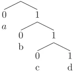
When coding the data with respect to the empty hypothesis for a binary classification problem, we will use one bit to designate the default class and then code the exceptions from that class. This corresponds to a very naïve Bayesian classifier which just uses the most frequent class as its prediction. The encoder the codes the exceptions from this class. We give more detail on this sort of scheme in Section 4.2.2.

Note also thatLwh

C (Skt+1)defines a linear order on any collection of

not size. In most applications we have approximate codelengths but not optimal ones.

Now we can answer the question: How do we select knowledge to be trans-ferred?

Transferh∗, s.t. h∗= arg min

h∈ME

Lwh_C (S_kn₊₁).

Before giving a statement of the proposed algorithm, we motivate it further in a communication framework.

2.2

A Communication Framework for Transfer

Learning

In this section we will show how to extend the basic sender-receiver setting underlying the minimum description length principle to cover the present setting in line with our definition of transferability. We also illustrate the relation between the algorithms involved in our framework.

We consider it our goal to perform well on the new task, for which we have data, using the knowledge available from the environment as well as we can. This may involve assigning different weights to the available hypotheses, depending on how credible we think they are. For instance, hypothesis occurring in many domains might be considered as more probable then others. We are minimizing the communication cost of the new dataset to a receiver, which we use the prior information to help us to do. We are not too concerned with time or memory complexity; the only thing we require at this stage is computability.

Now, recall the discussion from Section 1.1. We are now ready to make things a bit more precise, by using definitions given so far. When thinking about transfer learning in terms of a communication framework we need to state who communicates what to whom. Our problem is then to utilize the communication channelsas efficiently as possible. We do that by encoding our data as efficiently as possible. To begin with, we’ll assume that all learners involved are using the same learning algorithm. We’ll discuss how this assumption can be relaxed at the end of this section.

If you like a hypothesis from the collection of hypotheses that I give you, you may feel like combining more then one hypothesis into a more elaborate one.

The foregoing discussion raises a few questions for you:

• What are those theories or hypotheses?

• How do I decide that a hypothesis describes my data well?

• How do I describe a hypothesis?

• How do I describe my data w.r.t. a hypothesis?

• How can I gain confidence using that the knowledge I am adopting will actually help me to learn the structure of the new learning task?

• Will I be adopting different theories from your environment, coming from different domains, as my dataset grows?

• How can I gain more certainty in that any of your theories apply to my domain?

The first two of these questions are the main concerns of this paper. The theories to be considered are those that come from a learner which has been applied to an environment. The theories that describe the data well are the transferable hypotheses. The answers to the remaining questions are given by our MDL inference principle.

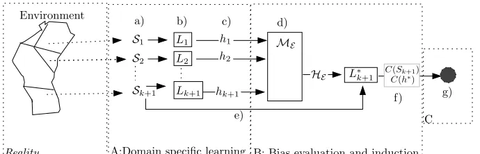
For ease of discussion, lets say that I, call me A, have the knowledge from an environment expressed as hypotheses from a learner. You, called B, have a small dataset from a new domain, and you are communicating your data to a third party, called C. The party C only plays a conceptual role in our scenario. You and C share the feature data (the input objects) of the dataset, but C doesn’t know the classes that each object belongs to. Thus, you only have to communicate the class-labels to C. If the structure of B’s learning problem is less rich then A has to communicate, B just ignores what is irrelevant. This scenario is illustrated in Figure 2.1

L₁

S1 M_E

f) b) c) d)

L2 S2

Lk+1 Sk+1

e) a)

A:Domain specific learning B: Bias evaluation and induction C Environment

g) h1

h₂

h_k+1

Reality

HE L∗k+1 C(h∗)

C(Sk+1)

Figure 2.1: The communication scenario for transfer learning The agents A, B and C communicate the knowledge and data as shown

a) Data Our data comes in the form of a sample from some datasource, which presumably hassome structure, S_k+1 is included, as per the assumption. b) Learner The learners do their thing with the data, including Lk+1. In

general, we need only restrict the learners such that they have the same representation of the learned hypothesis.

c) Each learner sends the learned hypothesis toM_E.

d) M_E: B is allowed to add hypotheses to M_E, by deriving new hypothesis from the given ones. In an adjusted measure of the applicability of the hypothesis, each hypothesis is given weight according to their origin and frequency, i.e. whether they come from the environment or induced from theSk+1 dataset. HE is thus the set of hypothesis proposed by the

envi-ronment, consideringSk+1as a part of it.

HE represents the knowledge available to the agent B as offered by the environment knowledge, the dataset under consideration and a cognitive process inME.

e) Sk+1: the new data is used to evaluate the hypotheses in ME and select a

single most relevant (partial) hypothesis.

f )L∗_k+1: agent B selects an optimal hypothesis from M_E evaluated by S_k+1

and uses it as the hypothesis about the workings of the system under observation. The agent B communicates the chosen MDL hypothesis, i.e. the transferred knowledge, and the data with respect to that hypothesis to the agent C. This information is sent as a code, from a given encoding scheme. This where theminimum in MDL comes into play.

g) The minimum description length representation of the class-data w.r.t.h∗∈ ME is passed on to C, who only serves a conceptual purpose as a receiver. h∗ is the transferred knowledge.

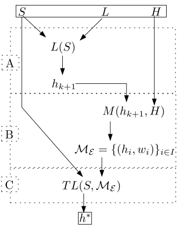
It might be asked what the position of the algorithm for inducing the transfer is, in relation to item d) above and traditional algorithms. In Figure 2.2 the flow of a implementation of this framework is shown.

As shown there, we can consider the base-learning algorithm (L), the algo-rithm cooking up the hypotheses (M) and the transfer learning (TL) algoalgo-rithm separately. In a sense this is a wrapper framework, as it is not dependent on the specific implementations. This we state as Algorithm 3, Transfer Inducer (TI), which encapsulates what is shown on Fig. 2.2. We’ll refer again to this figure when discussing the experiments.

2.3

A Meta-Algorithm

With the communication scenario from the previous section in mind, we now state a meta version of the algorithm, as given in Alg. 1, 2 and 3.

In Algorithm 1 we like to keep the h_k+1 separate for convergence reasons discussed later.

Algorithm 1: (M) A hypothesis grinder/combiner; partitions the knowledge contained in a hypothesis into simpler hypothesis allowing for combinations and assigns prior weights to each hypothesis. This function should resemble a cognitive process

input : A set of hypothesesH={h1, . . . , hk}, and a special

hypothesishk+1

output: M_E ={(hi, wi)}i∈I

% find more general hypothesis M∗

1←chop(H)

M∗

2←chop(hk+1)

% eachhi∈ ME gets weightwi=n1·wA+n2·wB,ni the number of

occurrences ofhinM∗_i, i.e. how many instances ofhthere are inM∗_i ME ←combine((M∗1, wA),(M∗2, wB))

% Notes:

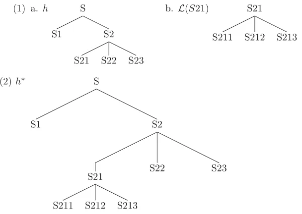
chop: this function “chops” the knowledge contained in a hypothesis into components of less complexity, which constitute the output, making it more general in the process since it covers less cases then the original hypothesis. This function should not go beyond it’s input; i.e. the union of all its outputs should be a subset of the input. The term “chop” comes from how this function might behave on decision trees, where we would chop the tree into subtrees.

Algorithm 2: (TL) Scheme for inducing transfer from a hypothesis-collection and a dataset

input : A set of hypothesisM_E ={h₁, . . . , h_n} with associated weights w_i, learning algorithmLwith the same hypothesis representation asM_E , datasetS

output:h∗: MDL hypothesis overM_E w.r.t.S

%codelength of each hypothesis fori←1 tondo

lh[i]←LC(hi)

end

lh[n+1]←LC(hi)

%codelength of data, given each hypothesis fori←1 tondo

lDh[i]←LC(S|H)

end

%(weighted) total codelength fori←1 tondo

tLC = lDh[i] + w[i]*ld[i] end

S

L

H

L

(

S

)

h

M

(

h

, H

)

M

=

{

(

h

, w

)

}

T L

(

S,

M

)

h

A

C

B

Figure 2.2: Relation between types of algorithms that appear in this paper, which can be considered as a Transfer Inducer (TI, Alg. 3). H is a collection of hypotheses h, L is a learning algorithm, S is a dataset, M is a hypothe-sis induction algorithm, that might for instance make partial hypotheses from those contained in H, and TL evaluates hypothesis for transfer producing a single most probable hypothesis h∗. The A part of the figure corresponds to ordinary learning, B to hypothesis space construction and C to the transfer learning/evaluation.

thought of as mappings from the priorP(H)to a new priorP(H)1/(f+1)_{, where}

f is the frequency of the hypothesis in M, assigning f = 0 to the hypotheses constructed from Sk+1. Thus, w(Lk+1(Sk+1)) = 1, and another hypothesis

h occurring once would get w(h) = 1/2, and so forth, by the correspondence between codelengths and probabilities. The essence of transfer to the new task is captured by these weights. Contrary to the approach in Statistical Learning Theory, where the model is penalized by someregularization factor to prevent overfitting, we discount the models that the environment indicates are more probable.

In [Zha04] and [BC91] a modified information complexity minimization

crite-Algorithm 3: (TI) A transfer inducer; wrapper for the framework in fig. 2.2.

rion7_{is studied where the model complexityL(h)is assigned someregularization} parameter λ. The contribution of the model complexity to the total then be-comes λL(H). This λ is used in a similar way as our w and has been shown to make the estimation method more robust for λ >1. Unfortunately, neither paper offer any intuitive interpretation of this parameter and it only serves a technical purpose to improve the bounds derivable. In this case, the ends justify the means. It is not clear from either paper why, besides the technical justifi-cation, we should allow for this parameter and sparse advise is offered on the value to assign to λ.

The relevance of these results for our work is that it might be advisable to use w(H) > 1 for all hypothesis. However, that undermines the purpose of transfer, namely to adopt more complex hypotheses then the data alone give rise to, as indicated by the environment.

Zhang’s results imply for us, that we put not too small of a prior weight on a hypothesis that is close to the “truth” (even if such a hypothesis is not in the space under consideration), so we should take care not to assign too low weight to the empirical distribution, the distribution constructed form the new task, since in general we expect the underlying learner to be convergent.

Since we have not included any information on the size of the dataset used for constructing the hypotheses we would like substructures from each learner (domain) to be available, since we may only have very limited data in Sk+1.

What sort of structures might these be?

One particularly appealing thing to do in Alg. 1 with the elements of H, the set of given hypotheses, is to construct less specific hypotheses from, i.e. hypotheses based on fewer features and with fewer partitions of the input-space. These hypotheses would represent a subset of the knowledge contained in each hypothesis, allowing the algorithm to refrain from over generalizing based on the limited data inSk+1and adopt a subset of the knowledge contained in each

hypothesis. Another appealing thing to do with the hypotheses is to join disjoint hypotheses, allowing for overlap between two or more domains; specifically this might be useful based on restricted hypothesis. We illustrate how this might proceed in Section 4.4.

To use this algorithm we need to instantiate all the steps in the procedure, which we give an example of in Chapter 4 using decision trees. The issue of coding the relevant structure for the inference is usually quite tricky, but for a decision tree implementation it turns out to be rather straight forward, see 4.2.

2.4

Discussion

Here we discuss the minimization of the code length for the environment as a whole. In all cases, we have a new, previously unseen task to solve, given a new datasetSk+1, and the environment knowledgeME. The question addressed in

this section is what to optimize.

If we have available the datasets Si, i ∈ {1,2, . . . , k}, k ∈ N, from the

do-mains used to construct the hypotheses inME, a sensible thing to do would be to consider the new task as a part of the environment and solve:

arg min

H

The hypothesis H∗ minimizes the total codelength for the whole environment. If the datasets are not available, as we assume in this paper, we can consider two distinct minimization problems to solve when finding an optimal hypothesis for the new task. The first is the one considered in this paper:

arg min

H∈ME

{w(H)L(H) +L(Sk+1|H)},

where the weightsw(H)are given positive reals and adjusted to allow for more complex models then the data alone would.

The other might be formalized as follows. Still, ME is fixed, but there is no need for specifying the weightsw(H). From the environment knowledge, we find the optimal hyper-hypothesis or-prior:

arg min

h∈Θ {

L(h) +

j

L(Hj|h) +L(Sj|Hj)}= arg min

h∈Θ {

L(h) +

j

L(Hj|h)}=h∗a,

since the terms L(S_j|H_j)does not depend on h; Θis the space for the hyper-prior. Then, when we get new dataS_k+1, which we consider to be a part of the environment abstractly described byh∗_a, we solve

arg min

H {

L(h∗_a) +L(H|h_a∗) +L(Sk+1|H)}= arg min

H {

L(H|h∗_a) +L(Sk+1|H)},

to get the optimal description of the new data, when assuming that it originates from the same environment.8 _{To apply this method, we need to specify the} hyper-prior, or a code length function for the hypotheses fromΘandL(H|h∗_a), which does not appear to be obvious. This approach could be termed three part MDL, and has close relations with the hierarchical Bayes method.

The approach taken in this paper appears to be more robust to misspecifica-tion of the environment then when specifying a hyper-prior. Misspecificamisspecifica-tion of the prior would affect the codelength of the hypothesis given the hyper-prior in a adverse way. The alternative optimization outlined in this section does not concentrate on the new task, but on the environment as a whole when viewing the new task as a part of it. It might be said that the method with the weights concentrates on performing well on the new,current task, while the other approach, outlined in this section, concentrates on finding good abstrac-tions based on everything in the environment. One finds good predicabstrac-tions for what happens next, the other constructs good models of the environment. If there is even one domain that doesn’t group well with the other tasks9_{then the} abstraction might be “confused”, while the method we devote this paper to does not get so easily confused. It would seem that our method, with the weights, concentrates on performing well on the new task, while the other on any unseen task. The latter case is addressed in [Bax00]. Are these problems distinct? Is the three part description length minimization better then weighing the prior knowledge? A proof that our approach is better or not then the three part MDL approach would be nice, but that is the subject of another paper.

In short, which optimization problem we solve, and what we assume, depends on the purpose of our investigations: are we learning about the environment or learning to solve the new task? In this paper, we concentrate on performing well on the new task.

8_{This is slightly reminiscent of the expectation-maximization (EM) method [DLR77].}

Which learning algorithms? So far we have assumed that all learners are using the same learning algorithm. Now we ask: what restrictions should be imposed on the learners producing the hypotheses in M_E? Basically the only restriction is that we have a coding scheme to produce the codelengths of the hypothesis so we can evaluate if the hypothesis is transferable or not. We are not concerned with how the hypothesis are made, only whether they are useful or not for the task at hand.

Taking a closer look at the framework, another thing reveals itself. The usefulness of the hypotheses inME, as measured by the transferability, can be influenced by the construction of the hypothesis. But, if the hypotheses are bad that will be reflected in poor transferability.

Further, we can repeatedly apply the TI algorithm to unexplained data, until the transferable set is exhausted.

No Free Lunch and Transfer learning Researchers are sometimes con-cerned with No Free Lunch (NFL) style results, see [WM95]. These results rely on the premise that all inputs are equally likely a priory, observations are i.i.d. and the problem spaces are finite, which is rarely the case. As concerns our algorithm, the bias of the underlying algorithm is enriched with information from an environment, which further directs the search for an optimal hypothesis away from any sort of uniform prior.

Chapter 3

Convergence

“The truth is not out there.”

— Not Agent Mulder from the television show The X-files.

In this chapter we address the asymptotic properties of our method. Why do we need asymptotic properties? Without those we can’t state that our method is actually of any use. If more data isn’t of use for our method, then it wouldn’t really be adjusting to the properties of the data, or to the structure indicated by the data. We are looking for algorithms that learn from data, so this is essential. Asymptotic properties, however, do not necessarily tell us anything about small sample properties: in practice these are the properties of real importance.

To provide formal grounds for the utility of our method we need theorem 3.2.4 which gives bounds for the divergence of a probability measure from atrue measure. Loosely speaking, this theorem tells us that if the true measure, or classifier, is in the collection of hypotheses Mthen our method will recover it eventually. This result hinges on the learning problem being realizable, using MDL as the basis of inducing transfer and the underlying method being con-vergent. These asymptotic results give us a guarantee of the behaviour of the proposed framework but do not state anything about restricted size sample re-sults It may very well be that a suspicious looking hypothesis will be selected for transfer based on a sample, but eventually (in mean sum, as defined later) when there is enough data, a wrong bias on the hypothesis space will be overcome. In the end, there is only the data to base inference on.

The convergence results are due to Hutter and Poland [HP05] but adapted to cover only our present setup, with some simplifications and more detail then in the original paper. Their work draws on Solomonoff’s seminal paper [Sol78], containing results from 1968(!), where he proves for the Bayes mixture distri-bution ξ over any collection of measuresC containing the true distributionμ,

ξ(x) =_ν∈Cwνν(x), that

∞

t=1

E

a∈X

(μ(a|z)−ξ(a|z))≤lnw_μ−1.

where z is sequence from X∗1_{, and an earlier paper by Hutter [Hut01] with} 1_{An interesting account by Solomonoff of discoveries can be found at}

results from 1999:

∞

t=1

E

a∈X

(μ(a|z)−ρnorm(a|z))≤w−μ1+ lnwμ−1,

where

ϕ_norm(a|z) =_def ϕ(a|z)

bϕ(b|z)

=ϕ(za)

bϕ(b|z)

for any functionϕ:Zn →[0,1],n∈N, wherezais the sequencezwithaadded to the end. The result we need is the convergence between the true measure and a MDL predictor, which will be defined shortly.

This chapter is on the technical side but is nevertheless important since without asymptotic statements about our algorithm we don’t know if they are of any use.

3.1

Convergence Concepts

The proofs of convergence given in Section 3.2 are based on the concept of convergence in mean sum. This we relate to the more familiarconvergence in probability, which is the probability theory equivalence of the measure theoretic almost everywhere.

The following convergence concepts are of interest:

Definition 3.1.1 A sequence of random variablesx1(ω), x2(ω), . . .fromΩ

con-verges to x(ω),xi: Ω→R

in probability iflim_t→∞P({ω∈Ω :|xt(ω)−x(ω)|> ε}) = 0

with probability one ifP({ω∈Ω : lim_t→∞xt(ω) =x(ω)}) = 1

in mean sum (i.m.s.) ∞_t=1E[(xt(ω)−x(ω))2]<∞

where P is a probability measure. Convergence with probability one is also re-ferred to as almost sureand almost everywhere convergence.

Almost sure convergence is frequently used in probability theory and is the concept used in the strong law of large numbers, which states that a sample average tends to the mean of the distribution generating the observations almost surely, loosely speaking.

These concepts are related by the following lemma, which shows that the i.m.s. concept is the strongest of the three:

Lemma 3.1.2

1. Almost sure convergence implies convergence in probability.

2. Convergence in mean sum implies almost sure convergence .

Proof See [Ser80].