Evaluation tool for demand side management of domestic hot water load

(1)

Evaluation Tool for

Demand-Side Management of

Domestic Hot Water Load

by

Wong Koon Kong, BEng (Hons)

Submitted in fulfilment of the requirements for the Degree of

Master of Engineering Science

School of Engineering

University of Tasmania

(2)

(3)

Declaration of Originality

This thesis contains no material which has been accepted for a degree or diploma by the University or any other institution, except by way of background information and duly acknowledged in the thesis, and to the best of my knowledge and belief no material previously published or written by another person except where due acknowledgement is made in the text of the thesis, nor does the thesis contain any material that infringes copyright.

……….. Wong Koon Kong

Date: 02 September 2014

Statement of Authority to Access

This thesis may be available for loan and limited copying and communication in accordance with the Copyright Act 1986.

……….. Wong Koon Kong

Date: 02 September 2014

(4)

Preface

Abstract

This thesis presents the development of an evaluation tool for demand-side management (DSM) of domestic hot water systems (DHWSs). The developed tool provides accurate modeling and predictions of potential peak demand reductions through direct control of DHWSs. It aims to assist distribution system operators (DSOs) in designing a DSM program to deliver desired peak load reductions while maintaining a satisfactory level of comfort for all consumers.

The developed tool estimates the available domestic hot water load in a controlled area, and determines optimal switching programs for direct load control (DLC). A switching program refers to a direct control schedule that strategically switches DHWSs on and off in order to achieve a desired load reduction during peak periods.

To calculate the power consumption and temperature profile of a DHWS, we developed a multi-layer thermally stratified hot water system model and validated it with experimental data. The tool employs Monte Carlo probabilistic simulations to generate hot water consumption profiles for domestic consumers, and uses the hot water system model to obtain the loads associated with these hot water consumption profiles. Switching programs for DLC found via iterative optimizations, are applied to these hot water loads to meet the peak reduction targets set by the tool user. Key performance indicators (KPIs) to evaluate the performance of these switching programs and the impact on consumers’ comfort as a result of implementing DLC, were also developed.

(5)

Outline of the research

This research focuses on DLC of DHWSs, as a DSM approach to reduce the peak domestic load in a power distribution network. DHWS is chosen as the control target of this research for two main reasons:

• The domestic hot water load represents a significant share of the total domestic energy load. Water heating accounts for up to 40% of domestic energy consumption in Australia and approximately one third in Tasmania [1], [2]. Hence, a DLC program that can effectively reduce the peak domestic hot water load will have a significant impact in reducing the peak load of the substations. For example, Integra Energy (New South Wales, Australia) has successfully reduced its system peak demand by 389 MW through implementing DLC on DHWSs [3].

• A DHWS represents an interruptible load because it is an insulated thermal energy storage that continually supplies hot water to consumers even during the period of power interruptions. The deferred energy is recovered when the power is restored. Hence, a well-designed DLC program has a minimal impact on consumers’ existing comfort levels.

This research has two main objectives:

1. To develop a domestic hot water evaluation tool that can accurately model the available hot water load and predict the potential peak reduction achievable through direct control of domestic electric hot water systems.

2. To use the developed tool to assist distribution system operators in designing their load management (LM) programs, with the aim of delivering optimal peak reduction in domestic loads while ensuring minimal impact on consumers’ existing comfort levels.

Achieving these objectives requires research in the areas summarized below:

1. Develop an accurate model to predict the power consumption and temperature profile of a domestic electric hot water system.

2. Develop a generic approach to estimate hot water consumption profiles in individual households.

(6)

3. Derive a set of key performance indicators to measure, evaluate and compare the performance for various controlled scenarios.

4. Develop a control management system that produces DLC switching programs and employs effective algorithms to optimize them. These switching programs are applied to the DHWSs to reduce the aggregate peak load and improve the load factor.

5. Develop a user-friendly program that integrates the above functions into a tool that assists the DSOs in the evaluation and selection of DLC switching programs for their respective load management purposes.

Figure (I) shows the block diagram that summarizes the research objectives and the research areas to achieve these objectives.

Figure (I) Block diagram illustrating research objectives and research areas.

With reference to the research areas discussed above, this thesis is organized as follows:

Chapter 1 provides an introduction to DSM. This chapter contains a general overview of the history of DSM, the implementation of DSM in some major countries, a review of methods and strategies to implement DSM, and values of DSM in an electric power system.

(7)

Chapter 2 presents the structure of the developed hot water evaluation tool. It introduces the high level structure of the tool and describes the functionality of individual modules in the tool. In addition, the high level operation of these modules and the flow of information between them are also discussed. Detailed descriptions of the main functional modules are provided in the following chapters.

Chapter 3 outlines the generic approach in the estimation of domestic hot water consumption profiles in Tasmania, Australia. It presents the Monte Carlo approach employed to generate hot water consumption profiles for individual households. Survey results, actual energy metering data, and demographic data are used in the estimation process. As a result, the estimated hot water consumption profiles are correlated to the demography and the consumer behavior in the controlled area. The operation of the hot water consumption generator module is described in this chapter.

Chapter 4 presents the development of the domestic hot water system model. This chapter provides the mathematical modeling with heat energy equations of the most common DHWS in Tasmania. Furthermore, the validation with experimental data is also presented.

Chapter 5 describes the operation of the performance calculator and the details of the control management system. This chapter defines the KPIs used by the tool to evaluate the performance of DLC switching programs, as well as describing in detail the optimizer module and algorithms developed to optimize DLC switching programs.

Chapter 6 evaluates the developed tools with a number of case studies. The studies assess the scalability of the results, impacts of assuming certain parameters as constant in simulations, as well as the performance of different DLC switching programs applied to DHWSs under different operating scenarios. In addition, this chapter also includes discussions of the simulation results.

Chapter 7 summarizes the research and gives some recommendations for future studies aiming to extend the research work reported in this thesis.

(8)

Publications

Journal and conference papers given in the following list have been produced as the outcome of this research.

Journal papers

1. M. Negnevitsky and K. Wong, "Demand side management evaluation tool," IEEE Trans. Power Syst., vol. 99, pp. 1-11, 2014.

2. M. Negnevitsky and K. Wong, "A practical approach to modelling of domestic electric hot water systems for load management programs," Applied Thermal Engineering, under review.

Refereed conference papers

1. K. Wong and M. Negnevitsky, "Development of an evaluation tool for demand side management of domestic hot water load," in Proc. IEEE PES General Meeting, 2013, pp. 1-5.

2. K. Wong and M. Negnevitsky, "Optimisation of switching programs for demand side management of domestic hot water load," in Australasian Universities Power Engineering Conf., 2013, pp. 1-6.

(9)

Acknowledgements

First of all, I would like to express my deep gratitude to my supervisor, Professor Michael Negnevitsky. I thank you for being a great mentor to me. I appreciate very much your patience, and the advice and motivation you have given me throughout my research. I would also like to thank Dr. Osman Haruni for all the significantly useful and constructive discussions we had during the early stage of my research. Furthermore, I wish to say thank you to all the technical staff in the School of Engineering, especially Calverly Gerard, James Lamont, Peter Seward and Andrew Bylett, who helped me in setting up the test system in the laboratory.

In addition, I wish to thank Aurora Energy, Australia for providing the financial support and the survey data required in my research. I also gratefully acknowledge Peter Milbourne, James O’Flaherty, Daniel Capece, Cherry Wynn and Dr. Thanh Nguyen of Aurora Energy for productive discussions of the results presented in this thesis.

A special thanks to my fellow postgraduate researchers at the School of Engineering, especially Dinh Hieu Nguyen, Zane Smith, Sarah Lyden and Ahmad Tavakoli. We had a great number of positive discussions which were helpful to my work.

Lastly, I would like to thank my family and loved ones. My research work has only been possible with your support and love.

(10)

List of tables

3.1 Correlation between average number of showers and family size ... 27

3.2 Time intervals between two consecutive recharges due to standing heat losses from the hot water storage tank, for two sets of common parameter values ... 32

3.3 Family types and their distributions in a controlled area ... 34

3.4 Probabilities for shower schedules to occur in the morning only, evening only and both 34 3.5 Probabilities of number of showers in a shower schedule for each family type ... 34

3.6 Default values for shower lengths and gaps between consecutive showers ... 35

4.1 Assumptions applied in the formulation of the DHWS model ... 46

4.2 Operating conditions and configurations of the test system in three measurements ... 55

4.3 Physical parameters of the DHWS model used for Simulations 1, 2 and 3 ... 55

4.4 Operating conditions of the DHWS model in Simulations 1, 2 and 3 ... 56

4.5 Values of Pmean used in Simulations 1, 2 and 3 ... 56

4.6 Prediction errors of Simulations 1, 2 and 3 compared to Measurements 1, 2 and 3, respectively ... 64

5.1 Control management system parameters ... 77

6.1 Results of comparative analyses ... 87

6.2 Default switching program configuration ... 91

6.3 Control periods and peak reductions for UDCP and OCP optimizers ... 92

6.4 Probabilities of cold showers for uncontrolled scenario and controlled scenarios ... 93

6.5 Probabilities of cold showers for a hot water load profile with dominant afternoon peak under uncontrolled and controlled scenarios... 94

6.6 Switching program configurations used in the case studies ... 95

6.7 Probabilities of cold showers for uncontrolled scenario and controlled scenario employing switching configuration 2... 95

6.8 Probabilities of cold showers for uncontrolled scenario and controlled scenario with maximum control periods ... 97

(14)

List of figures

1.1 Average daily total load profile in winter months of a substation in Tasmania dominated

by domestic load. ... 2

1.2 Block diagram of main components in DSM. ... 5

1.3 The simplified structure of a deregulated power system. ... 13

1.4 Monthly availability factor for four high-wind stations in Taiwan [47]. ... 14

2.1 Overall structure of the hot water evaluation tool. ... 18

2.2 Main GUI of the hot water evaluation tool. ... 19

2.3 An error message due to the entered value being outside of the valid range. ... 20

2.4 A warning message due to the entered value being outside of the expected range. ... 21

2.5 GUI for viewing or changing physical parameters of DHWS. ... 22

2.6 GUI for viewing or changing operating conditions of a DHWS. ... 22

3.1 Average number of showers versus the number of residents per household. ... 26

3.2 Histogram of the average duration of showers. ... 27

3.3 Distribution of types of DHWS among the surveyed households. ... 28

3.4 Probability distribution of the starting time for showers, smoothed by moving average. . 29

3.5 Probability distribution of starting time for low volume usages derived directly from energy metering data. ... 30

3.6 Filtered and processed probability distribution of starting time for low volume usages. . 32

3.7 Block diagram of the hot water consumption generator. ... 33

3.8 A typical hot water consumption profile of a household. ... 33

3.9 Cumulative probability distribution of starting time for showers. ... 36

3.10 Flow chart showing main operations of the hot water consumption generator. ... 37

3.11. Average hot water consumption profiles for family type 1 to type 4. ... 38

3.12 Aggregate hot water consumption profile for all family types... 39

4.1 Simplified block diagram of DHWS. ... 40

4.2 Schematic diagram of a tempering valve [54]. ... 42

4.3 (a) thermally stratified hot water storage tank; (b) well-mixed hot water storage tank. ... 43

4.4 Block diagram of a hot water storage tank divided into mixing zone and layer zone... 45

4.5 Block diagram of a tempering valve. ... 47

4.6 Vertical temperature profiles of a hot water storage tank: (a) before a draw, (b) after a draw [63]. ... 49

4.7 States of the hot water storage tank, (a) before heating model is applied, (b) after heating model is applied. ... 52

(15)

4.8 Test system setup for model tuning and validation. ... 52

4.9 Illustration of shower schedules in 48 hours. ... 54

4.10 Top layer temperatures over 48 hours for Measurement 1 and Simulation 1. ... 57

4.11 Normalized power consumptions over 48 hours for Measurement 1 and Simulation 1. 57 4.12 Normalized cumulative hot water consumptions over 48 hours for Measurement 1 and Simulation 1. ... 58

4.13 Shower temperatures in shower schedule 1 for Measurement 1 and Simulation 1. ... 58

4.18 Normalized power consumptions over 48 hours for Measurement 2 and Simulation 2. 60 4.19 Normalized cumulative hot water consumptions over 48 hours for Measurement 2 and Simulation 2. ... 61

4.24 Normalized power consumptions over 24 hours for Measurement 3 and Simulation 3. 63 4.25 Bottom layer temperatures over 24 hours for Measurement 3 and Simulation 3. ... 63

5.1 Block diagram of switching program optimizer... 73

5.2 A typical switching program and its control management system parameters. ... 75

5.3 Block diagram of the UDCP optimizer. ... 76

5.4 Oscillations in aggregate controlled load curves produced by the UDCP optimizer. ... 77

5.5 Aggregate controlled load curve without oscillations produced by UDCP optimizer. ... 78

5.6. Aggregate controlled load curve produced with PI functions in UDCP optimizer. ... 78

5.7. Initial control period in relation to LT and LU. ... 79

5.8 Scenario 1, 2 and 3 used in OCP optimization. ... 80

5.9 OCP optimization results for iteration 1 and iteration 6. ... 82

6.1 Uncontrolled load curves with dominant morning peak for 1500 households. ... 85

6.2 Uncontrolled load curves with dominant evening peak for 1500 households. ... 86

6.3 Uncontrolled load curves with dominant morning peak for 3000 households. ... 86

6.4 Uncontrolled load curves with dominant evening peak for 3000 households. ... 87

6.5 Average ambient and cold water temperatures in winter time. ... 88

(16)

6.6 Uncontrolled load curves for constant and variable values of ambient and cold water

temperatures. ... 89

6.7 Uncontrolled load curves for constant and variable turn-on and turn-off temperatures. .. 90

6.8 Result of the UDCP optimization... 92

6.9 Result of the OCP optimization. ... 92

6.10 The OCP optimization of a hot water load profile with a dominant afternoon peak. ... 94

6.11 The OCP optimization with switching program configuration 2. ... 96

6.12 The OCP optimization result with control periods limited to 7.5 hours. ... 97

(17)

List of abbreviations

AC Air conditioner

AMI Advanced metering infrastructure CLM Conservation and load management CO2-e Carbon dioxide equivalent

CPP Critical peak pricing

DCCEE Department of climate change and energy efficiency DG distributed generation

DHWS Domestic hot water system DLC Direct load control

DRED Demand response enabling device DSM Demand-side management

DSO Distribution system operator ERF Error function

EU European Union GUI Graphical user interface I/Os inputs and outputs

KPI Key performance indicator LM Load management

MAE Mean absolute error

MAPE Mean absolute percentage error NEM National Electricity Market OCP Optimized control period PI Proportional and integral RMSE Root mean square error RTP Real Time pricing

SWIS South West Interconnected System ToU Time of use

TSO Transmission system operator UDCP User defined control period

(18)

List of symbols

The following is a list of key symbols used in the thesis. Other symbols are introduced and described within the texts where they first appear.

HL Height of the entire layer zone measured from the top of the mixing zone. Kp Proportional gain of the PI functions.

LC Aggregate controlled hot water load curve.

LT Target peak value for aggregate controlled hot water load. LU Aggregate uncontrolled hot water load curve.

N Number of stratified layers inside a hot water tank. NH Total number of households.

NS Total number of Monte Carlo iterations. P Rated power of the hot water system. Pcold Probability of cold showers.

R(τ) Peak load reduction in control period specified by τ. Ta Ambient temperature.

Tc Cold water temperature.

tf Finishing time of a control period. ts Starting time of a control period. Ti Integral time of the PI functions.

Tj Temperature of layer j inside a hot water tank.

Tmz Mean temperature of the mixing zone in a hot water tank. Toff Thermostat turn-off temperature.

Ton Thermostat turn-on temperature. Tshwr Shower temperature.

W¯ Aggregate hot water consumption profile of a controlled area. w(i, j) Hot water consumption profile of household i in iteration j. Zj Height of layer j inside a hot water tank.

α The ratio of hot water flow to mixed water flow of a tempering valve τ Control period in a switching program.

τoff Turn-off period in a switching cycle. τon Turn-on period in a switching cycle. τsc Switching cycle in a switching program. τstep Control step in a switching program.

(19)

Chapter 1 Introduction

Electricity is a form of energy that is very costly to store in bulk with existing technologies. For example, the global energy storage capacity represented just 3% of the global generating capacity in 2010 [4], [5]. Hence, most of the time, electric energy is consumed as it is generated. Moreover, the demand for electricity is not consistent but exhibits daily and seasonal variations. These unique characteristics present major challenges in designing and planning for an electric power system1.

In order to ensure a high level of supply availability, the capacity of an electric power distribution system is traditionally designed to support the peak load forecast in the network [6], [7]. Although this design approach is essential in minimizing supply interruptions, it creates excessive latent capacity in distribution networks with low load factors (ratio of average to peak load). This scenario represents inefficient utilization of network infrastructures. As an example, the cost of catering to peak loads has caused electricity prices to double in Australia over the last five years [7]. Capital expenditures of close to half of the total network investment and more than half of the transmission budget are spent to accommodate the peak load growth in the National Electricity Market (NEM) in Australia. This amount accounts for about A$10 billion in system capacity that is used for slightly more than one percent of a year [8]. Similar costly underutilization is reported in the South West Interconnected System (SWIS) of Western Australia. To meet peak demands in 2009, about 600 MW (or 12 %) of capacity in the SWIS was used for less than one percent of the year [9].

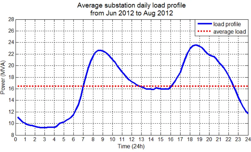
The characteristic of low load factor is commonly evident in domestic load profiles. The peaks are usually seasonal and persist only for a few hours of a day. For the rest of the time, the load is considerably lower than the peaks. For example, Figure 1.1 shows the average daily load profile (for winter months) of a substation

1_{“Power”, unless explicitly stated otherwise, means “electric power” in this thesis.}

(20)

Chapter 1: Introduction

[image:20.595.91.499.220.467.2]

serving residential areas in the Tasmanian (Australia) distribution network. The majority of this substation’s loads were domestic demands. Its load factor (ratio of average to peak load) was about 0.7, and the load was below its average value for more than half of the time. The summer load in Tasmania is relatively lower than its winter load.

Figure 1.1 Average daily total load profile in winter months of a substation in Tasmania dominated by domestic load.

To overcome the problem of low efficiency in a power system, such as those in the aforementioned examples, active initiatives are needed to reduce peak loads, improve the load factor and enhance the overall network utilization. One of the widely implemented initiatives is DSM — the effort to reduce energy consumption and improve the overall power system efficiency through the implementation of policies and methods that modify consumer demand for electricity [10]. The following sections provide a review of DSM. Section 1.1 gives a brief overview on the history of DSM and its implementations in three major countries. Sections 1.2–1.4 describe different types of DSM initiatives and how they are implemented around the world. Section 1.5 discusses the values of DSM implementations in modern power systems.

(21)

1.1 Overview of Demand-side Management

The initial concept of DSM was coined during the Arab oil embargo in the early 1970s where the price of crude oil had quadrupled overnight from about US$2.50 to US$10.00 per barrel [11]. This incident had prompted an urgent requirement in the USA and other western countries for energy conservation programs to counter the adverse impact of the sharp rising cost in power generations. The early DSM programs in the USA were known as “conservation and load management” (CLM) [12]. At the same time, consumers responded positively to the DSM initiatives of the utilities under such circumstances.

Analysis made in [11] divides implementations of DSM in the USA, from its inception in the early 1970s to 1994 and onwards, into three phases. The first phase (from 1973 to the late 1980s) occurred in the period of high oil prices and DSM initiatives were implemented mainly to conserve energy and to reduce generation costs. When oil prices tumbled in the late 1980s, the DSM implementation entered its second phase where regulatory bodies had to provide incentives for the energy and utilities sector to continue pursuing DSM opportunities. The third phase began after the deregulation of the energy market in the USA in the 1990s where competition and market forces became the dominant drivers in DSM programs. Among other states in the USA, California (CA) and Vermont (VT) have very cost-effective DSM implementations [13]. Through its energy efficiency agency, VT has successfully reduced about 50% of the growth on its electricity load. Meanwhile, energy efficiency and DSM programs implemented in CA enabled that state to maintain almost constant electricity consumption per capita for the period between the early 1980s and 2004, while the rest of the USA had an average rise of about 50% in the same period [13].

To curb rising carbon emissions and the growth in energy intensity, the Chinese government has set an aggressive goal to reduce 20% of energy consumption per GDP for the period between 2005 and 2010 [13]. DSM initiatives are among the major initiatives to achieve this goal. Currently, DSM initiatives in China’s power systems are primarily under central control. Studies in [14] reveal that the Chinese government has allocated an equivalent of US$3.08 billion to improve energy efficiency and to reduce pollution. As a result, reforms institutionalized at all levels

(22)

of government are expected to have long term positive effects in improving the energy efficiency for China.

Studies in [15] and [16] reveal that back in 2009, India faced major issues in its energy supplies. Its energy deficit was about 10%, while the shortage in peak capacity was about 13%. The Indian government enacted the Energy Conservation Act in 2001 to promote energy efficiency and conservation [16]. Plans to use more energy efficient devices and equipment represent the major DSM initiative for significant energy conservation in India [15]. DSM is estimated to potentially reduce peak demand in the range of 837 – 4,904 MW, and save energy in the range of 3,311 – 17,852 GWh. However, ineffective tariff systems hamper the effort to implement effective DSM programs in India, specifically its agricultural sector dominated by energy inefficient irrigation pumps.

1.2 Main Types of Demand-side Management Initiatives

Since its inception in the early 1970s, DSM is currently getting considerable attention in modern power systems around the world. The study conducted in [17] attributes the resurgence of DSM efforts in recent years to growing concerns over climate change, volatile fuel prices and shrinking utility reserve margins. Figure 1.2 shows the three major types of DSM that require different efforts to implement in a power system [17]. They are summarized below:

• Improve energy efficiency through technical advancements such as usages of energy efficient devices and equipment, upgrades of insulation, applications of enhanced building materials etc. Active consumer participation is expected to have a positive impact on the success of this DSM effort.

• Change demand profiles through LM programs that apply various methods of control mechanisms such as direct load control, autonomous demand response etc. • Promote energy conservation through educational programs and financial incentives that alter consumer behavior to reduce wastage and conserve electricity [18]. The behavioral changes may be short term or become long term if they are incorporated into the lifestyle of a population [19].

(23)

The first two methods of DSM are further discussed in the following sub sections.

Figure 1.2 Block diagram of main components in DSM.

1.3 Energy Efficiency Programs

Energy efficient programs refer to initiatives that promote the permanent installation of energy efficient technologies and the elimination of energy losses in the existing system [19]. This section looks at the DSM policies and methods employed in some countries to improve energy efficiency in power systems.

Comprehensive analyses in [20] present the policy options in improving energy efficiency in Australia. Among other recommendations, this report proposes a multi-stage market reform that encompasses energy sectors and other related sectors such as building industry, commercial and industrial equipment sectors etc. To have long term effective results, the report also proposes to incorporate the energy efficiency criteria into future policies.

A number of DSM initiatives in stimulating technical changes to improve energy efficiency are discussed in [21]. These methods include encouraging the dissemination of energy efficient appliances through subsidy programs and comparison labeling, eliminating least efficient devices through standardization, and

(24)

advancing new technologies and innovations in energy efficiency through incentive. This paper provides the success story of comparison labeling in Australia where the sales of more energy efficient appliances have successfully reduced the average household energy consumption by 11% in 1992. Through standardization of efficiency for household appliances, Lawrence Berkeley Laboratory in the USA projected an energy saving of 7,000 TWh from 1990 to 2015 and an avoided power generation of about 21,000 MW in 2015 for the USA [21].

Meanwhile, research in [22] reports that national standards on minimum efficiency of appliances adopted in the USA have successfully cut electricity consumption by 88 TWh (equivalent to 2.5% of national electricity usage) in the year 2000. This paper also reports a projected energy saving of 0.35 EJ (equivalent to 97.2 TWh) by 2010 in Japan, from the revision of the Energy Conservation Law in 1998. This law introduces minimum energy performance standards for household appliances and promotes innovations in energy efficient technologies. Under the same law, the authors of [19] reports that energy-intensive industrial facilities in Japan are required to reduce their respective energy intensities by 1% annually. From reported statistics, about 52% of these facilities met the target in 2004.

Multinational energy efficiency policies adopted by the European Union (EU) countries in the 1990s have reduced the energy consumption of washing machines and dishwashers by 20%, and refrigerators and freezers by 27% [22]. In the case of China, the investments in end user devices with high efficiency have saved about 579 MW of generation in the Jiangsu province power system [10].

On the other hand, DSM initiatives to promote energy efficiency are sometimes perceived negatively as reduced revenue for the energy and utilities sector. Hence, regulatory or governmental incentives are occasionally required to support such initiatives. The study in [23] analyses the world’s first trading scheme for energy efficiency certificates (“white certificates”), which commenced in New South Wales, Australia in January 2003. The findings discover that this trading scheme represents an effective mechanism for incentivizing the abatement of greenhouse gas emissions. An equivalent of about 10 million tonnes of carbon dioxide equivalent (CO2-e)

abatement was achieved by the end of 2006.

(25)

1.4 Load Management

Conventionally, LM represents various control methods that are applied to change the consumer demand profiles. As shown in Figure 1.2, there are three methods to implement LM in a power system:

• Indirect load control • Autonomous load control • Direct load control

1.4.1 Indirect load control

Indirect load control refers to demand response schemes that require active participation of consumers to make manual adjustments to change their respective consumption profiles. This LM method is usually associated with various time-sensitive pricing schemes such as time of use (ToU) pricing, real time pricing (RTP) and critical peak pricing (CPP) [24]. A common application of this LM method is the off-peak tariff for heating hot water storage tanks [25]. In a deregulated power sector, indirect load control relies strongly on market forces for effective demand responses during peak demand periods where the costs of electricity are the highest [26]. The research in [27] estimates the potential peak load reduction in the California (CA) power system via indirect load control of domestic air conditioner (AC) loads responsive to the RTP of electricity. In the case study presented, adjustment of the indoor temperature range between 68oF (20oC) and 72oF (22.2oC) is reported to shift more than 80% of energy consumption on AC during a peak period to non-peak periods, as compared to maintaining a constant indoor temperature at 70oF (21.1oC) throughout the entire period of measurement. Consumers responsive to such real time electricity pricing can potentially save about 30% of their respective costs on AC energy. In addition, this paper uses the actual “day ahead market clearing price” data of CA in its simulations and estimates a potential market cost saving of up to about US$600/MWh by shifting domestic AC loads from peak to non-peak hours. In [28], the Georgia Power Company in CA offers RTP to its large customers in an effort to reduce peak load of the network. As of 2002, 1,600 customers, representing about

(26)

5,000 MW of peak load, have enrolled in the program. As a result, about 18% of peak reduction is reported during periods of highest real time prices. Implementation of a time-sensitive tariff in each of two major load centers in China is discussed in [10]. The power system in Beijing city applies a differential tariff to its large customers and manages to shift about 200 MW of loads away from peak periods. Guangdong province counters its generation deficit effectively with an aggressive differential tariff that makes the peak hour rate 3.16 times more expensive than the off peak rate.

Voluntary load shedding is another form of indirect load control that provides significant peak load reductions by interrupting non time-sensitive but energy intensive loads in large commercial or industrial facilities [3]. For example, a potential 277 MW of peak load reduction is available from the commercial and irrigation customers in Texas and New Mexico (the USA) who voluntarily defer their respective electricity consumptions during network constraint periods. In return, the customers receive financial incentives in the form of discounted tariff or dispatch payments for the interruption events [3].

1.4.2 Autonomous load control

(27)

Standard AS4755 that defines the requirements for DREDs and ensures the interoperability between demand response enabling systems (including AMI), in-home devices and end use electrical appliances [30].

Experiments in [26] evaluated the price adaptive control mechanism of a meter gateway architecture on domestic AC units in response to real time, dynamic electricity pricing. Research conducted by the Pacific Northwest National Laboratory for the Department of Energy of USA examined the use of autonomous load control in providing primary frequency responses on a large interconnected grid [31]. This paper reports that in the event of supply imbalance, autonomous responsive loads can bring substantial benefits by responding to under-frequency events. Its frequency response characteristics were found to be analogous to the governor action of a generator.

1.4.3 Direct load control

Being a LM method where the loads are directly under central control, DLC has been traditionally utilized to reduce peak loads in distribution networks. Domestic hot water and AC loads are two common interruptible loads targeted for DLC. Consumers participating in DLC programs usually receive financial benefits from the utility companies in the form of rebates or upfront payments. In most of the implementations of DLC programs, bidirectional communications between the control center and controlled premises are not required.

For example, the DLC program implemented by Integral Energy of New South Wales (Australia) controls about 355,000 DHWSs and provides about 389 MW of potential peak load control [3]. In the USA, XcelEnergy® has successfully reduced 330 MW of peak summer load through direct control of central AC systems in the upper Midwest territory [3].

DLC of DHWSs is commonly implemented by applying a switching program that strategically switches the power supply of the controlled DHWSs on and off to achieve the required peak load reduction.

(28)

estimate this controllable load. The approaches used in [32]–[34] require actual measured load data in the estimation; whereas [35]–[39] use a modeling approach to approximate domestic hot water loads.

To estimate the total available domestic hot water load in a controlled area, a practical method reported in [32] uses a ripple injection system to cycle all the DHWSs at a regular interval (15 min) over 24 hours. During the periods when the DHWSs are switched off, dips are detected in the measured total load of a substation. These periodic reductions in the measured load represent the available domestic hot water load on that substation. Meanwhile, smart grid infrastructure enables energy consumptions of individual households to be measured in almost real-time. Although not directly measurable, domestic hot water load can be extracted and estimated from the measured load of a household. Such a load extractor based on an artificial neural network is proposed in [33]. Actual hot water and total load data of selected households are used as training data to train the neural network. This method achieves over 87% accuracy in matching the actual hot water consumption profiles over the test interval. A different approach is used in [34] to extract hot water load from measured total load data of individual households. The authors of this paper propose a method to scan the measured load data of a household and look for jumps and dips that are equal or close to the rated power of the installed DHWS. The hot water load profile of a single household can be estimated by using these jumps and dips to identify the starting and finishing times of hot water tank recharges throughout the measurement period.

On the other hand, the authors in [35] propose a generic model to estimate the aggregate hot water load profile for an area. They consider three significant hot water usages per day (in the morning, midday and evening) and assume the starting times of these usages are normally distributed. Then, the error function (ERF) is used to calculate hot water load profiles representing morning, midday and evening loads for the area. Additional loads, which are assumed constant throughout the day, are added to the sum of these load profiles to form the aggregate hot water load profile for the area. Another paper [36] makes further improvements to the above method of estimating hot water load profiles. This paper uses five significant hot water usages

(29)

(morning, mid-morning, midday, early evening and evening) instead of three as in [35]. It also proposes a model for calculating the load due to standing losses as opposed to using a constant value throughout the day. As a result, about 10% of improvement in representing the aggregate hot water load for an area is reported in [36], as compared to [35].

Meanwhile, [37]–[39] develop physical models of DHWS to estimate hot water load profiles without using actual measured load data. First, the hot water usage profiles of individual households are determined. Then, the physical model is used to calculate the loads associated with these hot water usage profiles. An aggregate hot water load profile is obtained by aggregating the average load profile of all the households in the area. However, these papers employ different approaches to determine their respective hot water usage profiles. The authors in [37] obtain hot water usage profiles based on data available from the NAHB Research Center Inc. and assign these profiles to individual households by employing the Monte Carlo approach. Data from load survey campaigns are used in [39] to determine the average hot water usage profiles. The authors in [38] derive hot water usage profiles for individual households in an area using the average load data obtained through load surveys for the area.

Many schemes for direct controlling of DHWSs have been proposed in the literature. Practical approaches in [3] and [32] use ripple injection systems to issue switching signals to households grouped under different modulation codes. Studies in [40] focus on voltage control to reduce domestic hot water loads. They demonstrate that the peak of hot water load can be reduced significantly by switching the operating voltage from 220 V to 110 V during peak hours. The water temperature inside each DHWS can be maintained between the thermostat set-points if the hot water flow rate is below a calculated value. In [39], hot water load profiles are simulated using physical models of domestic loads. Households are grouped by the family size to study the effect of DLC switching programs on peak load reduction and consumer comfort level. In [41], peak load reduction is studied by considering the number of switching groups, target value, control for ToU, and a single time-triggered control. In [42], evolutionary algorithms form the basis for optimizing DLC

(30)

switching programs to meet multiple objectives, such as maximizing peak reduction while maintaining network operator’s profit and customer satisfaction. A smart grid based control algorithm performing DLC on modified DHWSs is proposed in [38] to regulate the aggregated power consumption. Linear programming is used in [43] to find optimal DLC strategies in achieving peak reduction on domestic hot water load.

1.5 Values of DSM in Modern Power Systems

This section presents the value of DSM implementation in modern power systems. The deregulation and restructuring of the electric power sector in many countries have created more competitive energy markets. A simplified structure of a power system in a deregulated market is shown in Figure 1.3 [44]. The flows of energy, money and information between the entities are indicated by different types of line. In a restructured power system, power generation is separated from transmission and distribution operations to encourage fair competition among the generation companies. An independent system operator oversees the operations of the whole power system to maintain the balance in supply and demand. It also ensures that an open and equal access of transmission and distribution facilities is provided to relevant network entities. Generation companies bid to supply electricity to a wholesale market which retailers buy from at spot prices. Consumers are free to choose the retailer who provides the best combination of price and services.

Staying cost efficient while ensuring supply security is a major challenge all the stake-holders in a power system face. DSM programs offer the opportunity to improve operational efficiencies and provide financial gains for the stake holders in a power system [45]. Besides, the reduction in energy consumption through various DSM efforts provides an overall prospect to reduce the net carbon emission produced in a power system.

(31)

Figure 1.3 The simplified structure of a deregulated power system.

1.5.1 Value of DSM in power generation

Improved energy efficiency and reduced peak demand achieved through DSM efforts enable power generators to defer or avoid building new plants. This opportunity represents major cost reduction and potentially leads to lower energy prices.

Under normal operating conditions, significant generation reserves at a plant must be planned for and provided by standby resources to ensure security in supply. However, such generation resources planned for contingencies are rarely utilized and represent inefficient utilization of investments. With the growing integration of fundamentally intermittent renewable energy sources into modern power systems, conventional back-up generators are essential to ensure supply security by maintaining the balance of supply and demand at all times [46]. The availability factor of a generator is defined as the percentage of operational time over a period of one year [47]. As an example, Figure 1.4 shows the availability factor of four high-wind stations in Taiwan for a period of 12 months.

(32)

Figure 1.4 Monthly availability factors for four high-wind stations in Taiwan [47].

The intermittent nature of wind generation is obvious in Figure 1.4, where the

availability factor varies from below 0.35 to close to unity. As a comparison, the

availability factor of a combined cycle gas turbine power generator ranges from 0.87 to 0.97 [48].

DSM represents a significant capacity that can be utilized as an alternative reserve to reduce a portion of required back-up resources in generation. For example, the study in [49] estimates there was about 38 GW of demand response capacity in the USA in 2008. As reported in [31], autonomous responsive loads provide substantial benefits to a power system in frequency control during contingencies. Hence, DSM has the potential to replace part of the conventional back-up generation and allow substantial cost savings in a power system [45].

1.5.2 Value of DSM in power transmission systems

(33)

action in curtailing specific loads after outages can provide an effective corrective security measure, which enables the transmission network to operate at a higher loading with the existing capacity. Hence, effective DSM programs potentially allow a transmission system operator (TSO) to operate a transmission network at an augmented utilization while maintaining the existing level of security. Furthermore, the implementation of effective DSM programs reduces the peak load flow on a transmission network. As a result, network congestions are relieved and transmission losses are reduced.

1.5.3 Value of DSM in power distribution systems

DSM programs are effective means to reduce peak loads and relieve overloads in distribution networks. As a result, the effective implementation of DSM programs provides financial and operational benefits to DSOs. DSOs have the opportunity to defer costly infrastructure upgrades and capacity expansions, while retaining the existing level of security [45]. At the same time, the author in [45] proposes that with reduced load flow over the distribution network, a higher number of distributed generations (DGs) can be integrated into the network. Distributed generations are small scale generations of low carbon energy sources (e.g. photovoltaic, small wind turbine etc.) and they are located near the loads. The main benefits of DG are reductions in carbon emissions, power delivery costs and energy losses [51].

1.5.4 Value of DSM to consumers

Most of the time, consumers receive financial incentives for their participation in DSM programs organized by the supplying utility companies. The financial incentives are offered as discounts on energy bills or cash payments [30]. For example, [3] reports that a discount of up to A$0.39 per kWh is offered to households charging their hot water storage systems during off peak hours in New South Wales (Australia). Meanwhile, [3] also reveals large commercial and industrial customers receive bill discounts and dispatch payments for voluntarily shedding non time-sensitive loads on short notifications. Hence, it is expected that DSM programs offering incentives to consumers will encourage active participation and achieve better results.

(34)

1.6 Conclusion

This chapter has provided a review of DSM, which includes an introduction to DSM and its brief history, different types of DSM and the respective implementations around the world, and the values of DSM to the stake-holders in a modern electric power system.

DLC is one of the DSM methods preferred by DSOs because implementations of DLC programs have produced positive results in distribution networks. Hence, we have developed an evaluation tool to assist a DSO in estimating and evaluating the results of a DLC implementation. Details of this tool and its individual components are presented in succeeding chapters.

(35)

Chapter 2 Hot Water Evaluation Tool

This chapter describes the hot water evaluation tool developed to estimate and evaluate the results of implementing DLC to domestic water heating loads. This tool was developed to assist the design and planning of DLC programs in implementing DSM in a power distribution system. We chose MATLAB as the platform to develop this tool because of its flexibility, powerful charting abilities and rich graphical user interface (GUI) features.

Section 2.1 presents the structure of the developed tool and the main functional blocks in the tool. Section 2.2 describes the user input data required by the tool in performing simulations. Section 2.3 provides brief descriptions for the main modules in the simulation block and outputs from the tool are presented in Section 2.4. A conclusion is provided in Section 2.5.

2.1 Structure of the tool

Figure 2.1 shows the overall structure of the developed hot water evaluation tool which consists of three main functional blocks. More specific modules defined under each main functional block are depicted as white rectangles. Numbered circles represent the inputs and outputs (I/Os) of the modules.

The input block contains all the user input interfaces to display and acquire the required data for the tool to run. Four independent modules within the simulation block perform essential simulations. The results of the simulations are evaluated and passed to the output block. Tool users have an option to export the results as a formatted output file. The operation of the tool is described as follows:

The input block represents the user interface, which allows the tool user to enter parameters required for performing simulations (e.g. the number of households in the controlled area, the number of Monte Carlo simulations, the desired peak reduction, etc.), as well as to view default parameters and change them if necessary. The main

(36)

Chapter 2: Hot Water Evaluation Tool

block of the tool is the simulation block, which contains four modules that perform the required simulations. The output block contains the exporter, which exports the data to an external (MS Excel format) file.

Figure 2.1 Overall structure of the hot water evaluation tool.

I/O 1 represents default parameters and parameters entered by the user via the user input interface. The hot water consumption generator receives I/O 1 and determines hot water consumption profiles for individual households; these profiles are represented by I/O 2. The hot water system model uses I/O 1 and I/O 2 to calculate uncontrolled hot water loads and shower temperatures for the households; the results are represented by I/O 3. The user can examine the aggregate uncontrolled hot water load curve of the households in the controlled area, and proceed with the optimization of switching programs. The switching program optimizer receives I/O 3 and produces switching programs based on the user-defined parameters (the desired peak reduction target, control periods etc.). The best switching programs are presented to the user, so that he/she can select the most suitable switching program. The hot water system model then calculates controlled hot water loads (I/O 5) by applying the user-selected switching program (I/O 4) and the hot water consumption profiles (I/O 2). The performance calculator receives I/O 5 and determines KPIs such as peak reductions and consumer comfort levels. Results in the form of 24-hour load curves and KPI tables are presented to the user (I/O 6),and exported to an external file (I/O 7) via the exporter.

(37)

The hot water evaluation tool is designed as a GUI-based tool. The main user interface of the tool that provides access to all functions developed for the tool is shown in Figure 2.2. In this figure, user interfaces belonging to the same functional block (Figure 2.1) are grouped and labeled as shown. Individual modules shown in Figure 2.1 are integrated into the tool.

Figure 2.2 Main GUI of the hot water evaluation tool.

2.2 User inputs

The input block consists of several GUIs which the tool user utilizes to view or change the value of configuration parameters before starting a simulation. In the current version of the tool, there are seven categories of configuration parameters that a user can change freely. They are described in more detail in the following sections.

(38)

2.2.1 General operation of the user input GUIs

Every user input GUI has been built to perform inline data integrity checks on the entered values to reject any invalid entries such as text in place of numeric data, mixture of text and numeric data, complex numbers etc.

In addition, each configuration parameter has a predefined valid range and a predefined expected range. The tool displays an error message if the entered value for a parameter is not within its predefined valid range. A warning message is displayed if the entered value is outside of its predefined expected range. The examples of an error message and a warning message are shown in Figure 2.3 and Figure 2.4, respectively.

Figure 2.3 An error message due to the entered value being outside of the valid range.

(39)

[image:39.595.132.458.96.350.2]

Figure 2.4 A warning message due to the entered value being outside of the expected range.

2.2.2 Simulation parameters

The parameters under this category determine the configuration of the simulations. These parameters are:

• Name of the substation under study • Simulation time step in minutes

• Total number of participating households in a controlled area

• Total number of Monte Carlo iterations used in generating domestic hot water consumption profiles for the households

The tool maintains a database for each substation. This database consists of the average load profile and default values for the entire set of configuration parameters specific to the substation. When a substation is selected from a list, the tool retrieves all the data for this substation from the database and updates the configuration parameters on the input GUIs accordingly with the retrieved values. This feature ensures consistency in the configuration of simulations, as well as reducing potential errors in manual data entries. Nevertheless, the tool user still has the option to change these configuration parameters via the GUIs before starting a simulation.

(40)

2.2.3 Parameters of the hot water cylinder

The GUI to view or change the physical parameters of a DHWS is shown in Figure 2.5. This figure also shows the typical default values for physical parameters of a DHWS. The descriptions of these parameters are presented in Chapter 4 Section 4.2.

Figure 2.5 GUI for viewing or changing physical parameters of DHWS.

2.2.4 Operating conditions

Figure 2.6 shows the GUI for viewing or changing operating conditions of the DHWS. The typical default values of operating conditions are shown in the same figure.

Figure 2.6 GUI for viewing or changing operating conditions of a DHWS.

(41)

2.2.5 Parameters of the hot water usage

This user input GUI lets the tool user view or change the configuration parameters used in determining the hot water consumption profile of individual households within a controlled area. The detailed descriptions for this set of configuration parameters are presented in Chapter 3.

2.2.6 Parameters of shower length and shower gap

This user input GUI lets the tool user view or change the configuration parameters used in configuring the shower schedules of individual households within a controlled area. The descriptions for this set of configuration parameters are presented in Chapter 3.

2.2.7 Parameters of the control management system

This user input GUI lets the tool user view or change the configuration parameters of the control management system, which the tool uses to produce DLC switching programs that are applied to the DHWSs in the controlled area. The descriptions for this set of configuration parameters are presented in Chapter 5.

2.2.8 Parameters of the optimization function

This user input GUI lets the user view or change the configuration parameters of the optimization function, which the tool uses in the optimization of DLC switching programs that are applied to the DHWSs in the controlled area. The descriptions for this set of configuration parameters are presented in Chapter 5.

2.3 Simulation block

As shown in Figure 2.1, the simulation block contains four main modules: • Hot water consumption generator

• Hot water system model • Performance calculator • Switching program optimizer

(42)

DHWSs.

Details of the hot water consumption generator are discussed in Chapter 3 and the modeling of the most common DHWS model installed in Tasmania (Australia) is presented in Chapter 4. Chapter 5 describes performance calculations and presents details of the switching program optimizer.

2.4 Outputs from the tool

The developed hot water evaluation tool provides its users with an option to export the entire set of configuration parameters and simulation results to an external file. In the current version, the export file is a multiple-worksheet MS EXCEL workbook. This option allows tool users to maintain a record of configuration parameters and simulation results, as well as to perform further processing of the generated domestic hot water load profiles and the DLC switching programs.

2.5 Conclusion

This chapter has outlined the structure and the operation of the hot water evaluation tool developed to estimate and evaluate the results of implementing DLC on domestic water heating loads. The three main functional blocks and the respective modules under them have been described. The input block provides an interface for the tool user to view and enter values of configuration parameters, whereas the output block exports the simulation results to an external MS EXCEL format file. Interface windows of the input block are equipped with inline data integrity checking capability to reject invalid data. The simulation block contains four main modules, which are the hot water consumption generator, hot water system model, performance calculator and switching program optimizer. These modules perform core simulations in the tool and they will be presented in detail in the succeeding chapters.

(43)

Chapter 3 Estimation of Domestic Hot Water Consumption

Profiles in Tasmania

This chapter presents the processes in estimating domestic hot water consumption in Tasmania, Australia. Section 3.1 discusses the data collected to estimate domestic hot water consumption patterns in Tasmania. It covers the results obtained from a telephone survey and the energy metering data downloaded from households across Tasmania. Section 3.2 outlines the development of a hot water consumption generator (shown in Figure 2.1) that estimates domestic hot water consumptions in Tasmania. The required input data as well as the estimation process are described. Section 3.3 presents some simulation examples, and a conclusion is provided in Section 3.4.

3.1 Domestic hot water consumption data

The first step in the development of the hot water consumption generator was to acquire knowledge of hot water consumption patterns of households in a controlled area. To achieve this objective, a telephone survey was firstly conducted on 1000 randomly selected households across Tasmania. Subsequently, actual energy metering data of 279 households across Tasmania was acquired. These data are utilized to obtain key characteristics in domestic hot water usage in Tasmania. Then, a hot water consumption generator uses these characteristics as inputs to estimate the hot water consumption profiles of individual households in a controlled area. The results obtained from these data are described in the following sections.

3.1.1 Survey results

The telephone survey recorded demographic data (e.g. number of usual residents, combined income etc.) and details of hot water usage (e.g. the average number of showers taken daily, average duration of each shower, etc.) of the surveyed households. This survey focused on two peak periods in the Tasmanian power distribution network, namely morning and evening peaks from 06:00 to 10:00 and

(44)

Chapter 3: Estimation of Domestic Hot Water Consumption Profiles in Tasmania

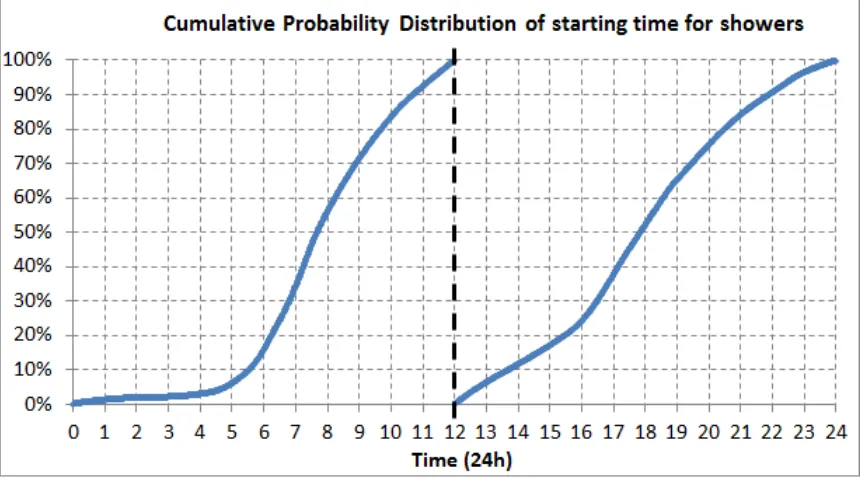
[image:44.595.109.535.150.443.2]

from 17:00 to 20:00, respectively. Figure 3.1 and Figure 3.2 show two major results of the survey. The questionnaire used in the survey is shown in APPENDIX 4.

Figure 3.1 Average number of showers versus the number of residents per household.

Figure 3.1 suggests a positive correlation between the average number of showers and the family size, in the morning and evening peaks. This correlation agrees with the common expectation that bigger families take more showers than smaller families. The unexpected drop in the average number of morning showers in households with six or more residents is most likely due to the relatively small sample size of this category of households, which is just 2.3% of the total number of households surveyed.

(45)

correlation between these two parameters exists [52]. The results of the correlation test for morning and evening showers shown in Table 3.1 indicate a positive correlation exists between the average number of showers and the family size.

Table 3.1 Correlation between average number of showers and family size

Calculated

r

Degree of freedom

Significance level

Critical value of r

Correlation exists?

Morning shower 0.552 961 0.01 0.083 Yes Evening shower 0.535 961 0.01 0.083 Yes

Figure 3.2 Histogram of the average duration of showers.

As seen from Figure 3.2, the average duration of a shower can vary from 2 min to 15 min, with a great majority of showers (about 51%) lasting from 5 min to 8 min. The mean and standard deviation of shower length were 6.5 min and 3.5 min, respectively, for the 963 filtered survey data.

Among other things, the survey also gathered data on the types of hot water system used in Tasmanian households. As shown in Figure 3.3, the majority (about 85%) of Tasmanian households use an electric hot water system. However, we cannot derive clear relationships between hot water usage and other demographic data such as

(46)

employment status and household income. For example, the vast variation of shower lengths within each demographic group prevents any conclusive inference.

Since the data obtained from the telephone survey were subjective answers given over the phone, the results are used as indicative guides in our development of the hot water consumption generator.

Figure 3.3 Distribution of types of DHWS among the surveyed households.

3.1.2 Actual energy metering data

To accurately estimate domestic hot water consumption profiles, we also acquired energy metering data from households across Tasmania. The collection period (from 20th June to 20th July 2012) included the coldest period in Tasmania. These data were obtained from meters dedicated for metering electricity in water heating alone, and represented water heating energy consumption of individual households recorded in 5-minute intervals. After the filtering process to discard erroneous data, we obtained the individual energy consumption profile of 279 households in water heating alone.

We considered two types of hot water usage:

• high volume usage that lasts for more than 5 min • low volume usage that lasts for 5 min or less

Evaluation tool for demand side management of domestic hot water load