Wind forced changes and variability in the east Australian current

(1)

WIND FORCED CHANGES AND VARIABILITY IN THE

EAST AUSTRALIAN CURRENT

by

Katherine L. Hill, M.Sc, B.Sc(hons)

Submitted in fulfilment of the requirements

for the Degree of Doctor of Philosophy in Quantitative Marine Science (A joint CSIRO and UTas PhD program in Quantitative Maxine Science)

Institute of Antarctic and Southern Ocean Studies University of Tasmania

submit date: August 2009

(2)

I declare that this thesis contains no material which has been accepted for a degree or diploma by the University or any other institution, except by way of background information and duly acknowledged in the thesis, and that, to the best of my knowledge and belief, this thesis contains no material previously published or written by another person, except where due acknowledgement is made in the text of the thesis.

. . Signed.

(3)

This thesis may be made available for loan and limited copying in ac-cordance with the Copyright Act 1968

(4)

ABSTRACT

The waters off the coast of Tasmania have become gradually warmer and saltier over the past 60 years according to a coast station time series, with sea surface tem-peratures rising at a rate more than double the global average. I demonstrate that this is related to a strengthening and more southerly reach of the East Australian Current (EAC) extension. The station also shows a strong decadal timescale signal in temperature and salinity. In this thesis, I use a combination of the Maria Island time series and Tasman Box XBT sections, 50 year atmosphere and ocean state estimates, and idealised forcing experiments with a global ocean model to build a picture of how the EAC system is changing, and what is driving it. I find that changes at Maria Island are closely related to changes in the wind stress curl in the South Pacific, with Maria Island lagging the winds by 3 years. This propagation speed is too fast for 1st Mode baroclinic Rossby wave adjustment which would take 10-15 years, so a faster mechanism is needed.

The observed variability at Maria Island is part of a bigger picture of decadal vari-ability in the Southwest Pacific region. The EAC takes one of two paths at the point of separation at 32°S; it either continues down the coast as the EAC Extension, or separates and flows across the Tasman Sea to New Zealand as the Tasman Front. On decadal timescales either the Tasman Front or the EAC Extension is favoured, which form part of two gyre scale states. When the Tasman Front is favoured, a single gyre structure is seen, which mainly sits to the north of New Zealand; whereas when the EAC extension is favoured, a double gyre structure exists, with a second gyre centre east of New Zealand. Analysis of ocean reanalyses suggests that an en-hanced wind stress curl maximum in the South Pacific appears to favour the EAC extension over the Tasman Front.

(5)

(6)

ACKNOWLEDGEMENTS

My sincere thanks go to my supervisors, Dr Stephen Rintoul and Professor Richard Coleman for their unwaivering support, guidance and patience over the last few years. I will remember Steve for never turning me away when I knocked on his door, and his inspired and broad perspective on the science. Richard has always been a voice of positivity and encouragement, and gives unwaivering support to all students he is involved with, ensuring that our PhD experience runs as smoothly and trouble free as possible. I would also like to thank Dr Peter Oke and Mr Ken Ridgway for their input and guidance.

The QMS PhD program jointly funded by the University of Tasmania and CSIRO Marine and Atmospheric Research, has provided a fabulous environment for a PhD training program. Having one PhD from both sites has meant that we have the resources of two sites at our fingertips. I have been based at CSIRO for the duration of my PhD, and the support provided to students is second to none and it has been a very positive and nurturing environment to study mostly due to genuine interest and enthusiasm of scientists down the corridor. The success of the program is due to the commitment and vision of Richard Coleman with the help of Denbeigh Armstrong. I would like to thank Armin Koehl and Ben Geise for their time and support in helping me gain access to the vast resources of data which have been produced by the GECCO and SODA reanalysis programs and Russ Fiedler for his support while I embarked on a very steep learning curve in running ocean models. I would also like to thank the two anonymous reviewers for their positive and constructive comments. Special thanks go to all the staff members of CSIRO who have been involved in collecting and processing data for the Maria Island coast station timeseries over the last 60 years, and also to those who have fought for the continuation of this remark-able resource when simple monitoring programs were not fashionremark-able. Without it, analysis of decadal ocean variability in the South Pacific would have little or no ground truthing.

(7)

PAPERS WHICH FORM PART OF

THIS THESIS

A number of articles form are in the process of being published as a result of this work. While these articles have co-authors, the figures and text included in this thesis have been produced my myself.

Some of the results from chapter 3 were published as:

Hill, K.L. and S.R. Rintoul and R. Coleman and K. Ridgway (2008) Wind forced low frequency variability in the East Australian Current Geophysical Research Letters,35 doi:10.1029/2007GL0391

Some of the result from chapter 4 will be published as:

Hill, K.L. and S.R. Rintoul and K. Ridgway and P. Oke (2008) Decadal changes in the South Pacific Western Boundary Current system revealed in observations and ocean state estimates. submitted to Journal of Geophysical Research,

Some of the results from chapter 6 will be published as:

(8)

LIST OF FIGURES

1 INTRODUCTION

iv

1

1.1 Motivation 1

1.2 Maria Island Coast Station time series - evidence of change and vari-

ability 2

1.3 Evidence of ecosystem changes 3

1.4 Regional circulation 5

1.5 The East Australian Current 7

1.6 Variability and change in the South Pacific Gyre 9 1.7 Mechanisms of decadal variability in the ocean 13 1.8 The Dynamics of wind driven circulation - local verses remote forcing 15

1.9 The aims of this thesis 18

2 DATA AND METHODS

21

2.1 Observational Data 21

2.1.1 Maria Island coast station timeseries 21

2.1.2 CSIRO Atlas of Regional Seas 23

2.1.3 Tasman Box XBT data 23

2.1.4 Climate Indices 24

2.2 Reanalysis Data 25

2.2.1 National Center for Atmospheric Research - National Cen- tre for Environmental Prediction Atmospheric Reanalysis 1

(9)

ii

2.2.2 European Centre for Medium Wave Weather Forecasting -

European Atmospheric Reanalysis-40 (ECMWF ERA-40) . . 26

2.2.3 Comparing NCAR-NCEP-1 and ECMWF ERA-40 28

2.2.4 Simple Ocean Data Assimilation (SODA) ocean reanalysis. 29

2.2.5 German-Estimating the Climate and Circulation of the Ocean

(GECCO) ocean reanalysis

30 2.2.6 BlucLINK Reanalysis

31 2.3 Analysis methods and techniques

32 2.3.1 Use of Ocean Reanalysis Products

32 2.3.2 Calculating Transports

33 2.3.3 Filtering of Timescries

37 2.4 Summary and next steps

37 3 WIND FORCED VARIABILITY IN THE EAST AUSTRALIAN

CURRENT

40 3.1 Introduction

40 3.2 Results

41 3.2.1 Analysis of T/S variability at Maria Island Coast Station . • 41

3.2.2 Changes in the wind driven circulation of the South Pacific • 44

3.2.3 The role of changes in the South Pacific wind field 50

3.2.4 Modes of variability and the EAC

54 3.3 Discussion

55 4 DECADAL CHANGES IN THE SOUTH PACIFIC WESTERN

BOUNDARY CURRENT SYSTEM REVEALED IN

OBSERVA-TIONS AND OCEAN STATE ESTIMATES 63

4.1 Introduction and motivation

63 4.2 Results

64 4.2.1 Comparing Reanalyses Products with Maria Island Coastal

Station

64 4.2.2 Relationship between Maria Island observations, wind and

volume transport

68 4.2.3 Comparing Ocean Reanalyses with Tasman Box XBT lines 69

4.2.4 Velocity structure

74

(10)

4.2.6 Role of changes in winds in determining the strength of the

EAC extension and Tasman Front

86 4.3 Summary and Conclusions

88 5 MODELS AND FORCING EXPERIMENTS

97 5.1 Motivation for model forcing experiments

97 5.2 CSIRO Ocean Model

99 5.3 Details of Forcing experiments

108 5.3-.1 Designing forcing anomaly

108 5.3.2 Sensitivity experiments

110 5.4 Analysis of model results

112 6 MECHANISMS AND RESPONSE TIMESCALES

115 6.1 Introduction and Motivation

115 6.2 Results

116 6.2.1 Response of the South Pacific to enhanced forcing in the centre

of the basin (C5 year run)

116 6.2.2 Response of the South Pacific to enhanced forcing in the east

of the basin (E5 year run)

130 6.3 Discussion

137 7 CONCLUSIONS

146 7.1 Summary of Results

147 7.2 Synthesis of ideas: the building blocks of decadal variability in the

extratropical South Pacific

149 7.3 Limitations of this study and further avenues of investigation . . . 151

7.4 Consequences of this work

154

(11)

LIST OF FIGURES

1.1 A schematic of the South Pacific wind driven circulation 6 2.1 (a) Satellite SST of the Tasman Sea for March 2001. Superimposed

are arrows showing the main regional currents. The East Australia Current (EAC), EAC Extension (EAC Ex), the Tasman Front (TF), and the East Auckland Current (EAuC); (b) Satellite SST of Tasma-nian region. Locations of the Maria Island coast station timescries and the Schouten Island Transect are marked; (c) A temperature transect offshore from Schouten Island (Cresswell 2000). The narrow shelf means that the waters in the region of the Maria coast sta-tion (50m isobath) are representative of the broader offshore

oceano-graphic conditions 22

2.2 A schematic of Tasman Box XBT sections and the currents which

cross them 24

2.3 NCEP-1 mean zonal wind stress in N/m 2 (top) and trend in N/m2 per decade (bottom). In both cases easterly is positive. 26 2.4 ERA-40 mean zonal wind stress in N/m2 (top) and trend in N/m 2

per decade (bottom). In both cases, easterly is positive. 27 2.5 South Pacific regional mean wind stress curl 20-50°S, 180-280°E for

NCEP-1 (green) and ERA-40 (pink) 29

2.6 A schematic of the Island rule. To calculate the Island rule for a particular island, winds are integrated in a closed path starting in the eastern boundary of the basin at the latitude of the northern limit of the island, across the basin, around the west coast of the island, back across the basin, and back up the eastern boundary of the basin. We define the Island rule transport through the Tasman Sea as the difference between the Island rule value for New Zealand, and the Island rule for Australia. 34 2.7 A schematic of Tasman box XBT sections and the gridstep

approxi-mation used to calculate transports from GECCO. 35

(12)

LIST OF FIGURES

2.8 Comparing rotation and stairstep methods of calculating transports across diagonal sections PX06 Auckland to Fiji (top), PX30 Brisbane to Fiji (middle)- and PX34 Sydney to Wellington (bottom) 36 2.9 Maria Island coast station SST power spectrum for unfiltered (top)

and 5 year low pass filtered (bottom) timeseries. Black line indicates the 'cone of influence', outside which, edge effects become important (Torrence Sz Compo, 1998) 38 3.1 (a) Monthly SST anomaly timescries at Maria Island Coast Station

(red) 5 year low pass filtered (black)(b) Monthly surface salinity anomaly at Maria Island coast station (blue) and 5 year low pass

filtered (black) 42

3.2 Comparing monthly sea surface temperature at Maria during (a) summer (January-March) and (b) winter (July-September) 43 3.3 Comparing monthly sea surface salinity at Maria during (a) summer

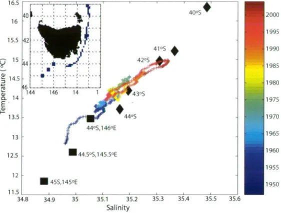
(January-March) and (b) winter (July-September) 43 3.4 The multi-coloured line is the time evolving low pass filtered surface

temperature and salinity data from Maria Island coast station (50m isobath). The diamonds represent the mean surface T/S relationship along the continental slope between the 500 and 1500m isobaths from the coastal CARS atlas (blue areas on map), +1-0.5 degrees from specified latitudes. The squares represent the colder/fresher surface climatological temperature and salinity endpoint from the CARS At-las, at the specified latitudes and longitudes (blue squares on map) south and west of Maria. 45 3.5 NCEP south Pacific zonal wind stress (eastward) for (a)1950s, (b)

3.6 NCEP mean wind stress curl for the (a) 1950s (b)1990's (c)1990s minus 1950s (*10 6 N/m3 ) in (a) and (b), the black line denotes the zero wind stress curl line. In (c), the solid line is the zero wind stress curl line for 1950s and the dashed line is the zero wind stress curl line

for the 1990s 48 3.7 The streamfunction in the South Pacific calculated from NCEP-1

wind stress and Island Rule for the a) 1950's and b) 1990's. . . . . 49 3.8 Low pass filtered (a) sea surface temperature at Maria (b) surface

salinity at Maria (c) South Pacific regional mean wind stress curl (20- 50°S, 180-280°E) from NCEP(d)net transport through the Tasman Sea calculated from NCEP and using Island rule 51 3.9 Low pass filtered (a) sea surface temperature at Maria (b) surface

salinity at Maria (c) South Pacific regional mean wind stress curl (20- 50°S, 180-280°E) from NCEP (Green) and ERA-40 (Purple) (d)net transport through the Tasman Sea from NCEP (Green) and ERA-40

(13)

LIST OF FIGURES vi

3.10 Spatial pattern of the 3 year lagged cross correlation between surface temperature at Maria and wind stress curl. Contours are time (years) required for long baroclinic Rossby waves to reach the East coast of

Australia. 54 3.11 Comparing the Maria Island SST anomaly timeseries with the

South-ern Oscillation Index (SOI). Both timeseries have been low pass fil-tered with a 5yr running mean 55 3.12 Comparing the wavelet spectra of Maria and the SOI. Black line

indicates the 'cone of influence' outside which, edge effects become important (Torrence & Compo, 1998) 56 4.1 Temperature/Salinity plots for (a) Maria (b) SODA at Maria and (c)

ECCO at Maria 66

4.2 Timeseries of (a) SST at the location of Maria, (b) Salinity at loca-tion of Maria (c) ERA-40 South Pacific regional mean wind stress curl (180-280°E, 20-50°S) and (d) SODA net southward transport through the Tasman Sea (e) SST at the location of Maria, (f) salinity at location of Maria, (g) GECCO Optimised NCEP South Pacific re-gional mean wind stress curl (180-280°E, 20-50°S) and (h) GECCO transport through the Tasman Sea 67 4.3 Temperature along PX34 from (a)XBT data, (b) BRAN (c) SODA

and (d) GECCO for overlapping years (1993-2001). Models are sam-pled during months when the XBT section was occupied. 71 4.4 Transports into the Tasman box from reanalysis data (a) PX06

Auck-land to Fiji (b) PX30 Brisbane to Fiji (c) PX34 Sydney to Wellington (positive = into the box) 73 4.5 Mean velocity across PX06 1993-2001 for (a) GECCO (b) SODA (c)

BRAN. Positive values represent flow into the Tasman Box (westward) 76 4.6 Cumulative westward transport across PX06 and north of PX06 across

180°E for GECCO, SODA, BRAN and combined XBT/Altimeter

1993-2001 77 4.7 Cumulative westward transport profiles (a)minimum (1994) and

max-imum (1962) years of transport across PX06 for SODA and (b) mini-mum (1962) and maximini-mum (2000) years of transport across PX06 for

GECCO. 79 4.8 (a) Transports for the Tasman Front and EAC Extension calculated

using a combined altimeter/XBT method (b) detrended 81 4.9 (a) Transports for the Tasman Front and EAC Extension calculated

from BRAN (b) detrended transports. 83

4.10 Transports for the Tasman Front and the EAC Extension calculated

(14)

LIST OF FIGURES

vii

4.11 Transports for the Tasman Front and the EAC Extension calculated

from (a) GECCO and (b) GECCO detrended

85 4.12 GECCO annual mean streamfunctions for (a) 1988 (Stronger EAC

Extension, weaker Tasman Front) (b) 1994 (Weaker EAC Extension,

stronger Tasman Front). Contours every 55v. 87

4.13 GECCO (a) South Pacific zonal mean wind stress curl (180-280°E)

(b) EAC Extension and Tasman Front transport

89 4.14 OFES Sea level anomaly in the Tasman Sea averaged over 38.5-45°S,

150-170°E (redrawn from Sasaki et al., 2008) (upper pannel) and Net

southward transport through the Tasman Sea from GECCO (lower

panel)

92 5.1 ERA-40 mean January zonal wind stress (N/m

2 )

100 5.2 ERA-40 mean January wind stress curl (N/m3

).

101 5.3 Bathymetry of the South Pacific (a) at model (1.875° longitude x

0.94° latitude) grid spacing. Depths in metres. (b)with major

bathy-metric features labeled. Black shaded area is above sea level,grey

shaded area is above 2000m, and grey line marks the 3500m depth

contour. 102

5.4 Temperature section across the Pacific at (a) 25°S (b) 30°S (c) 35°S

for the CARS climatology (left) and model (right) in °C 104

5.5 Temperature section across the Pacific at (a) 190°E (b) 220°E (c)

260°E for the CARS climatology (left) and model (right) in °C . . . 105

5.6 Mean South Pacific streamfunction in Sverdrups from control run (Sv)106

5.7 Mean annual cycle of net northward transport through the Tasman

Sea in Sverdrups

107 5.8 Mean annual cycle of Tasman Front transport (westward) in Sverdrups.107

5.9 Mask multipled with first year of zonal wind stress in eastern

pertur-bation run

109 5.10 ERA-40 mean January zonal wind stress with eastern perturbation

applied (N/m

2 ).

109 5.11 ERA-40 mean January zonal wind stress curl with eastern perturba-

tion applied (N/m3

)

110 5.12 Latitude/time plot of depth integrated transport across 178E

(east-ward transport north of New Zealand)in Sverdrups. This was used

to define the northern boundary of the Tasman Front as 30.5°S.. . . 114

(15)

LIST OF FIGURES

viii

6.2 Snapshots of SSH anomaly from the C5 year run (metres) at periods

after the initiation of enhanced wind forcing in the central South

Pacific. Black line represents the 3500m bathymetric contour 119

6.3 A longitude/time plot of SSH anomaly (metres) for C5 year forcing

experiment along 28°S (above) and bathymetry along 28°S 121

6.4 A longitude/time plot of SSH anomaly (metres) for C5 year forcing

experiment along 40°S

122 6.5 A longitude/time plot of SSH anomaly (metres) for C5 year forcing

experiment across 40°S

123 6.6 A schematic of the rapid mechanism by which changes in the winds in

the South Pacific can be communicated to the East Australia Current. 124

6.7 Net northward transport through the Tasman Sea for Control run

and C5 run (Sv)

126 6.8 Transport anomaly (C5 run minus control run) for EAC Extension

and Tasman Front (Sv)

127 6.9 Snapshots of SSH anomaly (in metres) for the E5 run from 1-9 days

after the initiation of enhanced wind forcing in the eastern South

Pacific. The black line represents the 3500m bathymetric contour. . 131

6.10 A longitude/time plot of SSH anomaly (metres) for E5 year forcing

experiment

132 6.11 Snapshots of SSH anomaly (metres) for the E5 year run after the

initiation of enhanced wind forcing in the eastern South Pacific. The

Black line represents the 3500m bathymetric contour. 134

6.12 Net northward transport (Sv) through the Tasman Sea for Control

run and E5 year run

135 6.13 Transport anomaly (E5 year run minus control run) for EAC Exten-

(16)

CHAPTER 1 INTRODUCTION

1.1 Motivation

A long term record from Maria Island coast station shows that the waters off the east coast of Tasmania have become warmer over the last 60 years (Ridgway, 2007). The Maria Island record also shows significant decadal variability in both temperature and salinity. Both temperature and salinity increase over this time period, especially in the summer, consistent with a strengthening and poleward extension of the East Australian Current (EAC) (Ridgway, 2007). However, the dynamics driving such a change have not been explained. Changes have also been observed in species distributions over this time period, with many species previously restricted to the coast of the Australian mainland extending their ranges southward off the coast of Tasmania (Edgar, 2000; Thresher et al., 2003; Poloczanska et al., 2007; Johnson et al., 2005; Ling, 2008; Ling et al., 2008). This is likely to have a significant impact on the Tasmanian fisheries, a major contributor to Tasmania's economy.

(17)

1.2. MARIA ISLAND COAST STATION TIME SERIES - EVIDENCE OF

CHANGE AND VARIABILITY 2

1.2 Maria Island Coast Station time series - evidence

of change and variability

(18)

1.3. EVIDENCE OF ECOSYSTEM CHANGES 3

In addition to such distinct seasonal variability, Ridgway (2007) also identified trends in temperature and salinity. The region has become both warmer and saltier, with mean trends of 2.28°C and 0.36 psu per century between 1944 and 2002, com-pared to global average estimates of sea surface temperature change of 0.09-0.14°C ±0.04°C per decade since 1960 (0.9-1.4°C per century) (Casey & Cornillion, 2001) and 0.6±0.2°C per century since 1900 (Smith

&

Reynolds, 2004). Ridgway (2007) inferred that these trends are not forced by radiative heating but are caused by an increase in the strength of the East Australia Current bringing more warm salty water south, particularly in the summer months.

1.3 Evidence of ecosystem changes

Very few comprehensive studies of relationships between variability in climate and marine ecosystems can be found, particularly in the Southern Hemisphere. Harris et al. (1987, 1988) focused on the Tasman Sea, and were the first to correlate vari-ability in climate with the success of major fisheries (Harris et al., 1988), and the composition of phytoplankton blooms in the region (Harris et al., 1987).

(19)

1.3. EVIDENCE OF ECOSYSTEM CHANGES 4

ton blooms off Tasmania has seen an increasing proportion of tropical species, such as Gefyrocapsa oceanica over the native Emiliana huxlei. Red tides, Noctiluca scin-tillans, have also appeared in Bass Strait and along the Tasmanian coastline since

2001, similar to large scale blooms seen off the coast of New South Wales in 1997 (Lyne et al., 2005). This suggests a southward range extension of species across a broad range of taxa, which broadly correlates with a southward shift in the East Australian current, bringing warm waters further south (Lyne et al., 2005). How-ever, the precise relationships have not been explored, i.e., whether a shift is due to the southward increased advection of larvae/plankton, or due to the expansion of habitat of subtropical species due limited by their viable temperature range. Further work by Poloczanska et al. (2007) produced a comprehensive study on the impacts of climate change on Australian marine life, from model results and the reviewed literature. In particular, they identified regions most at risk from the effects of climate change. The South East Australian region was defined as one of the regions most at risk from climate change, for a combination of reasons. First, it is dubbed a "Climate Hotspot", as the strengthening of the EAC is expected to continue, bringing warmer water further south. Second, it is a biogeographic transition zone, sitting between subtropical and subantarctic zones, so the region is sensitive to large scale climate shifts. Third, the South East Australian region is the most heavily populated of Australia's coastlines, so most stressed by fishing pressure (Hobday Sz Hartmann, 2006). The region was identified as particularly at risk, due to its high level of endemism. Polaczanska et al documented impacts of changing temperature and nutrient regimes on a broad spectrum of ecosystems. It was acknowledged that while impacts on individual species are relatively easy to predict, the response at the ecosystem level is much more complex.

(20)

1.4. REGIONAL CIRCULATION 5

along the coast of Tasmania has been discussed in more detail by Ling (2008) and Ling et al. (2008). It was found that a combination of larval advection and tem-perature controls determine the distribution of the sea urchins, and since the 1960's when urchins were first identified in Tasmanian waters, a transition has been seen from colonisation through larval advection, to a self sustaining community which is able to reproduce in situ (Ling et al., 2008). This is due to an increase in water temperature during August, which is generally when the water temperatures reach a minimum. August coincides with a critical period in the development of urchin larvae, which develop poorly in water temperatures below 12°C. August tempera-tures above 12°C are becoming increasingly common. The impact of this relatively new addition to the ecosystem is considerable. The macroalgal beds are grazed com-pletely, forming regions known as "barrens". The faunal community of these regions is found to be "overwhelmingly impoverished" relative to the macroalgal beds, with only 72 taxa found in barren regions, compared to 221 within intact macroalgal beds (Ling, 2008). Moreover, these macroalgal beds are the prime habitat for abalone and rock lobster, both of which are multi-million dollar fishery industries. The only effective predator of the urchins are rock lobsters much larger than the minimum catch size, which are very rare outside marine reserves. Ling (2008) highlighted the southward expansion of sea urchins as an example where changes in ocean currents can lead to disproportionately large impacts where key species with the ability to modify a habit either change or extend their range. It is also an example of the combined impacts of fishing and climate variability.

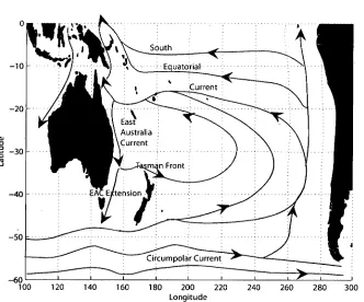
1.4 Regional circulation

(21)

240 260 280 300 160 180 200 220

Longitude East

Australia Current

Circumpolar Current

100 120 140

[image:21.555.117.449.109.385.2]

1.4. REGIONAL CIRCULATION 6

Figure 1.1: A schematic of the South Pacific wind driven circulation

(22)

1.5. THE EAST AUSTRALIAN CURRENT 7

1.5 The East Australian Current

The EAC shows some unique features when compared to other western boundary currents. Firstly, the EAC is weaker than its counterparts, with mean southward transport estimates of 22 Sv at 30°S (Mata et al., 2000) and 27 Sv at 28°S (Ridgway & Godfrey, 1994). A countercurrent runs offshore of the EAC, which is about 17 Sv of northward flow. This gives a net southward transport of 9.5 Sv (Ridgway

&

Godfrey, 1994, 1997). These transport estimates for the EAC are compared to estimates of 43 Sv - 85 Sv for the Agulhas Current (Matano et al., 2002). Moreover, it is an eddy rich current (Boland & Hamon, 1970; Boland

&

Church, 1981), so much so, that it is arguable whether it is a single current, as the baroclinic eddy mass transport is several times that of the mean flow. A more recent study, assess-ing the seasonal cycle of the EAC, suggests larger southward transports and that the seasonal amplitude is also large compared to the mean flow, with a minimum observed southward flow of 27.4 Sv in winter, and a maximum of 36.3 Sv in summer (Ridgway & Godfrey, 1997). The net transport of the EAC (including the northward countercurrent is 9.5 Sv, with a seasonal amplitude of 6 Sv. Compare this to the Florida Current at 26°S, which has a seasonal amplitude of 3 Sv with a background flow of 30 Sv (Schott et al., 1988).

A number of theories have been put forward in the literature to explain the dynam-ics and position of the separation point of the EAC from the coast of Australia and formation of the Tasman Front. Three main theories exist. Firstly, the coastline cur-vature and bathymetry around Sugarloaf Point, situated at 32.26°S (Godfrey et al., 1980); secondly, the structure of gyre-scale wind stress curl (Tilburg et al., 2001) and lastly, the blocking of westward propagating Rossby waves by New Zealand (Nilsson

&

Cresswell, 1980).

(23)

1.5. THE EAST AUSTRALIAN CURRENT 8

vary by up to 150km (Ridgway & Dunn, 2003) which means that coastline curvature and Rossby wave blocking by New Zealand are unlikely to provide the complete explanation. Bostock et al. (2006) analysed model data and foraminifera oxygen isotope ratios to infer that the latitude of the separation zone has varied since the last glacial maximum. During the last glacial maximum, the separation zone was further north between 23 and 26°S, compared to its current position around 32°S. Bostock et al suggest that the southward shift was caused by a significant change in the wind stress curl since the last glacial maximum, seemingly corroborating Tilburg et al's hypothesis. The mechanism of separation is likely to influence how the Tasman Front and the EAC extension respond to large scale wind changes and variability.

(24)

1.6. VARIABILITY AND CHANGE IN THE SOUTH PACIFIC GYRE 9

scale wind stress curl may determine the dynamics of the EAC separation and in particular the relative strength of the EAC and Tasman Front. However, the precise relationship between wind stress curl and the nature of the separation of the EAC and associated frontal systems is not fully understood.

1.6 Variability and change in the South Pacific Gyre

The observed long term trend at Maria Island, documented by Ridgway (2007), forms part of a bigger picture of observed changes in the South Pacific region. Harris et al. (1988) identified correlations between large-scale climate variability and a number of fisheries and ecosystem variables in the Tasmanian waters. They identified the number of days with strong westerly winds as the primary forcing factor, which in turn was linked to large scale climate factors, such

as

El Nino. Thresher et al. (2004) suggested that cooling at 1000m over the last three centuries, inferred from deep water coral proxies south of Tasmania, reflected an increase in the poleward flow of the EAC along the Tasmanian coast, which was in turn driven by a poleward shift of the westerly wind (Thresher, 2002; Harris et al., 1988; Oke

& England, 2004). Roemmich et al. (2007) presented evidence of a spin up of the

(25)

Mk3 climate model runs showed that an increase/shift south of the wind stress curl can cause an intensification/shift south of the EAC (Cai et al., 2005). Cai (2006) compared the NCEP winds from the 1950s to the 1990's which show a clear increase in the wind stress curl in response to a marked increase in zonal westerly winds. The Sverdrup-Island Rule solution (Godfrey, 1989) suggests a strengthened South Pacific gyre, and EAC transport increases of about 6-8 Sverdrups over 50 years, although these figures have not been compared to the observed volume flow (Cai, 2006). Climate change simulations also suggest that this trend towards a stronger gyre and a stronger EAC will continue in the future due to climate change (Cai et al., 2005). EAC transports are predicted to increase by 5-10 Sv for the mean of years 2055-2085. The change in the EAC is expected to be greater than the western boundary currents of the other subtropical gyres as the southern tip of the land boundary extends into the the zonal strip of strongest curl changes. This generates a warming rate in the Tasman sea that is the largest observed in the Southern Hemisphere in these model runs (Cai et al., 2005).

(26)

correlations on decadal timescales (Roemmich et al., 2007).

(27)

explored variability in the subtropical gyre using high resolution XBT data from the Fiji to Hawaii (PX09) and Auckland to Fiji (PX06) lines from 1987-1994. They associated interannual variability with ENSO, suggesting that relatively weak gyre scale transport is related to the La Nina event of 1988/89. After 1991, gyre scale transport was more intense. As the trade winds are strengthened during a La Nina event, but the net effect is a weaker gyre, this would suggest that it is the subtropical westerlies which have a stronger influence on the wind stress curl field and hence the strength of the South Pacific gyre.

The inverse relationship between the trades and the westerlies was also articulated by Harris et al. (1988), who linked the position of the westerly wind belt with the position of the continental high pressure over Australia and hence ENSO (as the Southern Oscillation Index is defined by the Darwin-Tahiti pressure gradient). Harris et al. (1988) also identified a clear cyclical pattern in these zonal westerly winds with a mean periodicity of 11 years. Harris et al. (1988) suggested that strong westerlies observed during El Nino events would drive colder, nutrient rich sub-antarctic waters up the east coast of Tasmania in summer. This is likely to reduce both temperature and salinity at Maria Island. Observational evidence from hydrographic and XBT data however, suggests that ENSO has a negligible influence in the EAC region. Hsieh & Hamon (1991) explored ENSO signals in using Empirical

(28)

1.7. MECHANISMS OF DECADAL VARIABILITY IN THE OCEAN 13

also that there was little evidence of in-phase ENSO related changes found south of about 10°S. Further work is needed to examine the relationship between decadal ENSO, the trade winds and subtropical westerly winds, and the net effect on the wind stress curl and hence the South Pacific gyre strength.

1.7 Mechanisms of decadal variability in the ocean

Timescales of variability in the ocean are generally thought to be dictated by at-mospheric and oceanic teleconnections. As discussed above, ENSO-like decadal variability in the Pacific is known by a number of names (see further discussion in section 2.1.4). Essentially the signal in question is the same. In addition to the timescale, the difference between interannual ENSO variability and low frequency decadal ENSO variability is seen in the spatial pattern. Power et al. (1999) describe the Interdecadal Pacific Oscillation as a ENSO type spatial structure with a broader tropical signature, and a stronger extratropical signature.

(29)

1.7. MECHANISMS OF DECADAL VARIABILITY IN THE OCEAN 14

Pacific subtropical gyre and hence variations in the strength of the Kuroshio Ex-tension. However, Schneider et al. (2002) suggests it is stochastic variability in the Aleutian Low which changes the Ekman pumping over the North Pacific, which excites Rossby waves; and it is this Rossby wave propagation which dictates the timescale of variability. No evidence is found for a mid-latitude ocean-atmosphere negative feedback loop.

(30)

1.8. THE DYNAMICS OF WIND DRIVEN CIRCULATION - LOCAL VERSES

REMOTE FORCING 15

also needs to be articulated.

1.8 The Dynamics of wind driven circulation - local

verses remote forcing

(31)

1.8. THE DYNAMICS OF WIND DRIVEN CIRCULATION - LOCAL VERSES REMOTE FORCING 16

years between changes in scatterometer-derived wind stress curl in the South Pacific and the ocean's response in altimetric SSH. Roemmich et al. (2007) also noted a lag between the peak in the wind forcing over the subtropical South Pacific, and the peak in the response of the ocean, in terms of the strength of the subtropical gyre circulation, of about 4-5 years. Schneider 8z Miller (2001) used wind stress data and a Rossby wave model to demonstrate that variations in wind stress in the central North Pacific manifest as winter SST anomalies in the Kuroshio-Oyashio extension with a 3 year lag. These studies suggest that a faster mechanism than first mode baroclinic Rossby waves is responsible for the observed time lag between wind forcing and the response of western boundary currents. However, both Qiu & Chen (2006) and Schneider 86 Miller (2001) conclude that the baroclinic Rossby wave dynamics provide the basis for the observed SSH variability in the subtropical gyres of the Pacific on interannual to decadal timescales. This conclusion relies on the integrating nature of Rossby waves along their pathway. As Qiu & Chen (2006) force their linear model with basin scale wind anomalies, it was not possible to iso-late the region(s) of forcing which was critical to creating the observed variability in SSH.

(32)

1.8. THE DYNAMICS OF WIND DRIVEN CIRCULATION - LOCAL VERSES REMOTE FORCING 17

primarily barotropic (Veronis & Stommel, 1956; Gill

&

Niiler, 1973). Reid (1986) suggested that the barotropic component is small in the subtropical gyre, although Fu & Davidson (1995) found a relatively large response to wind forcing in the south-east Pacific, south of 30°S. North of 29°S, annual SSH variability is influenced by local isopycnal response to Ekman pumping (Roemmich & Cornuelle, 1990; Morris et al., 1996). However, annual variations in the thermocline do not dominate south of 29°S (Roemmich & Cornuelle, 1990).

More recently, model experiments have been used to explore the role of topography in modifying planetary wave propagation, and the consequences for ocean adjust-ment. Tanaka

&

Ikeda (2004) explored variability in the Kuroshio region using a regional model with simple ridge topography and an idealised wind stress anomaly. They investigated the interaction of barotropic and baroclinic Rossby waves at dif-ferent timescales across the ocean ridges and found that on interannual timescales and longer, barotropic waves have very little success in crossing the ridges. Baro-clinic waves tend to be transmitted across the ridges, having a net mass transport, and therefore modifying the Kuroshio Current. However, on seasonal and shorter timescales, baroclinic waves forced directly by the winds dissipate quickly. How-ever, barotropic wave energy appears to be effectively transmitted to the west of the ridge, by conversion to baroclinic modes on the ridge within a few years of the wind perturbation. Tanaka & Ikeda (2004) conclude that the balance between baroclinic and barotropic modes is dependant on the frequency of forcing and their modification across the ridge appears to be related to the interaction between the wavelength of forcing and ridge width.

(33)

1.9. THE AIMS OF THIS THESIS 18

the cast coast of the island. The direction of circulation around the island is set up by a coastal Kelvin wave, which propagates around the coast, and the circulation is completed by long Rossby waves, which are initiated on the west coast of the island. Sasaki et al. (2008) suggested that this theory could be applied to the South Pacific, where sea level variability in the Tasman Sea can be explained by changes in the South Pacific wind stress curl field and the signal is then communicated around the New Zealand coast.

The results of Tanaka igz Ikeda (2004) and Liu et al. (1999) suggest that wind forcing could initiate variability on the western boundary with a lag of a few years, by the conversion between barotropic and baroclinic modes through interaction with islands or ocean ridges.

1.9 The aims of this thesis

We can say with certainty that the waters off Tasmania have been getting warmer and saltier since 1944. The trend in temperature is double the global average sea surface temperature change over the same time period, and is certainly related to a strengthening of the EAC. There is also distinct decadal timescale variability in the strength of the EAC, and hence temperature and salinity. There is mounting evidence that such changes and variability are causing changes in the distribution of species across a broad range of taxa, resulting in significant ecosystem changes. One particular example is the establishment of spiny sea urchins Centrostephanus rogersii in Tasmanian waters, and the related destructive grazing of giant kelp forests. This thesis explores the causes of observed changes and variability in the EAC system. In particular, I focus on three specific questions:

(34)

South Pacific wind driven gyre, and observed changes in the South Tasman Sea?

2. How is observed EAC variability related to the regional current system? Can we build a picture of regional decadal variability using new 50-year ocean reanalysis products?

3. What are the mechanisms by which the ocean communicates remote south Pacific wind forcing to changes in the EAC, and how is this achieved within a few years, when the theoretical first mode baroclinic response would take 10-20 years?

(35)

particular, I identify that the transport of the EAC Extension and the Tasman Front are strongly anticorrelated, and this is representative of changes in the circulation of the gyre driven by changes in South Pacific wind stress curl. The data and methods for this study are found in chapter 2, and the results in chapter 4.

(36)

CHAPTER 2 DATA AND METHODS

In this chapter, I outline the datasets and methods of analysis used in chapters 3 and 4.

2.1 Observational Data

2.1.1 Maria Island coast station timeseries

The Maria Island Time Series (Maria) station is situated off the southeast coast of Tasmania at 42.6°S, 148.23°E. It is the longest high quality time series station in the Southern Hemisphere, running from 1944 to the present day. The station is located at the 50 m isobath, approximately 5 km from the edge of the narrow continental shelf. Monthly temperature, salinity and nutrient measurements are taken from the surface to 50 metres, at 10 metre intervals. While most of the EAC separates near 30°S forming the Tasman Front, the remainder of the current continues southward to form the EAC Extension (Creswell, 2000) (Figure 1.1). The ribbon of warm water carried south by the EAC Extension lies over the upper continental slope, just offshore of Maria Island (Figures 2.1b and c). Ridgway (2007) used satellite measurements of surface temperature to confirm that the Maria temperature record represented the temperature of the EAC Extension and was correlated with surface temperature over a broader region.

(37)

2.1. OBSERVATIONAL DATA 22

-25

-35

-J

-40

-45

140 150 160 170

Longitude

°

C

/

8

4

16

4

1

0

2

12 180

-44 4aiii 11 42

146 148 150 152

°C

[image:37.556.183.376.121.629.2]

Longitude

Figure 2.1: (a) Satellite SST of the Tasman Sea for March 2001. Superimposed

(38)

2.1.2 CSIRO Atlas of Regional Seas

The CSIRO Atlas of Regional Seas (CARS 2006) and the CARS coastal (Coast8

2006) datasets were used to compare Maria data with the regional background

cli-matology temperature and salinity (Ridgway et al., 2002; Dunn & Ridgway, 2002).

CARS is a digital atlas of seasonal ocean water properties produced from

hydrog-raphy data taken from the BlueLINK BOA (BLUElink Ocean Archive), which in

turn is based on a number of datasets including the World Ocean Database 2001

(WOD01), the World Ocean Circulation Experiment World Hydrographic Program

1 (WOCE-WHP1), CSIRO data holdings, and the Argo float network. Stations such

as Maria Island coast station are included in the CARS analysis. CARS initially

focused on the seas around Australia, but now extends to the Southern Hemisphere

and tropics. Temperature, salinity, oxygen, nitrate, silicate and phosphate are all

mapped onto 79 depth levels, with 0.5x0.5 degree resolution in the region 0-360°E,

70°S to 26°N (10°N in the Atlantic). Coast8 is a high resolution version of CARS, at

1/8° resolution for a polygon encompassing the Australian coastal and shelf waters

defined within the region 110-155°E, 18-50°S.

2.1.3 Tasman Box XBT data

The Tasman Box consists of 3 XBT lines, which form a closed box in the South

West Pacific (Roemmich et al., 2005). These lines are PX06 (Auckland to Fiji),

PX30 (Fiji to Brisbane) and PX34 (Sydney to Wellington) (Figure 2.2). This region

encompasses the EAC, the South Equatorial Current and the Tasman Front. These

lines are occupied quarterly, and XBT's are dropped every 40 km in the open ocean,

and every 15-20km inshore. The Fiji to Brisbane and Sydney to Wellington lines

have been running since 1991, and the Auckland to Fiji line has been established

(39)

160 165 Longitude

170 175 180

Figure 2.2: A schematic of Tasman Box XBT sections and the currents which cross them

geostrophic transports into and out of the Tasman Box (for full details see Ridgway,

2008). Ekman transport was incorporated to give an estimate of total transport by

calculating the Ekman pumping along the XBT sections from ERA-40 wind stress

data.

2.1.4 Climate Indices

The Southern Oscillation Index (SOI) and the Southern Annular Mode (SAM)

In-dex were low pass filtered with a 5 year running mean to determine their relationship

with the observed low frequency variability in the Maria coast station timeseries.

The Southern Oscillation Index is calculated from the Darwin-Tahiti sea level

pres-sure difference (Trenberth, 1984). A number of papers have discussed low frequency

variability in the Pacific region, which goes by a number of names and is calculated

in a variety of ways. These include the Pacific Decadal Oscillation (PDO) (the first

EOF of North Pacific and tropical SST (Mantua et al., 1997)), the Interdecadal

Pacific Oscillation (IPO) (first near-global EOF of SST (Folland et al.,

1998;

Power et al., 1999)) and Decadal ENSO (calculated by projecting the spatial pattern of

(40)

2.2. REANALYSIS DATA 25

(20°S-20°N, 120°E-70°W) onto the unfiltered SSH in the same region (Sasaki et al., 2008)). However calculated, the low frequency variability in the ENSO system dom-inates and Power et al. (1999) demonstrated that a low pass filtered SOT, the PDO and the IPO are highly correlated (r=>0.9) since 1945 (prior to this, differences are likely due to instrument error). Therefore, for simplicity, a 5 year low pass filtered SOT is used to represent the low frequency variability in the ENSO system, and we will call this signal decadal ENSO. The SAM index was obtained from the 1st EOF of Southern Hemisphere NCEP-2 (1979-present) Sea Level Pressure. Prior to 1979, there is not sufficient data in the Southern Hemisphere to give a reliable SAM index (see discussion of trends in NCEP-1 reanalysis in section 2.2.2).

2.2 Reanalysis Data

2.2.1 National Center for Atmospheric Research - National Cen-tre for Environmental Prediction Atmospheric Reanalysis 1 (NCAR/NCEP-1)

(41)

150 200

Longitude 250 300

100 350

50

-0.05 -0.1

015

02

0.02

0.015

0.01

0.005

0

-0005

- 001

- 0.015

40

20 -o

-20

-40

- 60

-ao

10.2

0.15

0.1

0.05

50 100 150 200 250 300 350

[image:41.556.172.389.121.465.2]

Longitude

Figure 2.3: NCEP-1 mean zonal wind stress in N/m 2 (top) and trend in N/m2 per decade (bottom). In both cases easterly is positive.

far the dominant feature of this figure is the strong positive trend in wind stress

(0.01-0.02 N/m2 per decade) in a coherent zonal band between 50 and 70°S. This

trend is strongest in the South Indian Ocean sector. A weakening of the trade winds

in the tropical Pacific is also apparent (-0.01 N/m 2 per decade).

2.2.2

European Centre for Medium Wave Weather Forecasting -

European Atmospheric Reanalysis-40 (ECMWF ERA-40)

ECMWF ERA-40 is a 40 year global reanalysis product, running from 1957-2001,

(42)

350 0 50 100 150 200

Longitude

- 0.05

-a

1

- 0.15 - 0.2

0.02

0.015

0.01

0.005

- 0 005

- 001

- 0015

-002 100 150 200 250 300 350

Longitude

[image:42.558.173.391.120.466.2]

Figure 2.4: ERA-40 mean zonal wind stress in N/m 2 (top) and trend in N/m 2 per decade (bottom). In both cases, easterly is positive.

used. As with NCEP-1, inconsistencies have been noted related to the evolution

of the observing system, which impacts the high latitude southern hemisphere in

particular (Bromwich

&

Wang, 2008). The mean and the trend in zonal winds is

shown in Figure 2.4. A hemispheric strengthening of winds is seen centred on 60°S

albeit patchy. Maximum trend values are around 0.01-0.02 N/m 2 per decade. This

trend is strongest in the South Indian Ocean. The weakening of the trade winds is

(43)

2.2.3 Comparing NCAR-NCEP-1 and ECMWF ERA-40

NCEP-1 and ERA-40 represent two approaches to developing atmospheric reanal-yses. As discussed above, much attention in the literature has focussed on the enhanced trend in the polar vortex, found in NCEP-1 as discussed above. Analy-sis suggests that ERA-40 is more accurate during the satellite era (1980 onwards). ERA-40 is more reliant on satellite data than NCEP-1, which relies on station based data, so there are larger inconsistencies in ERA-40 prior to the satellite era (Bromwich & Fogt, 2004; Bromwich & Wang, 2008). Figures 2.3 (NCEP-1) and 2.4 (ERA-40) highlight the differences between the two models in terms of mean zonal winds and trend. Both NCEP and ERA-40 products show a positive trend in the southern hemisphere westerly winds with maximum values of around +0.02 m/s per decade (Figure 2.3 and 2.4). However, the trend in the southern hemisphere westerlies since 1960 appears to be more zonally coherent in NCEP, especially from Southern Africa to south of Australia and New Zealand, whereas the trend in ERA-40 is much more patchy. While much attention has focused on differences and inconsistencies at high latitudes, Grotjan (2008) also identified significant differ-ences in primary circulation and energetics of the two products in the equatorial region. In Figures 2.3 and 2.4, NCEP-1 also shows a more coherent weakening of the trade winds in the tropical Pacific than ERA-40.

(44)

Figure 2.5: South Pacific regional mean wind stress curl 20-50°S, 180-280°E for NCEP-1 (green) and ERA-40 (pink).

the focus of this study. While there are some shortcomings in both of these wind

product datasets, they represent the best effort in recreating the structure of the

atmosphere over the last 50 years. Results from both reanalyses will be discussed

in chapters 3 and 4.

2.2.4 Simple Ocean Data Assimilation (SODA) ocean reanalysis

SODA version 2.0.2 is a 0.5 degree ocean reanalysis product covering the 44 year

period between 1958 and 2001 forced by ERA-40 winds (Carton & Giese, 2006). The

model uses the Parallel Ocean Program (POP) model with an average resolution

of 0.25° and 0.4° in the zonal and meridional directions and has 40 vertical levels.

Fields from SODA that are used here have been mapped onto a 0.5 degree grid

using optimal interpolation. Because altimeter sea level observations represent such

a major change in the observation base, these are excluded from the reanalysis.

SODA employs a sequential data assimilation scheme that uses fields from the

nu-merical model as a background field at the update time (every 10 days). At each

(45)

by combining the background field with an array of observations. The model is ini-tialised with the analysis and integrated forward in time until the next assimilation step. Due to the sequential nature of the adjustments, the reanalysis fields do not generally conserve mass or heat.

Steric sea level rise was assessed by comparing SODA version 1.2 with 20 tide gauge station sea level records from around the world on sub-seasonal timescales (Carton et al., 2005). A positive relationship was found at all selected tide gauge stations, with an average correlation of r=0.7. This represents a substantial improvement on previous versions of the SODA reanalysis. Carton et al. (2005) also compared the SODA dynamic height with altimeter sea level, and found very good spatial agreement in the linear trends with sea level rise concentrated in the western Tropical Pacific, eastern Indian and Southern Ocean. This is promising considering that altimeter data are excluded from the reanalysis.

2.2.5 German-Estimating the Climate and Circulation of the Ocean (GECCO) ocean reanalysis

GECCO is based on the 1 degree ECCO/MIT adjoint ocean model, which is brought into consistency with satellite and in situ observations from 1952-2001 (Koehl et al., 2006). During the optimization, initial temperature and salinity conditions, as well as time dependant fluxes of momentum, heat and freshwater, are adjusted by an adjoint method in order to bring the model into agreement with observations. Back-ground forcing consists of NCEP-1 wind stress, net heat and freshwater fluxes. This approach is therefore mass and energy conserving.

(46)

in this region. The first 10 years of GECCO were excluded from this study due to issues with long term adjustment processes to the initial conditions (Kochi et al., 2006).

Comparison of GECCO with observations of the tropical Atlantic circulation sug-gests that GECCO produces the transports of the major currents well (Rabe et al., 2008). The dynamically consistent assimilation scheme doesn't introduce artificial source or sink terms into the ocean. However, it was found that unresolved processes (in particular, due to coarse model resolution) may project onto the forcing fields during the optimisation process, so winds may not be more realistic in all regions. While these wind perturbations appeared to be an effect on seasonal to interannual timescales, Rabe et al. (2008) suggest long term variability in wind stress forcing seems less perturbed in this way. GECCO has also been used to assess decadal sea level changes (Koehl

&

Stammer, 2007). Regional changes in sea level were linked predominantly with an intensified sub-tropical gyre circulation and the associated heat redistribution.

In summary, no model can perfectly represent the ocean due to unresolved processes and numerical errors. GECCO and SODA take different approaches to managing these model deficiencies. GECCO, by adjusting the surface fluxes, and SODA by having artifical sources of heat and momentum in the ocean.

2.2.6 BlueLINK Reanalysis

(47)

2.3. ANALYSIS METHODS AND TECHNIQUES 32

higher spatial resolution than SODA or GECCO. The ocean model is the Ocean Forecasting Australia Model (OFAM) which is based on version 4.0d of the GFDL Modular Ocean Model (Griffies et al., 2004) and is driven by surface fluxes from the ECMWF, including ERA-40, for its duration (until 2001) and operational forecast fields thereafter. The horizontal resolution of OFAM ranges from 1/10 0 around Australia, to 0.9° across the Indian and Pacific oceans to 2° in the North Atlantic. BRAN will be used in this study for comparisons made during the XBT era. An advantage of BRAN is that its performance has been comprehensively assessed in the region of interest (Schiller et al., 2008), by comparing the structure and transport of major boundary currents around Australia, providing new insights into the structure and dynamics of the EAC at eddy resolving scales. It was noted by Schiller et al. (2008) that the depth penetration of the EAC was greater than expected, suggesting that the EAC influence may extend through the entire water column.

2.3 Analysis methods and techniques

2.3.1 Use of Ocean Reanalysis Products

(48)

gain insight into the relationships between the main currents, but only for the last 15 years.

Instead of using direct observations to understand ocean variability, an alternative information source are ocean reanalyses. These products provide the only source of estimates of ocean state over multidecadal timescales. Thus, a combination of the GECCO and SODA 50 year ocean reanalyses, Maria, XBT sections and altimeter data are used to explain the role of changes in the South Pacific wind field in causing the decadal variability observed in the EAC system over the last 50 years.

2.3.2 Calculating Transports

Calculating streamfunction and transports from wind fields

Wind stress curl fields were calculated from both NCEP-1 and ERA-40. South Pacific streamfunctions and transports through the Tasman Sea were then calculated using the Island Rule (Godfrey, 1989) for each whole decade, and then compared. The Island Rule is an adaptation of the Sverdrup approximation, which allows for flow around islands. Wind stress curl is integrated in a path from the eastern boundary of the basin, round the back of an island to determine the wind driven flow around that island (Figure 2.6). This gives a transport value to the island, which then allows the streamfunction around the island to be contoured. Consequently, the transport through the Tasman Sea (or net EAC transport) was defined as the difference in Island Rule values for Australia and New Zealand.

Calculating Transport across diagonal sections from gridded Ocean Ve-locity

(49)

-60 L

100 120 140 160 180 200 220 240 260 280 300 Longitude

Figure 2.6: A schematic of the Island rule. To calculate the Island rule for a partic-ular island, winds are integrated in a closed path starting in the eastern boundary of the basin at the latitude of the northern limit of the island, across the basin, around the west coast of the island, back across the basin, and back up the eastern boundary of the basin. We define the Island rule transport through the Tasman Sea as the difference between the Island rule value for New Zealand, and the Island rule for Australia.

Tasman Box. As ECCO and SODA use different model grids, different approaches

to the calculations were taken. GECCO uses a C grid model which allows a "stair

step" approach to be used (see Figure 2.7) without the need for interpolation (Koehl

et al., 2006). The sum of transports in to and out of the box balanced to within

10-5 Sv, and the net transport through the Tasman Sea averages 5 Sv to the South.

SODA and BRAN use a B-grid model, and in the case of SODA, the results are then

remapped, so an approach is used whereby velocity vectors were interpolated to the

particular XBT section and then rotated so that they were perpendicular or normal

to the section (Oke et al., 2008; Carton SL Giese, 2006). Using this approach, the sum of the transports balance to within -0.9 Sv for SODA and -1.6 Sv for BRAN

in the mean. While we acknowledge that this approach may introduce some errors,

the errors were larger when a stair step method was used (mean inbalance: -4 Sv

(50)

15

- 20

-25

- 30

-35

-40

PX34

4 45

170 165 155 160

150 175 180

Figure 2.7: A schematic of Tasman box XBT sections and the gridstep approxima-tion used to calculate transports from GECCO.

Sydney to Wellington section which crosses a highly dynamic region of the EAC,

close to the separation point (see Figure 2.8). Thus, it was decided to stay true to

the XBT section and rotate the velocities. Furthermore, the imbalance appeared as

a net offset of 1.6 Sv with an RMS of 1.8 Sv. Therefore while the actual values may

be subject to an error, we have confidence in interpreting the patterns of variability.

Representation of mesoscale structure and variability along the Sydney to

Welling-ton line maybe the source of this offset. In the case of BRAN, the higher resolution

may introduce errors from small temporal scale variability, whose timescales are

un-resolved in monthly mean. In the case of SODA, the interpolation from the original

model grid to the output grid is another source of error.

To plot velocity and temperature sections, GECCO, SODA and BRAN data were

interpolated onto the XBT lines. Velocities were rotated to illustrate cross sectional

velocity. To illustrate the influence of the position of the SEC on transport across

the Auckland to Fiji line, and the extent to which the SEC is partitioned by Fiji,

velocity sections were extended north of Fiji towards the equator along 180E.

(51)

2.3. ANALYSIS METHODS AND TECHNIQUES 36

15

10

5

1996 1997 1998 1999 2000 2001 2002 2003 2004 2005

[image:51.556.101.486.213.510.2]

Time (years)

Figure 2.8: Comparing rotation and stairstep methods of calculating transports

across diagonal sections PX06 Auckland to Fiji (top), PX30 Brisbane to

Fiji

(middle)

(52)

2.4. SUMMARY AND NEXT STEPS 37

sum of transport across the southern section of the Auckland to Fiji line. The northern limit of this analysis was identified in mean rotated velocity sections where there was a coherent transition from eastward to westward velocities. We define this as 32°S for BRAN, 28°S for SODA and 27°S for GECCO (compared to 31°S for the XBT/Altimeter method). A different cut-off latitude was used for GECCO, as features, such as the Tasman Front, are smoother and broader due to the reduced resolution. As the Sydney to Wellington section crosses close to the point where a portion of the EAC separates from the coast to form the Tasman Front, the transport calculations could be contaminated by eddies if the same method was employed. Therefore, the EAC Extension transport was defined as the net southward transport through the Tasman Sea, across the Sydney to Wellington line.

2.3.3 Filtering of Timeseries

To focus on the lower frequency signals in the time series of interest, low pass filtering has been used in the form of a 5 year running mean. This has been used on all time series data to allow us to focus on decadal timescale variability. Figure 2.9 shows the wavelet spectrum for the filtered and the unfiltered Maria time series. The spectrum for the unfiltered time series shows a coherent energy signal on decadal timescales throughout the full time series, in addition to interannual energy which does not seem to fit a consistent timescale throughout the period. The wavelet spectrum of the low pass filtered time series shows that these interannual signals were effectively filtered out, while preserving most of the decadal timescale energy.

2.4 Summary and next steps

(53)

p

er

io

d (y

ears)

10° 10'

100 200 300 400

_time(years)

500 600

15

2.5

2

4.5

4

3.5

3

1.5

05

15

2.5

2

4.5

4

3.5

3

1.5

0.5

10 1

p

erio

d (y

ears)

100

100 200 300

400 500 600

time(years)

(54)

(55)

CHAPTER 3 Wind forced variability in the East

Australian Current

3.1 Introduction

In this chapter I use Maria Island coast station timeseries, and NCEP and ERA-40 reanalysis winds to make the case that changes in temperature and salinity at Maria are representative of changes in the strength or southward penetration of the EAC. I also present evidence that low frequency variability in the East Australian Current is closely related to low frequency variability in the South Pacific winds. Finally I conclude that the EAC responds to changes in the South Pacific winds faster than is possible by a first mode baroclinic Rossby wave response.

The chapter is set out as follows. First, the observed variability in temperature and salinity from Maria Island coast station time series is described. The relationship between Maria and the EAC is discussed in the context of regional climatology T/S properties in section 3.2.1. The observed changes and variability in the South Pacific wind field are then described in section 3.2.2, and in section 3.2.3, variations in wind driven circulation and net EAC Extension transport are deduced from Island Rule calculations. Section 3.2.4 focuses on the relationship between Maria Island coast station and variations in the South Pacific wind field and section 3.3 is the discussion

(56)

3.2. RESULTS 41

for this chapter.

Some of the results in this chapter have been published: Hill, K.L. and S.R. Rintoul and R. Coleman and K. Ridgway (2008) Wind forced low frequency variability in the East Australian Current Geophysical Research Letters,35 doi:10.102912007GL0391

3.2 Results

3.2.1 Analysis of T/S variability at Maria Island Coast Station

Temperature and salinity timeseries from Maria Island coast station both exhibit a strong positive trend, as well as significant decadal timescale variability (Figure 3.1). The trend in temperature and salinity from 1944-2006 is equivalent to +0.22°C and +0.03psu per decade, respectively. This rate of change is 2-3 times that of the global average ocean temperature trend (Ridgway, 2007; Smith & Reynolds, 2004; Casey & Cornillion, 2001).

On annual timescales, sea surface temperature and salinity (T/S) at Maria Island coast station show significant seasonal variability (see Figures 3.2 and 3.3), with an annual amplitude of 4.2°C and 0.05 psu respectively. This is related to the seasonal variability in the strength of the EAC, which is stronger in austral summer (defined as January to March) than winter (July to September) and brings warm salty water down the east coast of Australia (Cresswell, 2000; Ridgway, 2007). The trend in both temperature and salinity is also stronger in summer (+0.25°C and +0.05 psu per decade ) than winter (+0.15°C and +0.02 psu per decade), suggesting this is also related to changes in the strength of the EAC.

(57)

—0.4

2010

1940 1950 1960 1970 1980

time (years) 1990 2000

(b)

0.6

0.4

0.2

3.2. RESULTS 42

(a)

2.5

2

1.5

—IS

—2

—2.5

1940 1950 1960 1970 1980 1990 2000 2010

time (years)

(58)

Temp era ture ( °C) 19 18 17 16 15 14 13 1940 15 14 13 12 11 10 9 (a) (b)

1960 1970 1980

1950 1990 2000 2010

3.2. RESULTS 43

1940 1950 1960 1970 1980 1990 2000 2010 Time (years)

Figure 3.2: Comparing monthly sea surface temperature at Maria during (a) summer (January-March) and (b) winter (July-September)

(a) 35.6

35.4

a

_a

35.2

35 -

34.8

34.6 1940 (b) 35.6

35.4 0. 35.2 35 34.8 34.6

1950 1960 1970 1980 1990 2000 2010

1

1940 1950 1960 1970 1980 1990 2000 2010 Time (years)

Wind forced changes and variability in the east Australian current