A Simplified Artificial Life Model for Multiobjective Optimisation: A Preliminary Report

A Simplified Artificial Life Model for Multiobjective Optimisation:

A Preliminary Report

Adam Berry

School of Computing University of Tasmania

Private Bag 100 Hobart TAS Australia 7001

[email protected]

Peter Vamplew

Private Bag 100 Hobart TAS Australia 7001 [email protected]

Abstract- Recent research in the field of Multiobjective Optimisation (MOO) has been focused on achieving the Pareto optimal front by explicitly analysing the dominance level of individual solutions. While such approaches have produced good results for a variety of problems, they are computationally expensive due to the complexities of deriving the dominance level for each solution against the entire population. TB_MOO (Threshold Based Multiobjective Optimisation) is a new artificial life approach to MOO problems that does not analyse dominance, nor perform any agent-agent comparisons. This reduction in complexity results in a significant decrease in processing overhead. Results show that TB_MOO performs comparably, and often better, than its more complicated counter-parts with respect to distance from the Pareto optimal front, but is slightly weaker in terms of distribution and extent.

1 Introduction

Most real-world problems inherently contain multiple, frequently conflicting, objectives (Coello, 1999). While conventional genetic algorithms endeavour to solve this problem through an a priori technique, this is constrained by the need for pre-existing expert knowledge about the problem being examined. The approach adopted by multiobjective optimisers (MOOs) is to assume nothing about the problem and generate a list of viable alternatives that represent the best available trade-offs between the conflicting objectives (commonly referred to as the Pareto optimal front). Thus, multiobjective optimisers represent an excellent tool for the design phase of real-world projects, enabling the expert to examine trends in the Pareto optimal front, test possible solutions or develop an understanding of the relationship between objectives.

The practical applicability of MOOs has seen the field garner increasing attention in recent years. Given this increased research focus, the variety of approaches suggested is vast (see Coello, 2001; Coello, 1999; Van Veldhuizen and Lamont, 1998). However, the most successful evolutionary techniques (such as SPEAII [Zitzler et al., 2002a] and NSGAII [Deb et al., 2000]) feature the notion of solution dominance to guide progress towards the Pareto optimal front. While this has proven to be effective, it comes with a significant computational burden that enforces a practical limit on population size and thus reduces

the likelihood of finding complex fronts.

Consequently, this paper introduces a new approach to multiobjective optimisation that forgoes the need to calculate solution dominance and capitalises on the basic principles of artificial life (ALife). Although the combination of ALife and MOO is not unique (Socha and Kisiel-Dorohinicki, 2002; Laumanns et al., 1998), the approach adopted by TB_MOO is a significant departure from pre-existing agent-based evolutionary approaches. Moreover, the technique is designed with the explicit purpose of minimising computational overhead.

2 Definitions

2.1 Multiobjective Optimisation

The explicit goal of all MOOs, as intimated in the introduction, is developing the Pareto optimal front for a problem which has multiple objectives. A single solution is said to be Pareto optimal if it is not dominated by any other possible solution, while the Pareto optimal front is formed by the set of all non-dominated solutions. In a minimisation1 problem with n objectives, solution a dominates b if and only if:

i {1, …, n} : fi(a) fi(b)

j {1, …, n} : fj(a) < fj(b) (1)

where f is an objective function that maps a multi-variate solution to a single value (as per the definition provided by Zitzler et al., 1999).

The definition of a non-dominated solution a for a population of solutions P can thus be given as:

p P : (a dominates p) (p = a) (2) (p is not comparable with a) (3) where (2) is typically referred to as weak dominance and p is not comparable with a if it is better than a in one objective but worse in another (for a dual-objective problem).

It is important to note that, for most real-world problems, the set produced by a multiobjective optimiser will likely be an approximation of the Pareto optimal front (Zitzler et al., 2002b). Indeed, for continuous functions, a complete set would effectively require an infinite number of solutions. As such, the quality of a produced set is typically measured by analysing performance metrics that are designed to gauge how well a set represents the true Pareto optimal front.

2.2 Artificial Life Systems

The definition of artificial life is open to conjecture, primarily due to the difficulties of defining life in general. This paper adopts a minimalist approach, in which an ALife system is any environment where resources are consumed, stored and expended, and fitness is assessed endogenously. Solutions in ALife systems are encapsulated as agents, who interact within the environment. Thus, the term artificial life is invoked, in this case, to highlight the novelties of an approach that is divergent from the per-turn, artificial evolution evident in techniques such as genetic algorithms. In ALife systems, a turn represents an opportunity to gather resources – the success of which is not just dependent on the adaptiveness of the agent, but also the peculiarities of the environment. An agent breeds only when it is fit enough to do so and only if it is fortunate enough and resourceful enough to survive that long. In essence, artificial life systems are inherently noisy – but that noise should result in a wide diversity of agents, without a significant cost to elitism.

3 Existing Evolutionary Approaches

The range of evolutionary approaches designed to optimise multiobjective problems is vast and it is certainly not the aim of this paper to analyse the field as a whole. Instead, the most prevalent general categories of recent research will be briefly presented, with examples and critiques provided. For a more extensive review, the reader is again directed towards the excellent summary pieces by Coello (1999 and 2001) and Veldhuizen and Lamont (1998).

3.1 Explicit Use of Dominance

While the notion of solution dominance as a fitness measure has been part of multiobjective literature since the concept was first suggested by Goldberg (Goldberg, 1989;Goldberg and Richardson, 1987), it is still the focus of considerable research and such an approach seems “to be the most popular in the field” (Zitzler et al., 1999). The general principle of explicit dominance use (or Pareto ranking, as it is also known) is straightforward – in an evolutionary system, fitness is assigned according to the level of dominance achieved for a given solution. If the solution is non-dominated, then it receives a high score and is thus more likely to breed. If the solution is dominated by large numbers of the population, then it receives a low ranking and is less likely to propagate.

The specific mapping from dominance to fitness varies, but the general hypothesis remains the same: that maintaining and evolving a set of highly dominant solutions can achieve a good approximation of the Pareto optimal front. Experimental results have shown this hypothesis to be largely true. For instance, a comparative study by Zitzler et al. (1999) showed that a range of dominance based approaches, such as SPEA (Zitzler and Thiele, 1998) and NSGA (Srinivas and Deb, 1994), performed well on a variety of test problems designed to reflect the different classes of multiobjective problems.

While the quality of approximations produced by Pareto ranking methods is generally impressive, the approach itself

is not without flaws – particularly with respect to computational complexity. Since Pareto ranking is a comparative measurement, systems making explicit use of such a methodology must perform a large number of solution comparisons to derive fitness. Even considering a simple form of fitness mapping, where the rank of a solution is precisely the number of solutions it is currently dominated by (as proposed by Fonesca and Flemming, 1998), there are, in the worst case, (N2 – N) comparisons required per generation for a population of size N (Van Veldhuizen and Lamont, 2000a). While in practice this figure can be reduced, in most real world systems the reduction in cost is minimal. Furthermore, the generated rank is typically transformed into a fitness measurement by applying diversity-preservation techniques, such as niching (sharing), which invariably comes at a further cost to complexity.

Moreover, many contemporary approaches, such as NSGAII (Deb et al., 2000), SPEA (Zitzler and Thiele, 1998), SPEAII (Zitzler et al., 2002a) and PAES (Knowles and Corne, 1999), make use of an archived set of dominant solutions. The aim of this procedure is two-fold: it ensures that good solutions are not lost and it increases elitism by requiring that solutions compete against both their current generation and members of the archived set. While results have linked such elitism to front-quality (Zitzler et al., 1999), it comes at a notable cost to computational efficiency. Indeed, in the worst case, SPEA requires ((N + Na)2 - N - Na) comparisons per generation for an archived population

of size Na (Van Veldhuizen and Lamont, 2000a). Moreover,

the inclusion of the archived set in the ranking process means that the “method’s complexity may be significantly higher than the others discussed” (Van Veldhuizen and Lamont, 2000a). While recent research has been focussed on reducing the archive size (such as Zitzler et al., 2002a), this can only hope to lower, not eliminate, the cost incurred for using such highly elitist methods.

Consequently, for Pareto ranking approaches, there exists a practical limitation on the size of the population used. The larger the population, the greater the number of comparisons required per iteration and the slower the overall system execution. For real-world systems, where execution time is a genuine issue, this is a significant concern, particularly when population size is a key factor in achieving complex fronts. Indeed, Zitzler et al. (1999) claim that “the choice of population size strongly influences the EA’s capability to converge towards the Pareto-optimal front… [and] small populations do not provide enough diversity among individuals” to achieve accurate approximations.

3.2 ALife and Agent Based Approaches

Unlike Pareto ranking, which has dominated multiobjective optimisation since its inception, artificial life techniques have received little attention in the field. Moreover, the few studies conducted on the applicability of artificial life in a multiobjective environment have been notably sparse – lacking thorough testing on a range of functions, while failing to investigate the computational costs.

solving multiobjective problems (EMAS), and Laumanns et al. (1998). As is typical of ALife MOOs, both systems adopt a predator-prey style model, where the success of an agent is both directly and indirectly connected to the defeat of its adversaries. In the EMAS approach the primary resource is life energy, which is appropriated from prey agents by dominant, or phenotypically similar, predators during spatial interactions. EMAS uses a spatially explicit artificial world, consisting of a series of interconnected nodes that each have the capacity to hold agents. Those agents sharing a node will randomly interact or migrate to another node, with the role of predator and prey being arbitrarily assigned. Mating occurs only when the aggregation of predator and prey life energy is above some pre-defined threshold. An agent will die if it must provide more resources than it has available to it during an interaction.

Laumanns et al. (1998) offer a divergent approach to multiobjective optimisation that does not explicitly map resources. Instead, they propose a spatial predator-prey approach, where the world is defined as a rigid graph that hosts a prey on every vertex and at least o predators on random vertices (where o is the number of objectives to be optimised). Each predator has a preferred objective and consumes the least effective agent with respect to that objective in the current predator neighbourhood. To ensure that neighbourhoods do not become specialists in particular objectives, the predators engage in random walks across the graph. Those agents consumed by predators are replaced on the graph by the recombination or mutation of one or more of the surrounding neighbours.

As these papers only present preliminary investigations, it is difficult to determine the effectiveness of each approach. Though the performance on the provided test problems appear satisfactory, they fail to analyse more difficult problem areas, such as multi-modality. However, the EMAS approach does address the primary drawback of Pareto-ranking – that is: the computational complexity incurred through excessive solution comparisons. For any node of size greater than one, the system requires at least N agent comparisons (when the agent dominates the comparator) and at most 3*N comparisons (accounting for when an agent must compare dominance, similarity and reproduction) per turn. So long as the average number of turns per generation is less than N, this is an improvement on the simple Pareto fitness mapping. It should be noted, though, that this summation is slightly misleading, as Pareto approaches do not suffer the computational overhead caused by modelling a spatially realised virtual world.

The computational cost of Laumann et al.’s (1998) approach is more difficult to quantify, since it is dependent on the number of predators, the size of the neighbourhood and the average number of turns per generation. The number of agent comparisons required per turn is equal to h*o*r*a (where h is the neighbourhood size; r is the number of predators per objective o; and a is the average number of turns per generation). Consequently, this approach will only outperform the simple Pareto fitness mapping when h*o*r*a < n2.

3.3 Aggregation Approaches

Of the remaining evolutionary approaches, aggregation is both the oldest (Coello, 1999) and amongst the most popular. The term aggregation refers to the combination of the objectives into a single scalar function through the application of some operator. The most common method of combination is through the application of a weighted sum, whereby each objective is multiplied by a pre-determined weight and the result for a given solution is simply the sum of all weighted functions. From an evolutionary standpoint, the aim is to produce the solutions that minimise the aggregated function.

While simple and cost-effective, the drawbacks to the approach are manifold. In particular, setting the weights for each objective is difficult without extensive prior knowledge of both the individual functions and their relationships. This leads to the need to consistently vary the weights to ensure accurate results. Moreover, in the case of simple linear aggregation (as is the case in weighted sum), it is incapable of generating “proper Pareto optimal solutions in the presence of non-convex search spaces” (Coello, 1999) since the population typically diverges into species which are strong in one objective, but less effective in others (Fonesca and Fleming, 1995). This inhibits the applicability of weighted-sum techniques in real-world optimisations (where the nature of the search space is often unclear).

While less popular, the weighted min-max approach (as used by Coello [1996] and Coello et al. [1997]) presents an interesting approach to aggregation. The aim here is to minimise the maximum difference between weighted objectives and pre-specified goals. In conventional min-max approaches, each objective goal is generally the minimal value of that objective. Theoretically, this should result in solutions that do not strongly bias one objective (as occurs in weighted sum), but should guide solutions towards more balanced distributions. While this is often the case, specifying the weights is again difficult. Moreover, determining the goal value for each objective either requires local approximations, initial optimisation of individual objectives or explicit knowledge of objective behaviour.

With respect to computational complexity, the performance of aggregate methods rely on the type of fitness assignment used. Directly mapping the aggregate to a selection probability for breeding requires no solution comparisons and is thus extremely efficient, though such efficiency is dependent on locating an appropriate weight set quickly. Other approaches (such as Coello, 1996) make use of tournament selection and the principles of dominance, which come at a cost to computational efficiency, but vary depending on the specifics of the scheme.

4 TB_MOO: A New Approach

simplified model with no spatial representation and no dominance-based interactions. The implicit goal of every agent within the TB_MOO system is to maximise the consumption of resources provided by the environment. As such, the model is more representative of a plant system, than the pre-existing predator-prey techniques.

4.1 The Model

The TB_MOO model consists of two distinct components: agents and the environment. The agents, representing the current approximation of the Pareto front, contain solutions, consume resources, breed and eventually die. The environment is responsible for distributing resources, inflicting random catastrophes and maintaining system levels. In essence, the environment represents the components of life that are beyond the control of the individual.

While most ALife approaches to multiobjective optimisation utilise a single resource type that is consumed, expended and analysed, TB_MOO defines a unique resource type for each objective. This impacts both the distribution of resources from the environment and the consumption and storage of resources for an agent. For instance, rather than having a single store for all resources collected, the TB_MOO agent has a resource reservoir for each unique resource type collected. The advantages of utilising several distinct resources will be addressed in Section 4.4.

4.2 Resource Distribution and Consumption

The interactions occurring between the environment and the collection of agents are best exemplified by resource distribution and consumption. Indeed, it is this interaction that drives the evolutionary process by providing opportunity and applying selection pressure.

In any given turn the primary responsibility of the environment is the distribution of resources to the agents. Note that both the type and amount of resources is random, though the amount will never exceed a pre-defined level.

The agents respond by consuming some fraction of the resources according to their performance on the corresponding objective. In this case, the fraction consumed is given by:

consumed = (result – worst) / (best – worst) (4) where consumed is the fraction of allocated resources; result is the value obtained after processing the objective with the agent’s solution; best is the best result obtained for that objective over a given measurement period; and worst is the worst result over the same measurement period.

Consequently, the amount of resources consumed in a given turn is noisy – it is dependent both on the performance of the agent on the current objective and the number of resources the environment has randomly granted. This type of noise emulates the non-uniform distribution of resources in real-world environments and allows for the exploration of low-yield, but potentially high-gain, portions of the search space. Also note that the best and worst solutions are based only on specified observation durations, rather than the entire run. This approach allows the goals of the system to move according to current performance, in much the same way that localised approximations work for min-max functions.

4.3 Metabolism

Each turn, an agent must pay a type of living expense, commonly referred to as a metabolic tax. In TB_MOO the tax is applied to each reservoir, such that the contents are reduced by a fraction of the resources plus some small positive number (to ensure that reservoirs can be emptied).

4.4 Breeding

An agent asexually breeds when all of the resource reservoirs contain more than the environment-specified threshold level. This requirement ensures that solutions must be well balanced across all objectives, since inefficiency in one objective will reduce the likelihood of breeding. Importantly, this avoids the primary drawback associated with weighted-sum style methods – namely, it discourages objective speciation.

A typical complaint levelled against ALife systems is that the number of parameters that must be set is generally higher than in other evolutionary techniques. Since each parameter generally requires some empirical knowledge about system and problem behaviour, each additional parameter comes at a significant cost to the usability of the system in real-world environments. Subsequently, TB_MOO utilises an adaptive threshold scheme that adjusts the breeding level according to current population behaviour. By doing so, the parameter need not be set by the user, but can instead by initialised as a small random number. Moreover, such an approach allows thresholds to move in-tune with overall system performance. The adaptive scheme considers both population growth and distance from the desired (goal) population level. If the population is growing, the threshold is increased to reduce the birth rate. If the population is in decline, the threshold is decreased at a rate determined by both the population size and the growth rate. More formally, the adaptive scheme can be defined through the following algorithm:

change = growthRate

if |P| > goal change < 0 then

change = change – (change * (|P| - goal) / goal) where change is the factor by which the thresholds are adjusted; growthRate is the populations growth rate over a given measurement period; and goal is the desired population level.

Thus, the aim of the adaptive scheme is to stabilise the population growth based on population trends, while imposing restrictions that prevent the population from growing too far beyond the desired level. As will be seen later, however, this goal is subverted by the use of cataclysms to broaden search-space exploration.

Once the agent has successfully bred, both the parent and child agent have their resources set to initial levels. This ensures that successful agents do not continuously propagate.

4.5 Death

death (through the principles of probability) – just as it does in real-world ecologies.

Cataclysms infrequently and randomly occur in the system, where each agent has a 40% increased likelihood of death. The result of such an event is a sudden decrease in population, which in turn lowers the breeding threshold (due to the adaptation scheme) and promotes an increased birth rate. This allows for a broadening of the exploration around the current search space, by permitting less-fit agents to breed.

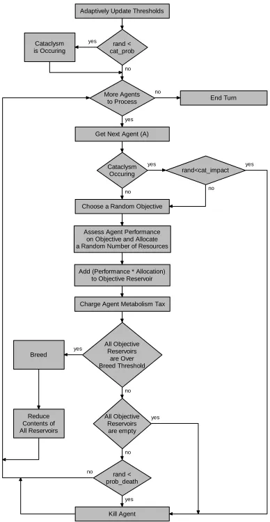
4.6 The Algorithm

Figure 1 represents a typical turn in the TB_MOO system. In the case of the first turn, a small number (less than the goal level) of agents, with randomly generated solutions, are added to the environment and the threshold is initialised with a small arbitrary number.

The system will continue to iterate through turns until the user chooses to stop the system or until some specified goal is achieved.

5 Results

Performance analysis in multiobjective optimisation has been the focus of much debate within the artificial intelligence community (Zitzler et al., 2002b; Jaszkiewicz, 2000; Van Veldhuizen and Lamont, 2000b; and Grunert da Fonesca et al., 2001). Since such debate is yet to yield a consensus approach, this paper takes a combinatory path: incorporating complexity analysis, graphical comparisons to illustrate obvious qualitative differences and further metrics to differentiate between systems with a less apparent visual hierarchy. In particular, the average distance to the Pareto optimal front and the distribution and extent of generated points in the objective space will be used to delineate key aspects of performance, while a coverage metric will analyse system dominance. For detailed descriptions of these metrics, the reader is directed to Zitzler et al., 1999.

5.1 Test Functions

The choice of test functions in any system evaluation is of pivotal importance, since it must represent the broad classes of problem that the technique will encounter in real-world use. Zitzler et al. (1999) propose six test functions (T1,…,T6) that “reflect the essential aspects of multiobjective optimisation” (Zitzler et al. 1999, p.177) and are therefore appropriate for testing the capabilities of any given multiobjective optimiser.

Consequently, TB_MOO is tested on all real-valued problems presented by Zitzler et al. (1999) – namely, T1,…,T4 and T6. Performance on binary problems, such as T5 and 0/1 knapsacks, will be explored in future work.

5.2 Comparative Systems

The performance and complexity of TB_MOO will be compared against two systems – the Non-dominated Sorting Genetic Algorithm (NSGA) (Srinivas and Deb, 1994) and its sequel, NSGAII (Deb et al., 2000). The choices here are non-arbitrary: NSGA represents a popular and well-studied approach (Zitzler et al., 1999) that has demonstrated high performance levels; while NSGAII is a contemporary

technique with the explicit aim of decreasing computational overhead. Thus, an analysis of these approaches, in conjunction with TB_MOO, will reflect the impact of computational complexity on front quality.

5.3 System Parameters

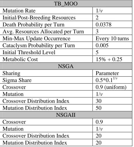
The parameters used for all tests are specified in Table 1. It is important to note that no effort has been made to produce the best parameter settings for any of the systems. For NSGA and NSGAII, the parameters are taken from system-specified defaults or otherwise from Deb et al. (2000).

5.4 Complexity

While the quality of Pareto approximations has been at the centre of most multiobjective research “optimiser performance can ultimately be understood in terms of the trade-off between the quality of solutions produced and the computational effort required to produce those solutions” (Grunert da Fonesca et al., 2001). As such, a preliminary analysis requires an investigation into the complexity of the system as a whole.

For the purpose of this analysis, the concept of complexity will be based on the number of times a solution must be referenced per generation. That is to say that the additional complexities introduced by such processes as

Adaptively Update Thresholds

More Agents to Process

Get Next Agent (A)

yes

Cataclysm Occuring

Kill Agent

rand<cat_impact

yes yes

Choose a Random Objective

Assess Agent Performance on Objective and Allocate a Random Number of Resources

Add (Performance * Allocation) to Objective Reservoir

All Objective Reservoirs

are Over Breed Threshold Breed

Reduce Contents of All Reservoirs

yes

All Objective Reservoirs are empty

no

rand < prob_death

no yes

yes

End Turn

no

no

rand < cat_prob Cataclysm

is Occuring

yes

no

no no

Charge Agent Metabolism Tax

TB_MOO

Mutation Rate 1/v

Initial/Post-Breeding Resources 2 Death Probability per Turn 0.0378 Avg. Resources Allocated per Turn 3

Min-Max Update Occurrence Every 10 turns Cataclysm Probability per Turn 0.005

Initial Threshold Level 5

Metabolic Cost 15% + 0.25

NSGA

Sharing Parameter

Sigma Share 0.5*0.11/v

Crossover 0.9 (uniform)

Mutation 1/v

Crossover Distribution Index 30 Mutation Distribution Index 50

NSGAII

Crossover 0.9

Mutation 1/v

Crossover Distribution Index 20 Mutation Distribution Index 20

Table 1 - System Parameters

v = number of variables

Table 2 – Solution References per Agent per Generation

Note that population sizes represent desired levels for threshold adaptation – experiments have found that a desired population size of 250 leads to a practical average of 319 20; 400 507 21; 550 712 50.

Population Size

System 50 100 250 400 550

NSGA 58 3 100 9 229 14 - -

NSGAII - 62 18 170 26 360 72 -

TB_MOO - - 34 1 34 1 34 1

crowding assignment, sharing and threshold adaptation will be ignored. This is reasonable as adapting thresholds in TB_MOO is a constant-time operation that is not agent-centric, while the overall complexity of NSGA and NSGAII is governed by the sorting procedure (Deb et al., 2000).

Theoretically, the worst case per-generation complexities of NSGA and NSGAII have been defined by Deb et al. (2000) as O(MN3) and O(MN2) respectively (where M is the number of objectives and N is the population size). However, the value of such a measure is debatable – it is unlikely that such computational overhead would occur in a single turn (where N unique fronts must be formed), let alone across an entire run. Consequently, it is useful to perform an empirical analysis of complexity on genuine test functions. In particular, Table 2 displays the average number of comparisons per generation for each solution (or agent), as derived from two complete runs on each test function.

While both NSGA and NSGAII are significantly lower than their corresponding worst cases, neither obtains the computational efficiency of TB_MOO. Indeed, whereas the per-agent complexities of NSGA and NSGAII are intrinsically tied to the population level, TB_MOO is divorced from this correspondence and provides a constant complexity for each agent regardless of the overall population size. The reason for this computational advantage is straightforward: TB_MOO requires no direct

agent-agent interaction.

More specifically, the per-agent complexity of TB_MOO can be defined as O(B+U) (where B is the average number of turns required for an agent to breed; and U is the number of times a solution must be referenced for min-max updates per breeding cycle). U is a system specified constant that has a practical maximum of 2B (where both the minimum and maximum values are updated every turn), which results in a worst case complexity of O(3B) O(B). Given that adaptive thresholding results in the average breeding cycle length remaining approximately constant (as evidenced by the consistent empirical values found in Table 2), the average per-agent complexity of TB_MOO is O(1). Consequently, the average per-generation complexity of the TB_MOO system is defined as O(N (1)) O(N ) (where N is the average population size).

By explicitly reducing the complexity of optimisation, TB_MOO increases the pre-existing practical limits on population size, which in-turn facilitates a more thorough exploration of the search space. The effect of such a reduction in computational complexity on front quality will be investigated in the following section.

5.5 Front Quality

0 0.5 1 1.5 2 2.5 3 3.5 4

0 0.1 0.2 0.3 0.4 0.5 0.6 0.7 0.8 0.9 1

f1

f2

TB_MOO (250) TB_MOO (400) NSGAII (250) NSGAII (400) NSGA (50) NSGA (100)

NSGA (250)

0 0.5 1 1.5 2 2.5 3 3.5 4

0 0.1 0.2 0.3 0.4 0.5 0.6 0.7 0.8 0.9 1

f1

f2

TB_MOO (250) TB_MOO (400) NSGAII (250) NSGAII (400) NSGA (50) NSGA (100) NSGA (250)

-2 -1 0 1 2 3 4

0 0.1 0.2 0.3 0.4 0.5 0.6 0.7 0.8 0.9 1

f1

f2

TB_MOO (250) TB_MOO (400) NSGAII (250)

NSGAII (400) NSGA (50) NSGA (100) NSGA (250)

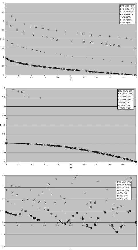
Figures 2, 3 and 4 – Front Quality of Systems for Varying Population Goal Levels with Five Million Comparisons (T1,

T2 and T3 Respectively). Reference Line = Optimal Front.

0 0.5 1 1.5 2 2.5 3 3.5 4

0 0.1 0.2 0.3 0.4 0.5 0.6 0.7 0.8 0.9 1

f1

f2

TB_MOO (250) TB_MOO (400) NSGAII (250) NSGAII (400) NSGA (50) NSGA (100) NSGA (250)

0 0.5 1 1.5 2 2.5 3 3.5 4

0.3 0.4 0.5 0.6 0.7 0.8 0.9 1

f1

f2

TB_MOO (250) TB_MOO (400) NSGAII (250) NSGAII (400) NSGA (50) NSGA (100) NSGA (250)

Figures 5 and 6 – Front Quality of Systems for Varying Population Goal Levels with Five Million Comparisons (T4

and T6 Respectively)

TB_MOO (250) TB_MOO (400)

NSGAII (250) 84 / 84 / 41 / 85 / 1 84 / 85 / 42 / 84 / 1

NSGAII (400) 54 / 1 / 37 / 4 / 0 60 / 2 / 37 / 4 / 0

NSGAII (250) NSGAII (400)

TB_MOO (250) 46 / 72 / 37 / 63 / 95 59 / 89 / 48 / 65 / 93 TB_MOO (400) 51 / 76 / 35 / 67 / 93 64 / 87 / 45 / 84 / 90

Table 3 - The Relative Coverage Percentages for Systems with Five Million Comparisons on each Test

Function (T1 / T2 / T3 / T4 / T6)

Figures 2 - 6, display the on-line results for a variety of population levels on each of the test functions. Each graph represents the amalgamation of five runs – all of which are limited to five million solution references. For the sake of clarity, only dominant solutions are illustrated, where two solutions are considered comparable so long as their difference in at least one objective is less than 0.025.

The results show that TB_MOO is consistently better than NSGA, which fails to locate the Pareto optimal front in any of the test functions. Such low quality is the direct result of the inherent complexity of NSGA, which severely inhibits the number of generations that can be produced in a given test run. In general, the problems afflicting NSGA are two fold: large populations require too much complexity to generate acceptable solutions within five million comparisons, while small populations lack the diversity required to develop the Pareto optimal front.

More importantly, in every test TB_MOO is shown to

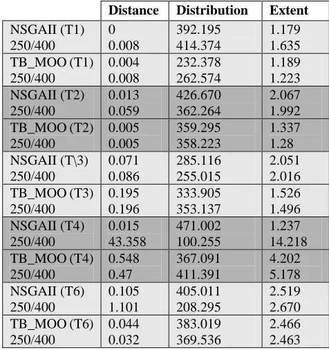
produce a good approximation of the true Pareto optimal front. That is to say that none of the tested problem features prohibit TB_MOO from achieving accurate and well-distributed fronts2. However, it is difficult to determine the marginal differences between TB_MOO and the similarly performing NSGAII graphically. Consequently, Tables 3 and 4 display the results of applying Zitzler et al.’s (1999) four quality metrics to dominant solutions from the amalgamated test runs with a finer comparison difference of only 0.001 and a neighbourhood size of 0.05.

The results illustrate that TB_MOO achieves accuracy levels that are comparable, and often better (particularly in T6), than those produced by NSGAII, but is typically less effective in terms of distribution and extent. It is likely that such deficits are influenced by lower front membership in

Distance Distribution Extent NSGAII (T1) 250/400 0.128 0.833 255.790 114.316 1.955 1.791 TB_MOO (T1) 250/400 0.009 0.499 72.634 161.394 1.189 1.791 NSGAII (T2) 250/400 0.983 1.946 63.469 37.622 2.056 1.708 TB_MOO (T2) 250/400 0.012 0.086 82.787 39.4 1.188 1.266 NSGAII (T3) 250/400 0.262 0.746 194.5 128.946 2.181 2.137 TB_MOO (T3) 250/400 0.212 0.139 8 118.281 1.331 1.514 NSGAII (T4) 250/400 139.921 161.036 46 42 14.647 12.58 TB_MOO (T4) 250/400 1.194 2.582 178.19 38.947 4.617 2.827 NSGAII (T6) 250/400 3.507 5.117 89.663 40.75 2.386 1.854 TB_MOO (T6) 250/400 0.217 0.407 302.911 111.529 2.646 2.465

Table 6 - Front Quality of Systems for Varying Population Goal Levels with One Million Comparisons

TB_MOO (250) TB_MOO (400)

NSGAII (250) 7 / 0 / 25 / 0 / 1 49 / 5 / 51 / 0 / 3

NSGAII (400) 0 / 0 / 0 / 0 / 0 17 / 0 / 1 / 0 / 0

NSGAII (250) NSGAII (400)

TB_MOO (250) 19 / 28 / 1 / 22 / 78 11 / 5 / 2 / 21 / 76 TB_MOO (400) 10 / 8 / 11 / 7 / 38 30 / 8 / 38 / 2 / 22

Table 5 - Front Quality of Systems for Varying Population Goal Levels with One Million Comparisons

Distance Distribution Extent

NSGAII (T1) 250/400 0 0.008 392.195 414.374 1.179 1.635 TB_MOO (T1) 250/400 0.004 0.008 232.378 262.574 1.189 1.223 NSGAII (T2) 250/400 0.013 0.059 426.670 362.264 2.067 1.992 TB_MOO (T2) 250/400 0.005 0.005 359.295 358.223 1.337 1.28 NSGAII (T\3) 250/400 0.071 0.086 285.116 255.015 2.051 2.016 TB_MOO (T3) 250/400 0.195 0.196 333.905 353.137 1.526 1.496 NSGAII (T4) 250/400 0.015 43.358 471.002 100.255 1.237 14.218 TB_MOO (T4) 250/400 0.548 0.47 367.091 411.391 4.202 5.178 NSGAII (T6) 250/400 0.105 1.101 405.011 208.295 2.519 2.670 TB_MOO (T6) 250/400 0.044 0.032 383.019 369.536 2.466 2.463

Table 4 - Front Quality of Systems for Varying

Population Goal Levels with Five MillionComparisons

0 0.5 1 1.5 2 2.5 3 3.5 4

0 0.1 0.2 0.3 0.4 0.5 0.6 0.7 0.8 0.9 1

f1 f2 TB_MOO (250) TB_MOO (400) NSGAII (250) NSGAII (400)

Figure 7 – An Example of Front Quality with One Million Comparisons (T4)

TB_MOO and is the direct result of the explicit inclusion of diversity preservation and elitism mechanisms in NSGAII. The incorporation of such concepts will be the focus of future work.

To investigate the speed at which Pareto optimal fronts are located, NSGAII and TB_MOO were tested again with a maximum of one million solution references (Figure 7; Tables 5 – 6). TB_MOO achieves more accurate approximations on all tests for equivalent goal population sizes and is significantly better on T2, T4 and T6 in terms of distribution, coverage and accuracy. That is to say that the reduction of computational complexity in TB_MOO provides for a genuine performance advantage over NSGAII – allowing for more rapid convergence to the Pareto optimal front.

6 Future Work

While the results presented are promising, there still exists considerable scope for the extension of TB_MOO. In particular, future work will examine the notions of elitism and diversity through the introduction of a simplified spatial model with competitive resource consumption. By including such mechanisms, front distribution and extent

should be increased, while also improving off-line performance (which has not been investigated here). Additional work may also include performance enhancement through parallelism, the inclusion of preferences in threshold specifications and adaptive mutation procedures.

Beyond system improvements, further testing and analysis is required – particularly on constraint-based and discrete problems. It will also be necessary to examine the performance of TB_MOO on problems containing more than two objectives, since these are a better representation of real-world performance.

7 Conclusions

TB_MOO is not only highly efficient – both with respect to generational complexity and front arrival – but also forms good Pareto approximations for a range of difficult problems. When tested against two prominent pre-existing systems (NSGA and NSGAII), TB_MOO consistently outperforms NSGA and produces fronts that are comparable to NSGAII (though with typically lower performance on distribution and extent). Thus, preliminary results suggest that further investigation into TB_MOO is worthwhile – particularly with a focus towards improving front diversity.

Acknowledgments

The authors would like to acknowledge the following people and institutions, without whom this paper would not have been possible: Michael Berry, Trixie Berry, Dave Benda, Sophie Darling, Claire Eden, Mark Hepburn, Ian Lewis, Pauline Mak, the School of Computing and the referees.

References

Coello, C. A. C. 1999, 'A Comprehensive Survey of Evolutionary-Based Multiobjective Optimization Techniques', Knowledge and Information Systems, 1, 3.

Coello, C. A. C. (1996) 'An Empirical Study of Evolutionary Techniques for Multiobjective Optimization in Engineering Design' Department of Computer Science, Tulane University, New Orleans.

Coello, C. A. C. 2001, 'A Short Tutorial on Evolutionary Multiobjective Optimization', First International Conference on Evolutionary Multi-Criterion Optimization, 1, 21 - 40.

Coello, C. A. C., Hernandez, F. S. and Farrera, F. A. 1997, 'Optimal design of reinforced concrete beams using genetic algorithms', Expert Systems with Applications: An International Journal, 12, 1.

Deb, K., Agrawal, S., Pratab, A. and Meyarivan, T. 2000, 'A Fast and Elitist Multi-Objective Genetic Algorithm: NSGA-II', Proceedings of the Parallel Problem Solving from Nature Conference VI, 849-858.

Fonesca, C. M. and Fleming, P. J. 1995, 'An Overview of Evolutionary Algorithms in Multiobjective Optimisation', Evolutionary Computation, 3, 1, 1-16.

Fonesca, C.M. and Flemming, P.J. 1998. 'Multiobjective Optimisation and Multiple Constraint Handling with Evolutionary Algorithms - Part I: A Unified Formulation', IEEE Transactions on Systems, Man and Cybernetics - Part A: Systems and Humans, pp. 26-37

Goldberg, D. E. (1989) Genetic Algorithms in Search, Optimization and Machine Learning, Addison-Wesley, Massachusetts.

Goldberg, D. E. and Richardson, J. 1987, 'Genetic Algorithms with Sharing for Multimodal Function Optimization', Genetic Algorithms and Their Applications: Proceedings of the Second International Conference on Genetic Algorithms.

Grunert da Fonesca, V., Fonesca, C. M. and Hall, A. O.

(2001) 'Inferential Performance Assessment of Stochastic Optimisers and the Attainment Function' Evolutionary Multi-Criterion Optimisation, First International Conference, Vol. 1993 (Eds, Zitzler, E., Deb, K., Thiele, L., Coello, C. A. C. and Corne, D.), pp. 213-225.

Jaszkiewicz, A. (2000) 'On the Computational Effectiveness of Multiple Objective Metaheuristics' Fourth International Conference on Multi-Objective and Goal Programming (MOPGP) (Eds, Traskalik, T. and Michnik, J.) Springer-Verlag, Berlin, Heidelberg, pp. 86-100.

Knowles, J. and Corne, D. (1999) 'The Pareto Archived Evolution Strategy: A New Baseline Algorithm for Pareto Multiobjective Optimisation' Proceedings of the Congress on Evolutionary Computation, Vol. 1 IEEE Press, Washington, D.C., pp. 98-105.

Laumanns, M., Rudolph, G. and Schwefel, H.-P. (1998) 'A Spatial Predator-Prey Approach to Multi-Objective Optimization: a Preliminary Study' Fifth Conference on Parallel Problem Solving from Nature (Eds, Eiben, A. E., Back, T., Schoenauer, M. and Schwefel, H.-P.) Springer, Amsterdam, pp. 241-249.

Socha, K. and Kisiel-Dorohinicki, M. (2002) 'Agent-Based Evolutionary Multiobjective Optimisation' Proceedings of CEC 2002 - Congress on Evolutionary Computation, Vol. 1.

Srinivas, N. and Deb, K. 1994, 'Multiobjective Optimization using Non-dominated Sorting in Genetic Algorithms', Evolutionary Computation, 2, 3, 221 - 248.

Van Veldhuizen, D. A. and Lamont, G. B. (1998) 'Multiobjective Evolutionary Algorithm Research: A History and Analysis' Department of Electrical and Computer Engineering Air Force Institute of Technology, pp. 88.

Van Veldhuizen, D. A. and Lamont, G. B. 2000a, 'Multiobjective Evolutionary Algorithms: Analyzing the State-of-the-Art', Evolutionary Computation, 8, 2, 125 - 147.

Van Veldhuizen, D. A. and Lamont, G. B. (2000b) 'On Measuring Multiobjective Evolutionary Algorithm Performance' Congress on Evolutionary Computation 2000.

Zitzler, E., Laumanns, M. and Thiele, L. 2002a, 'SPEA2: Improving the Strength Pareto Evolutionary Algorithm For Multiobjective Optimization', Evolutionary Methods for Design, Optimization and Control.

Zitzler, E. and Thiele, L. 1998, 'Multiobjective Evolutionary Algorithms: A Comparative Case Study and the Strength Pareto Approach', Lecture Notes in Comp. Science, 1498.

Zitzler, E., Thiele, L. and Deb, K. (1999) 'Comparison of Multiobjective Evolutionary Algorithms: Empirical Results' 1999 Genetic and Evolutionary Computation Conference, Vol. 8 (Ed, Wu, A. S.) Orlando, Florida, pp. 173-195.