Differential techniques for the accurate estimation of image flow

(1)

Differential Techniques for the

Accurate Estimation of Image Flow

by

Andrew S. L. Bainbridge-Smith, B.E.(Hons.)

Department of Electrical and Electronic Engineering

submitted in fulfilment of the requirements

for the degree of

Doctor of Philosophy

(2)

THE

uNniERSITY

Tat\IIPMIA

wye

,NRY

El e Ele

c

ffor„c

(3)

Statement of Originality

This thesis contains no material which has been accepted for the award of any other degree or diploma in any tertiary institution. To the best of my knowledge and belief, the thesis contains no material previously published or written by another person, except when due reference is made in the text.

Authority of Access

This thesis may be made available for loan and limited copying in accordance with the Australian Copyright Act 1968.

(4)

Abstract

One of the prime objectives of many robotic systems is the ability to judge depth for self navigation. This depth or range information in a three-dimensional scene has traditionally been obtained from point correspondences in static two-dimensional images, a process often known as photogrammetry. This approach has the major difficulty that point pairs corre-sponding to a common three-dimensional scene point are not easy to identify automatically in images. In more recent years a wide range of alternative approaches for estimating depth have emerged. One such group of techniques makes use of multiple images from a single moving sensor. Known as shape from motion algorithms, they often employ a three step process to estimating depth. The first step involves estimating the optical or image flow. The second step then estimates the global motion parameters of the image sensor from the image flow. The final step involves estimating the relative depth from the image flow and motion parameters. Thus in order to make reliable depth estimates, accurate image flow measures are required. This thesis, therefore, concentrates on the detailed analysis of techniques employed for accurately determining image flow.

Preliminary chapters introduce basic computer vision concepts and image flow algorithms. As some of the terminology used in this field is ambiguous, particular care has been placed on presenting a well defined set of terms, notably defining: "camera motion", the "motion field", "optical flow" and "image flow". Also defined is the "aperture problem" which describes a fundamental inability to perceive or measure motion in directions were no change in the image intensity function is present. It is demonstrated that all techniques rely on the presence of non-zero second order differential terms of the image sensor intensity function to overcome the aperture problem.

(5)

vi

ABSRACT

possible. Based on this criteria it is concluded that the technique based on a weighted least squares solution of first order differential terms of the image intensity is the best generalized second order method for achieving this objective.

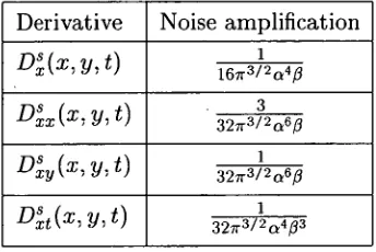
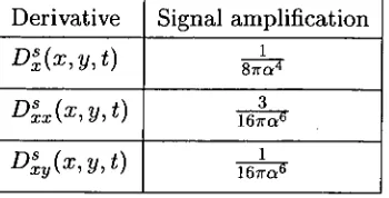
The practical issues of regularization of the gradient calculations and the influence of noise corruption are investigated. Conclusions drawn show the importance of smoothing and the effects of excessive smoothing, including a loss of spatial precision and an increase in numer-ical error due to the computation of small gradient terms. Importantly it is demonstrated that spatial and temporal gradients are not independent and consequentially their respec-tive errors are correlated. It is thus shown that many image flow estimation techniques exhibit a systematic bias.

An investigation into methods of assessing the quality of image flow estimates is also made. Indicators of the quality of an estimate are required in order to evaluate the accuracy of subsequent estimates made from them; particularly depth estimates, segmentation of the image flow field, and determining the optimal aperture size for making image flow esti-mates. Findings illustrate that the correlation between many commonly used, or proposed, indicators of image flow error are poor.

Some investigative work into two innovative approaches for estimating image flow, based on the use of colour and actual camera motion parameters, is presented. It is shown that both colour and camera motion parameters provide an additional constraint to the estimation procedure, which can be used to improve the resolution of the image flow field by allowing smaller apertures to be considered. Preliminary results from these studies suggest that both sources of additional information improve the robustness of the algorithms.

(6)

Acknowledgements

This thesis culminates four and a half years of thought, turmoil, torture and worry on more than my own behalf. To the many people who have suffered, and hopefully gained from this effort, I offer my heart-felt thanks. In particular, my extreme appreciation and thanks must go to my supervisor Dr Richard Lane who not only has provided much in the way of teaching, discussions and criticism but also tolerance for my ever lateness in getting things done.

A doctorate is a challenging journey, one I would not have undertaken if it were not for the initial encouragement of others. My most sincere thanks to my parents who have instilled in me an appreciation of the importance of learning, striving for the limits of ones talents, and a pinch of old-fashioned curiosity. Their encouragement and those of my siblings, Jeremy, David and Sarah have been undiminishing. My thanks also to Dr Bernard Guillemin at the University of Auckland, who in my last year at Auckland advised me honestly and wisely about the difficulties and rewards of undertaking such a programme.

I arrived in Hobart in March 1992 as an almost complete stranger. Though not a doctor some three years earlier, Dr David McLaren had kindly taken the time to talk to me about his experiences of doing an engineering degree. In Hobart as a doctoral student, he again took the time to talk to me about his enjoyment of doing a PhD, and also to help find accommodation, instill the proper study ethos and generally making me feel welcomed. To the other PhD students, particularly Dr Marc Stoksik, soon to be doctors Andrew Innes and Jason Pieloor go my appreciation for their help both academic and otherwise and for their unfaulting friendships. I shall always miss our morning coffee breaks, lunch-time indoor soccer, afternoon tennis matches and late evenings either working or playing computer games!

(7)

Viii ACKNOWLEDGEMENTS

particular to my associate supervisor Professor D.T. Nguyen, Tasmanians: Dr Jon Osborne and Glen Mayhew and Cantabrians: Associate Professor Peter Gough (for allowing me to use Canterbury's resources), Dr Phil Bones and Dr Adam Schwartz, and PhD students David Hawkins, Maria Luiza Lisboa, James Preddey and Volker Kuhlmann. This study would not have been possible with out the financial assistance of an Australian Postgradu-ate Award through the University of Tasmania, and the support of my parents and partner.

(8)

Preface

I arrived at the University of Tasmania in Hobart at the beginning of March 1992 to undertake a programme of study towards a PhD, having completed a bachelors degree in electrical and electronic engineering from the University of Auckland. My initial studies at the university concentrated on parameter estimation and least squares analysis which led into my first project concerning the training of neural networks. The initial hope of this work was to come up with a fast method of training a neural network for classifying Fourier descriptors of edge detected images. A conference paper on the training method was written and presented in Melbourne in early 1993. However, the result of this work was to spawn my interest in image processing rather than neural networks.

(11)

xii

PREFACE

In coming away from this work I hope that the reader will appreciate that although there is much published work in the field, many of the algorithms have a common base. In essence there are only two types of algorithm which can either be implemented in space-time or Fourier domains. This work concentrates mostly on differential techniques in the space-time domain and clearly shows that a local least squares method is best. Other results show the necessary requirements of regularizing derivative measures, the inadequacy of many published methods for indicating erroneous image flow measures, and significantly that the estimated image flow is likely to exhibit a systemic bias in its measure.

Chapters 5 and 6, although not consisting of a great proportion of this thesis, required a considerable effort. I easily spent some six months learning to control an industrial robot, becoming familiar with quaternion algebra, calibrating cameras and other implementation requirements. In some respects I found this work very rewarding; it was practical. However, in the end, mechanical jitter, instability and poor accuracy of the robot system meant that much of the data obtained from this source was unusable. Vision systems are, as of yet, not robust enough to handle pixel jitter in the order of 6 pixels/frame! There is much yet to be done in this exciting field, and I hope the reader is left with the same level of excitement that I had in developing and writing this work.

Thesis Organization

(12)

PREFACE

xiii

Supporting Publications

This research has resulted in two journal papers and a number of conference publications.

These are listed below:

• A. Bainbridge-Smith, M.A. Stoksik and R.G. Lane, "Optimization of Multi-layer Neural

Networks using Gauss-Newton Minimization", in the Proceedings of the Fourth

Aus-tralian Conference on Neural Networks (ACNN '93), Melbourne, Australia, pp.114-117,

Feb. 1993

• A. Bainbridge-Smith and R.G. Lane, "Incorporating the Aperture Problem into Optical

Flow Measurement", in the Proceedings of the First New Zealand Conference on Image

and Vision Computing (IVCNZ '93), Auckland, New Zealand, pp.431-438, Aug. 1993

• A. Bainbridge-Smith and R.G. Lane, "Statistically Based Computation of Optical Flow",

in the Proceedings of DICTA-93, Australian Pattern Recognition Society, Sydney,

Aus-tralia, pp.228-235, Dec. 1993

• R.G. Lane, N.F. Law and A. Bainbridge-Smith, "Ensemble Deconvolution using a

Wave-front Sensor", in the Proceedings of DICTA-93, Australian Pattern Recognition Society,

Sydney, Australia, pp.236-243, Dec. 1993

• A. Bainbridge-Smith and R.G. Lane, "Measuring Image Flow from Colour Imagery", in

the Proceedings of Electronic Colour Imaging and Applications Workshop (DICTA-94),

Australian Pattern Recognition Society, Canberra, Australia, pp.9--14, Dec. 1994

• A. Bainbridge-Smith and R.G. Lane, "Generalised Differential Optical Flow", in the

Proceedings of IVCNZ-95 Workshop, Lincoln, New Zealand, pp.113-118, Aug. 1995

• A. Bainbridge-Smith and R.G. Lane, "Consistent Optical Flow", in the Proceedings of

DICTA-95, Australian Pattern Recognition Society, Brisbane, Australia, pp.673-6'78,

Dec. 1995

• A. Bainbridge-Smith and R.G. Lane, "Measuring Confidence in Optical Flow

Estima-tion",

IEE Electronic Letters,

32(10), pp.882-884, May 1996.

(13)

Glossary

Symbols and Abbreviations

0

a

'Y

A

IF 1:

IF2:

IF3:

IF4:

IF5:

IF6:

IF7:

IF8:

IF9:

IF 10:

Convolution operator

Quaternion multiplication operator

Spatiotemporal smoothing coefficient

Window size and weighting coefficient for local first order gradient technique (IF5)

Weighting coefficient for Horn and Schunck's (IF4) smoothness constraint

Weighting coefficient for the augmented second order gradient technique (IF6)

Singh and Allen's original correlation method of computing image flow.

A variant of Singh and Allen's correlation method.

Horn and Schunck's differential method of computing image flow.

Local first order differential method of computing image flow.

Local augmented second order method of computing image flow.

Local second order method of computing image flow.

A variant of method IF4 that incorporates colour information.

A variant of method IF5 that incorporates colour information.

A variant of method IF5 that incorporates known camera motion parameters.

Terms

• Motion Parameters:

(14)

GLOSSARY XV

• Camera Motion or Egomotion:

Movement of the camera relative to the scene according to its motion parameters. Egomotion means self motion.

• Motion Field:

Scene points move with velocities in 3D space relative to the camera as a result of camera motion, this collection of velocities is called the motion field. •

• Optical Flow:

The perspective transformation of the 3D motion field velocities into 2D space defines a field of 2D velocities. Optical flow is thus geometrically related to the motion field. Depending on context the optical flow may refer to the entire field or a point within the field.

• Image Flow:

•An estimate of the optical flow made from a sequence of images. This is a calculated quantity made from measured data and hence only approximates the optical flow. Depending on context this may refer to the entire field or a point within the field.

• Aperture Problem:

The inability to observe or measure all components of the optical flow, especially in directions parallel to the spatial gradients of the image intensity.

• Vernier Flow:

A field of velocities, or depending on context a point within a field, where the velocity at a point is only known in one direction (vernier direction). This direction is usually parallel to the spatial gradient of the image intensity, and arises from measurements made from data suffering from the aperture problem.

• Needle diagram, Flow field diagram:

A diagram illustrating an optical, image or vernier flow field. Each vector shows both direction and magnitude of the movement of a picture element.

• BRDF:

(15)

xvi

GLOSSARY

• Chromaticity:

A term that collectively describes the two colour components hue and satura-tion. These describe the colour but not the intensity of light.

• Achromatic:

(16)

Chapter

1 Introduction

The rapid development in the mid 1970's of robotics has in part been due to the advent of cheaper computing power made possible by integrated circuitry. This has seen a progression from simple automated manufacturing techniques, such as those initially used in mass car production, to sophisticated production lines which require substantially less human input within the actual production cycle. Robots are well suited to performing the repetitive tasks which are common-place in most production cycles, as their "concentration" and "attention" never wane from the programmed job. From an engineering point of view, robotics offer multi-functional machines that can rapidly change tasks, often within minutes or even seconds. This results in a flexible, programmable production line. These production lines can be "re-programmed" within weeks instead of the months required in many "hard-wired" or fixed-automated environments, or alternatively, those simple and totally non-automated environments.

Popular science fiction, and much of the public perspective, have viewed robots as intelligent machines with human features; bipeds with two arms with 5 fingered hands, and a head with eyes, ears, nose and a mouth. Isaac Asimov, is one of the principal authors who has helped foster this public perception through his fictional work on robots and computing [33]. The word robot is derived from the Czech robota, meaning compulsory labour or "to work" in other Slavic languages [41]. Its modern sense stems from the Czech playwright Karel 'Capek and his work "R.U.R." (Rossum's Universal Robots).

(17)

2 CHAPTER 1. INTRODUCTION

The mechanics of a human-like machine are extremely complex, research is still attempting to develop a hand of similar dexterity, strength and sense of touch as our own human hands. Additional to the mechanical issues are the sensory requirements of sight, hearing, smell, taste and touch, as well as control and other knowledge requirements. Asimov's robots were adept at performing "simple" tasks such as domestic and cleaning duties, hazardous tasks and the mundane, even within the same environment as their human supervisors.

These tasks are, however, anything but simple. The vision process alone poses one of the most difficult because of the large volume of information that must be processed. One second of a standard TV signal consists of approximately 6MB of data [35, 36, 38, 42]. It is therefore not unreasonable to question the need to research and develop machinery that mimics human functions. In order to answer this question we must clearly understand our expectations from such research. From a medical perspective much of the mechanical work is valuable in terms of prosthetics. However, from an engineering or manufacturing stand-point such value is unlikely. Nonetheless, much of the research into sensory functions could prove useful, for example the use of vision in object recognition and navigation. It is, in fact, the lack of these additional sensory abilities that has seen a limiting in the interest in robotics by industry. Hence, although we are likely to see the development of many of the functional units required to develop a human-looking robot, it is less likely that these units will be put together to build such a machine.

While current machines are orders of magnitude more flexible task wise than their prede-cessor, they are nevertheless still limited to fixed programmed movements and are largely oblivious to their surrounding environment. For robotics to move forward we must add sensory abilities to our machines. Indeed they are required in order to develop such systems as industrial carpet cleaners, automated warehouse storage, high-tech surveillance and so on, as industry and consumers demand.

1.1 Robotic Vision

(18)

1.1. ROBOTIC VISION 3

doing so is unsafe, or touch will lead to an undesirable change in the world.

Take as an example, a situation of being placed in a vast expanse of flat grassland in which a wandering pride of hungry lions is also located. Early identification of the pride is essential in order to take evasive action. Touch is not possible from an issue of safety, and because vision is non-invasive to the environment, retreat without giving away your location is possible. There is much to be said for letting sleeping lions lie!

Human interest in vision, has extended from the hunter/gather/survival requirements, which we rather take for granted, into fields of scientific and engineering endeavour. Initially this was through astronomy which aided farming and navigation. Vision was looked upon as a useful tool in this regard, although it was not until the likes of Newton etc., that an interest in light and the vision process started to develop [1]. Interestingly, a comprehensive connection between the vision process and geometry was only formed in the mid 1800's [2, 37]. With the advent of the camera came surveying from photographs, [1, 2]. Called photogrammetry the field quickly developed and these same techniques form the cornerstone of many machine vision algorithms [1, 2,10, 14].

Machine vision looks at solving the problem of making value judgements from the recog-nition of objects within the image, and, or the measurement of features within the image. These tasks we perform "effortlessly" with our 10 12 odd neurons [37]. Despite the develop-ment of ever increasingly computationally powerful computers, these computers are never-theless no where near the ability of even emulating the common house fly in its ability to navigate a hazardous environment. This is of course a difficult problem. Fortunately some success has been achieved for much simpler tasks, such as self navigating laboratory robots where the environment is highly controlled. This has been driven by strong research evidence in neurobiology, neuroanatomy, psychophysics, and psychology that suggest cues such as shading (image intensity variation), texture (distribution of surface markings), contours and line-drawings, motion and stereo are very helpful in deducing properties of three-dimensional surfaces from their visual images [49-51, 74, 84, 94, 95, 116, 150, 173, 187, 188, 208, 216, 217].

(19)

--- epipolar line

t - , _{_}

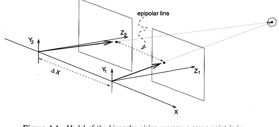
Figure 1.1: Model of the binocular vision process; a scene point is im-aged onto two separate sensors separated by a distance AX . The two image points line on the epipolar line which runs parallel to the X axis. The difference of the ordinate values of the imaged points from their respective axes is related to the distance of the object and the sensors separation.

a process which has been utilized for many years by surveyors. The technique relies on locating common points in the three-dimensional scene from images taken from multiple separate cameras or a moving camera over time. It is the same binocular vision process by which many animals, ourselves included, see. Figure 1.1 illustrates this process. Comparing the disparity or difference between the scene points position in the two views, and given the

[image:19.571.44.492.110.314.2]

(20)

1.2. VISUAL MOTION 5

1.2 Visual Motion

In more recent years a wide range of new approaches for estimating depth have emerged, including: shape from shading, shape from texture, depth from focus, and shape from motion [45,49,53,59,68,86,92,101,108,117,125,128-131,133,141,142,160-162,168-171,177, 179,196,202,203,209,218,221,222]. In the first two cases, depth information is inferred from a single image only. Shape from motion and depth from focus algorithms differ in that they make use of multiple images. Depth from focus can be considered, however, as a special case of shape from motion, as it utilizes the disparity between two images caused by changing the focal length and knowledge of the camera's intrinsic parameters to estimate depth. Provided the motion parameters of the camera are known and the intrinsic parameters of the camera are not changed, shape from motion algorithms, which use just two images, are equivalent to measuring a binocular image pair. Other motion based algorithms, which make use of more than two images, can be thought of as binocular vision techniques enhanced by the ability to track points over long sequences.

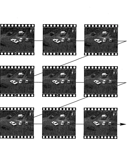
Motion analysis is most commonly performed on an image sequence obtained from a single camera, although some approaches based on the motion of stereo cameras have also been considered [83,137,159,218,219]. It is the monocular vision approach that is adopted in this work, due to its simplicity and cost effectiveness (utilizing only one camera). An example of a monocular image sequence is shown in Figure 1.2. This is the "Hamburg Taxi" image sequence which is one of a number of freely available standard image sequences. Appendix A illustrates examples of all the image sequences used in this thesis, along with information about where they may be obtained.

(21)

40 11 0 41 10 0 40 10 11 40

10 11 40 411 CD 0 40 40 0 0

11 40 40 11 0 40 0 11 0 11

0 40 10 40 C) 0 40 0 40 40

10 0 10 11 10 0 11 411 0 11

• 0 410 11 41 10 40 11 10 11

41 1/ 11 0 0) 11 0 41 41 411

40 11 0 11 C) 0 11 41 41 41

11 0 41 40 41 41 41 11 10 11

11 41 0 411 11 41 0 41 411 41

41 11 0 41 411 11 40 41 0 11

40 41 0 40 0 11 41 0 11 11 0 11 0 0 0 11 41 0 411 0 411 10 11 11 (ID 11 0 0 40 0

6

CHAPTER 1. INTRODUCTION

[image:21.568.51.493.123.607.2]

(22)

1.2. VISUAL MOTION 7

Figure 1.3: Circles highlight the movement of objects from the first frame (left) to those of a later (right).

Figure 1.4: Taking a difference image of the two frames shown in Figure 1.3 shows that the circled objects have moved.

limitation is that this method is only suitable for situations where the camera is stationary and the background constant.

(23)

n rt. A-

k R RFC

Figure 1.5: A needle diagram showing the movement of picture elements in time. This flow field was computed about the 9th frame in the Ham-burg Taxi sequence using the author's implementation of Horn and Schunck's image flow algorithm.

can be constructed by performing a point-wise match of each pixel in one image to a pixel in the other. However this is a nightmare computationally, with a potential of N 2 matches, where N is the total number of pixels per frame. Furthermore, if pixel intensity is the sole basis of comparison, then the algorithm is likely to suffer from many equally likely matches.

Two more needle diagrams are shown in Figures 1.6 and 1.7. These are computed for synthetic image sequences which were created from the simulated motion of a camera looking at a tree. Like the estimate for the Hamburg Taxi sequence they are computed using Horn and Schunck's algorithm [102] which is presented later in this thesis, along with other algorithms that provide computational superior alternatives to the point-matching approach. These diagrams also illustrate another feature of the algorithms to be presented, the ability to compute a dense flow field.

(24)

p.

, ...:::•-•

t'

4...,4..4 V

I. 1,. ..

:*

4

4-- ÷ t.".A.:74" ..*

4. 4 .-,-.). ,)• —1 - - s. *S44 :

* I.#

*Afi44- "4.44 _...;NAi .4

1 ','' *.:**. 1! * 4t-":* * -V * 1.1 1.i

--'* *,* * 4i 1 N ). iiri

■ i

i1:.''* ''.."2,

..-`*. '.)f .t#:'..'4

Ae,.*

1..14, le 44

1.2. VISUAL MOTION 9

Figure 1.6: Estimating the image flow for frame 20 from the Translating Tree sequence using Horn and Schunck's method.

(25)

be made about how to interact with the world. In a robotics environment such decisions form the basis of controlled motion, and thus it seems eminently sensible to use the information gained during movement to refine the control process. Vision therefore provides a potential feedback process to motion control. The key to success of the feedback process is the accurate measurement of image flow.

Although the approach taken and developed in this thesis is designed for robotic vision, the measurement of image flow has successfully found commercial application in such fields as image compression for High Definition Television (HDTV), and the estimation of wind speed and ocean currents for meteorological forecasts and climate studies [3,140,164,174,180,230]. Other applications include measuring plant growth, tracking cataracts and flight-systems to assist pilots [57, 98, 189]. As in the case of robotics, dense flow fields are required along with some indication of the reliability of each measure. Resolution, density, accuracy and reliability of image flow are therefore the prime factors considered when comparing the performance of various techniques.

1.3 Thesis Structure

This thesis presents various techniques for the accurate estimation of image flow. The topic is presented in a manner that develops these techniques for inclusion in an active vision system. The thesis is written in a style that groups together common topics into single chapters, with accompanied relative experimental work. However, only brief conclusions are drawn in these chapters as a single comprehensive conclusion is left to the last chapter. This allows a discussion of common results which span more than one chapter.

Firstly, a discussion of image formation and camera motion is made at the beginning of Chapter 2. A formal definition of image disparity, called optical or image flow, is then presented along with the fundamental obstacle faced by all algorithms based on measuring image disparity, namely the aperture problem. Finally, Chapter 2 presents prerequisite knowledge on the numerical techniques required by practical systems as well as the method by which errors in the disparity estimates can be measured.

(26)

1.3. THESIS STRUCTURE 11

tationally efficient. A brief comparison of algorithms from both of the two classes is made on a number of image sequences. The chapter concludes with a detailed investigation of Horn and Schunck's differential method with comparisons to results obtained by Barron et al.[54] for their implementation of this algorithm. Such analysis and comparisons are essential in order that any enhancements made are meaningful and addresses the criticism;

"Computer Vision suffers from an overload of written information but a dearth of good evaluations and comparisons."

Price[175]

It is fortunate that in the field of image flow analysis some recent efforts to address this criticism exist, [54-56,167,226], especially the work of Barron and others at the University of Western Ontario. Unfortunately, some of these results were in error, in particular their implementation of Horn and Schunck's algorithm. The results presented in this thesis therefore substantially differ from those of Barron et al., [52,132].

Chapter 4 extends the detail of this comparative work, concentrating on the class of dif-ferential or gradient based techniques for measuring image flow. Comparisons are made with respect to the resolution, density and accuracy of the image flow. Noise analysis and estimator reliability are also investigated since, these are crucial to estimating the reliability of depth estimates.

In Chapter 5 investigations of two innovations for improving flow estimates are made. Both relate to the inclusion of additional information. The first considers the effect of colour information. The cost of "off-the-shelf" colour cameras is comparable to many greyscale (monochrome or black-and-white) cameras, making the purchase of this style of sensor attractive to a number of researchers. The second considers the affect of assuming that the camera motion is known a priori. This is not an unrealistic assumption as the control algorithm moving the camera can, at least in part, supply this information. Inevitably though this information will be partially erroneous, due to noise and mechanical effects, such as slippage, which give rise to inaccurate measurements. The effects of these errors are briefly investigated.

(27)

nately, there is a lack of suitable real image sequences which have known camera motion. Consequently many of the results presented in this chapter are also of a qualitative nature.

(28)

Chapter 2 Background

This chapter introduces the concepts of image formation, camera motion, optical and image flow, and related practical issues. The objective is to clearly define the terminology used and in this regard we make a clear distinction in the use of the terms optical and image flow. The former is a geometric term that is exact and independent of the image formation process, while the later is an estimated quantity resulting from noisy image measurements. In clarifying the distinction between these terms, it is necessary to develop an understand-ing of the conditions which affect the accuracy of measurunderstand-ing movunderstand-ing picture elements. The most significant difficulty faced by any image flow algorithm is over-coming the aperture problem. A discussion of the sampling theorem for moving pictures, numerical techniques and other practical requirements demonstrates the effects of some of the principal simpli-fying assumptions. Finally, an important discussion on error metrics is made, as in reality an estimate of unknown accuracy is only marginally more useful than no estimate at all.

2.1 Image Formation

The process of image formation is crucial in order to develop a greater understanding of the process of how pictures change in time. Two distinctive processes are involved in the image formation process: how energy is radiated from a scene, and how this energy is measured.

(29)

14 CHAPTER 2. BACKGROUND

Measuring Process

The measurement process involves collecting the energy emitted from the scene on an ap-propriate sensor. In machine vision problems, the sensor is typically a camera based on a two-dimensional CCD array. Consequently, the image plane of the camera is modelled as a set of cells mapped out on a rectangular grid (see Figure 2.1) where each cell measures the amount of energy it receives over a period of time. The measured photon count in each cell is then digitized for further processing by a computer system.

The correspondence between a point in the scene and its image on the image plane depends on the relative position of the scene point to the camera sensor, and the intermediate optics of the camera lens. The mapping between scene and image points is defined by the perspective transform,

[ zy

1= [

zzy

(2.1)

where uppercase letters, (X,Y,Z), denote the three-dimensional coordinates of scene points

and lowercase letters, (x, y), denote the two-dimensional coordinates of image points. All

light rays incident on the image plane must pass through the focal point which is at a distance f from the plane, Figure 2.2. The number of photons exciting the cell is dependent

on the position of the scene relative to the sensor, the attitude and reflectance properties

(30)

2.1. IMAGE FORMATION 15

Figure 2.2: Scene points in the three-dimensional coordinate system (X, Y, Z) are projected onto the two-dimensional sensor or image plane (x, y) at a distance f from the origin. The two coordinate systems are related by the perspective projection.

of points in the scene, and the distribution of light sources.

Radiometry

The amount of light falling on a surface is called the irradiance, and is measured in power

per unit area (Wm -2 ). The amount of light radiated from a surface is called the radiance,

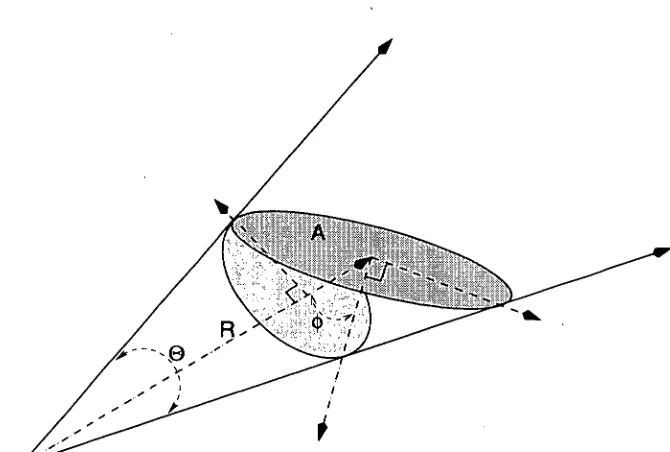
and is measured as the amount of power per unit area of unit solid angle (Wm -2rad -1 ). The radiance measure is complicated because the source can radiate light into many differing directions with varying amounts of energy. In order to define this we need to compute the light radiated in a given solid angle, where the solid angle is defined as an angle equal to the area cut out by a cone on the unit sphere. Figure 2.3 shows a small planar patch of area A at a distance R from the origin with an attitude angle of 0. The foreshortened area,

or effective area oriented towards the origin (illustrated by the lighter grey region), is equal to A cos 0 and thus subtends a solid angle,

A cos 0

0

R2 (2.2)

of the unit sphere.

In Figure 2.4 we see that the light radiating from a scene patch 80 with an attitude 0

to the centre of the lens has an effective area of 80 cos towards the lens. This light is

(31)

in the direction of 0 is given by L then the power emitted by the patch is,

6P = L60 cos (0) /2, (2.3)

where 12 is the solid angle subtended by the lens as seen by the object and represents the light catching potential of the lens for the scene patch, Figure 2.5. The lens has an area id2 with an attitude of a to the scene patch. Given that the distance between lens and object is Z/ cos a, then by substitution of these relationships into Eq.(2.2) the solid angle is defined by,

F-d2 cos a =

(Z/ cos a) 2

Since this power is concentrated in the image and assuming no losses in the lens, the irradiance measured by the cell will be,

6P 60 1= —

s = L—s cos (0) C2.

The solid angle subtended by the image plane cell, 5, to the lens is equal to the solid angle subtended by the object patch, 60, to the lens, as evident in Figure 2.4. Hence,

S

cos ce =

60 cos 0 ( f /

cos ce)

2 (Z/ cos a)

2

60 cos a (Z 2

(2.6)

S cos 0 f

By substituting Eq.(2.6) into Eq.(2.5) the irradiance of the measuring cell is given as,

2

I = L cos (a) (--f-Z ) it

= L

cos4 (a) (1) . 2 (2.7)

Since the angle of view, a, is typically narrow, Eq.(2.7) is insensitive to the fourth power cosine term. Moreover other factors, such as vignetting effects (power loss in a lens system, see [7]), are usually more significant, and in practice the fourth power cosine term can usually be ignored. We thus note that the irradiance measure is proportional to the scene radiance and the square of the reciprocal f-number (f/d) .

(2.5)

(32)

[image:32.563.119.454.95.321.2]

Figure 2.3: The base area of a cone (lighter grey area) at a distance R

from its origin is defined by its solid angle 0. The general surface A can be reoriented towards the cone by the cosine of the angle, 0, the normal makes with the centre-projection of the cone.

[image:32.563.104.507.385.670.2]

(33)

A

Figure 2.5: The light catching potential of a lens is restricted by its aperture size d.

example of a surface which concentrates the reflected light from a point source in only a very narrow angle. The mirror example clearly shows that the radiance of a surface depends on its physical properties, as well as the direction of illumination and the direction from which it is viewed. The surface physical property can be described by the Bidirectional Reflectance Distribution Function (BRDF) [101, 160]. In a coordinate system local to the scene point the BRDF can be defined in terms of the polar angle and azimuth of the incident and emitted rays,

Oi; 0e, 0e) = (5/(0i, 0i)

where 6.1(0i, 0i) is the incident irradiance and 8L(Oe, .0e) is the emitted radiance.

The BRDF can be determined experimentally, but this is difficult and tedious because it has four degrees of freedom. Furthermore, it is impractical in realistic situations where the scene, and consequently the BRDF, is unavailable a priori. Notwithstanding this difficulty, the BRDF will lie between two extremes: one of all light being reflected at an angle determined by its incidence; and the other being light scattered independently of its angle of incidence.

An ideal specular surface reflects all light arriving from the direction (0,, Oa) into the

di-rection (9j , —0,). This is typified by a perfect mirror surface, shown in Figure 2.6. In this case,

L(O

e

, 95_{,) = I(ei,} (2.9)

8L(0e, 0e)

(2.8)

(34)

■

,.... , .... NORMAL ---

VIEWER

—E-

SOURCE

(35)

(a) (b)

Figure 2.7: Lambertian reflective spheres: (a) illuminated by a point source, (b) by an extended or diffuse light source.

bright from all viewing directions and reflects all incident light. In this case the BRDF is a constant. Horn [7] shows that for a Lambertian surface illuminated by a point source,

L = *I cos (2.10)

which is Lambert's cosine law of reflectance from matte surfaces. For an extended or diffuse light source,

L

=

(2.11)

Figure 2.7 shows two examples of a Lambertian sphere lit by a point source and an extended source. In the case of a point source the image surface appears curved due to the brightness variation, Figure 2.7(a). The image taken under an extended light source appears as a flat disk, Figure 2.7(b). In this case all sense of depth is lost in the image, a phenomena often referred to as "white out".

2.2 Camera Motion

[image:35.566.53.498.103.339.2]

(36)

2.2. CAMERA MOTION 21

of weather forecasting for instance, a geostationary satellite (stationary sensor) monitors moving cloud patterns and ocean currents. However, in the example of an autonomous robot navigating though an automated storeroom the sensor is moving though a static scene. Most authors argue that the distinction is relative and dependent only on one's point of reference. However, as presented in the previous section on image formation, the BRDF of a surface is functionally dependent on the orientation and position of the scene to the light sources. Therefore the two forms of motion, from a radiometry point of view, are not equivalent. We consider this issue in greater detail in Section 2.4 where a number of common assumptions are considered. For consistency in this work the situation where the scene is chosen to remain static while the camera is allowed to move is the primary mode of operation.

Camera position and orientation in the three-dimensional world are described by 6 para-meters. Position is most conveniently represented in rectangular coordinates, (X, Y, Z).

Orientation is usually represented in terms of the angles, roll (a), tilt (0) and pan (-)6) , (also called roll, pitch and yaw), but may also be described as Euler parameters or quaternions. Roll, pitch, yaw angles usually lead to a rotation matrix description, but a quaternion representation affords a number of significant advantages, in particular a more compact description (see Appendix B). Quaternions are the form used in Chapter 5 when we discuss camera motion in greater detail.

If the camera is now allowed to move with constant translation component,

T

=

w

v

(2.12)

and constant rotation component,

Q = [ a 1

""Y

= _ Ci2

1 1

S23 QI

(2.13)

then the general motion, or velocity of the camera can be written as,

P'=Px12—T, (2.14)

(37)

optical

flow camera

motion

Egomotion, meaning self-motion, is often available in many practical situations to constrain the problem of measuring changes in the observed world. This issue is developed at length in Chapter 5. Firstly though, in the following two sections it is necessary to show the relationship between camera motion, the image plane irradiance pattern, and our ability to measure that change.

2.3 Optical Flow

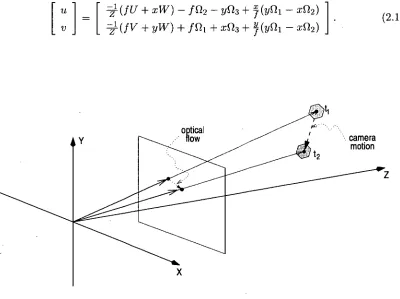
The movement of the camera in the three-dimensional domain gives rise to a movement of the irradiance pattern falling on the two-dimensional image plane. This changing brightness pattern can be thought of as the "pixels" moving. The way in which the pattern changes can be determined from the perspective projective process that maps the three-dimensional world into the two-dimensional domain of sampled still frame pictures. Optical flow is defined to be the two-dimensional motion field resulting from the projective mapping of the three-dimensional motion field, Figure 2.8. The flow components at a point in the image plane are defined as,

-=21-(fu+xw)

- fQ2 - yQ3+ 11-(yQi - xQ2)

(2.15)

Figure 2.8: The optical flow of a point is geometrically related to the

[image:37.568.73.473.402.701.2]

(38)

2.3. OPTICAL FLOW 23

Figure 2.9: Measurement of optical flow at a point is relative to the depth of the scene point. The relative velocity of a distant scene patch cannot be distinguished from that of a smaller object closer to the camera, despite the absolute difference between the velocities.

It should be noted that the rotational motion on its own is insufficient to make depth judgments, since only the translational components of the motion are dependent upon the scene depth Z. The optical flow is therefore an inverse function of scene depth, provided there is some translational motion. This phenomena is apparent when driving a car where the distant hills approach slowly, while stationary objects nearby on the side of the ride appear as if they are moving much more quickly. Eq.(2.15) is also a non-unique mapping; as evidenced by the projection of a box being identical to the projection of one twice as big and twice as far from the sensor and moving at twice the speed. Hence, objects at large distances moving quickly cannot be distinguished from closer objects moving slowly, see Figure 2.9.

(39)

2.4 Image Flow

In this thesis a distinction is drawn between the terms optical flow, which derives from the geometry of the scene and the sensor motion, and image flow. Image flow is the measured two-dimensional motion of the observed brightness pattern (image sequence) as it changes on the image plane and therefore only approximates the optical flow. Depending on their underlying assumptions different algorithms will produce different image flows.

Most current algorithms developed for accurately estimating the disparity between images rely on the following relationship holding [229],

I(x,y,t) = I(x+ox,y+ 8y, t + (5t) (2.16)

I(x,y,t) is the measured brightness of a scene point (X, Y, Z) when imaged by the camera

at the point (x,y) and for the timed position t. Likewise, /(x + Sx,y + oy,t + St) is the measured brightness of the same surface point (X, Y, Z) on the image plane for the camera at timed position t + St. If the two images are captured at different camera positions, then (Sx,Sy) is the measured two-dimensional disparity between the two images for the three-dimensional surface point (X, Y, Z).

In order for Eq.(2.16) to hold, the following assumptions based on image formation theory are required:

• Lambertian Reflectance Model

The surface reflectance properties given by the BRDF, are Lambertian. For specular reflective surfaces the measured brightness varies with the viewing az-imuth angle as shown in Eq.(2.9). As a result the requirement of Eq.(2.16) cannot be met. Lambertian reflective surfaces, on the other hand, ensure that equal energy is radiated in all directions of azimuth, see Eq.(2.10).

• Static Scene (Point Source Illumination)

(40)

2.4. IMAGE FLOW 25

Frame 1. Frame 2.

Figure 2.10: A moving light point source gives rise to an apparent motion when the true optical flow is zero.

because the point light source moves the brightness pattern on the sphere varies resulting in a non-zero image flow.

OR

• Diffuse Lighting (Extended Source Illumination)

In order to overcome the restrictive requirement of a static scene, extended light source illumination is required. The measured brightness of a Lambertian reflec-tive surface illuminated by an extended light source does not vary significantly with azimuth of the incident light rays or the azimuth of viewing, Eq.(2.11). Therefore the light reflected by a point on the scene towards the camera is unchanged by motion.

• Spatially Linear Camera Behaviour

(41)

In practice none of these requirements are met [171]. Nevertheless the fundamental

assump-tion made by all image flow algorithms is that the change observed in the image intensity is due solely to motion, i.e. that Eq.(2.16) holds exactly.

2.5 The Aperture Problem

There is a much more fundamental difficulty, than those due to a failure to meet the underlying assumptions, that must be overcome to ensure that significant deviation of the image flow from the optical flow does not occur. This difficulty is known as the aperture problem and is used to describe situations where both components of the optical flow cannot be measured [7, 9, 15]. It arises because of a fundamental information loss due to the perspective transform, and because not all pixels contribute an equal amount towards the information content of the image sequence. As an extreme example consider the case of

a spinning sphere with a Lambertian surface illuminated by either a stationary point or extended source, Figure 2.11. In this case the optical flow is non-zero. However, the sphere will "appear" to be stationary and thus has an image flow that is zero everywhere. In this example the spatial information content at the edges of the sphere is high, but the temporal information content is zero.

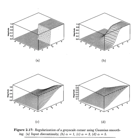
The information content of a pixel can be measured by the change of pixel value both spatially and temporally. To measure change it is necessary to consider a neighbourhood, sub-block, window, region or sub- "aperture" of the image. Windowed portions of different images are shown in Figure 2.12(a)-(d), each sub-figure illustrates a different aspect of the aperture problem.

Frame 1. Frame 2.

(42)

2.5. THE APERTURE PROBLEM

27

Frame 1. Frame 2.

(a)

Frame 1. Frame 2.

(b)

Frame 1. Frame 2.

(c)

Frame 1. Frame 2.

(d)

Figure 2.12: Instances of the aperture problem: (a) a bland field of view, (b) a stationary object, (c) an "apparent" stationary object, (d)

(43)

A major difficulty in computing image flow occurs in those regions of the image plane that are bland or lack detail, Figure 2.12(a). Consider the problem associated with observing the image plane surface through a finite aperture centred around the (x, y) pixel of a noisy sensor, shown as a dashed box. The Taylor series expansion of the image brightness pattern can be written as,

I (x + Sx, y + Sy , t + St) = I (x, y,t) + Ix(x, y,t)ox + Iy(x,y,t)Sy + It(x, y, t)6t (ox)2

+1-xx (x, y, t) + Ixy (x, y,t)8x8y + Iyy(x, y,t) (6y)2

2 2

+/(x, y, t)(5x8t ± /0 (x, y, t)SySt

+Itt(x, y, 0(602 + ...,

2 (2.17)

where subscripted variables denote partial differentiation with respect to the subscript com-puted at the point (x, y, t). If the aperture is very small, the surface is indistinguishable from a constant intensity equal to /(x, y), simply because the effects of the higher order terms in the Taylor series are much smaller than the variations due to noise. In this situation no useful information can be obtained about the motion of the surface.

If we allow the aperture to increase in size, then the contributions of the first order terms of the Taylor series eventually become larger than the noise, whereupon an overall slope is discernible above the noise. In this case we can form a single equation,

gx + 6x, y + Sy, t + St) — I(x, y, t) = Ix(x, y,t)6x + ly(x, y, t)(5y + It(x, y, Wt.

(2.18)

Provided the size of the window is large enough so that non-zero terms of the partial derivatives Ix and Iy exist, the motion term (u, v) can be estimated, where,

Sx _ U — —St ,

Sy _ V — . St

This is the first requirement in overcoming the aperture problem.

(2.19a)

(2.19b)

(44)

2.5. THE APERTURE PROBLEM 29

indeed stationary. Consequently, it could be concluded that only rapid spatial change in illuminance of the image region is required for reliable detection of image flow. The previous drawn conclusion is too imprecise, as can be demonstrated in the example shown in Figure 2.12(c). In this example the window applied to the two frames appears unchanged despite the real motion that has occurred. Furthermore, the subimage within the window is neither bland nor lacking in detail. Hence, the conclusion made above must be qualified by the statement:

"Motion can only be determined in the direction parallel to the spatial gradi-ent of the illuminance, since orthogonally to the gradigradi-ent there is little or no variation in illuminance."

This problem of only being able to determine the component of the velocity vector parallel to the gradient is another instance of the aperture problem. As a result image flow estimates often only approximate the vernier component of the optical flow, i.e. the component parallel to the optical gradient, see Figure 2.12(d).

When dealing with an aperture of this size there is only one equation to solve for two unknowns. The only solution to this difficulty is to further enlarge the size of the aperture in some way. If this is done, we can for example use changes in the spatial gradients to determine the additional conservation of gradient intensity equations,

-

= I

xx

u + Iv + I

x

t =

0,

dt

(2.20a)

and

—

d

(I)=I

x

₉

u+I v+I =0

dt

"

(2.20b)

Thus, it is evident that provided the size of the aperture is large enough that non-zero second order spatial gradients terms exist, then both velocity components can be estimated. This is the second requirement in overcoming the aperture problem.

(45)

...

• • • •

... • •

• • • •

• • •• • •

• - • H • • • • • • • • • • • • •,w- • • •

Optical Flow Field Image Flow Field

Figure 2.13: Translating along the optical axis gives rise to a diverging optical Bow field. However, the image flow field may differ significantly from the optical flow field and only at points of high curvature, such as corner points, are more reliable estimates made.

is a more accurate estimate possible. Image flow measurement techniques are therefore not only required to compute the vernier flow field, but also attempt to overcome limitations imposed by the aperture problem. The only way of achieving this is to use larger aperture sizes.

The aperture size can be further increased to improve velocity estimates, and also to allow the measurement of other geometric qualities of the optical flow field, such as the kinematics of the motion field [8]. However, as the size of the aperture is increased spatial resolution of the flow field is inevitably reduced. This is an example of the uncertainty principle;

both location and velocity cannot be estimated with infinite precision [21, 29]. Rather than

(46)

2.6. SAMPLING THEOREM FOR MOVING PICTURES 31

2.6 Sampling Theorem for Moving Pictures

The image capture process involves discretizing the continuous intensity function of the radiating scene in time and space, after it has been convolved with the point spread function of the lens system [17,21,29]. The discrete spatial units are formed from a regularly spaced array of finite sized elements referred to as pixels. Ideally, however, we take the continuous three-dimensional intensity function and multiply it with a three-dimensional impulse train to form the sampled image sequence. The purpose of the following discussion is to extend the well established one-dimensional sampling theory to three-dimensions.

Consider a one-dimensional signal f (t) and the impulse sampling train,

then the sampled signal is,

, E

8(t + nT),

n=-oo

0.

f 9(0 = f (t)

E

( (t + nT)

n=-00

E

f (nT)8(t + nT),

n=-oo

(2.21)

(2.22)

where T is the sampling period. Now, consider the affect of sampling on the Fourier spectrum of the original signal f (t). Denoting the Fourier transform pair as,

f (t) 44 F(w), (2.23)

where the Fourier spectrum F(w) is band-limited to cvm, as shown in Figure 2.14(a). The Fourier spectrum of the sampled signal is given by the transform pair,

00

f8(t) F (w) .7-

{nE

(t + nT)} . (2.24a)

The Fourier transform of the impulse sampling train is given by,

00 (5(t nT)}

E

27r

n=-oo n=-oo

where coo = 21-7- is the sampling frequency. Hence the sampled spectrum is,

(2.24b)

00 27r

(47)

(a)

F(0))

- co_m(0₀

(c)

(b)

0.3

(d)

Figure 2.14: Effect of the sampling process: (a) The original continuous signal spectrum, (b) the spectrum with sampling wo > 2w,„ (c) aliasing spectrum wo < 2wm, (d) critical sampling wo = 2wni.

and as shown in Figure 2.14(b) it consists of the periodic extension of the spectrum F(w)

where coo > 2wm . Clearly low-pass filtering to remove the periodic extensions yields the original unsampled spectrum and permits recovery of f(t). Figure 2.14(c) shows the case

for wo < 2w,i , the periodic parts of the spectrum now overlap and the original signal is now corrupted and cannot be retrieved by low-pass filtering, this is called aliasing. Figure 2.14(d) illustrates critical sampling, where Wø = Iv,. Recovery of the original signal is possible only with an ideal low-pass filter with a cutoff frequency of W m .

The minimum sampling frequency required to prevent aliasing must just exceed twice the highest frequency component in the spectrum. This minimum sampling frequency is called the Nyquist frequency or rate wN. Low-pass filtering of the continuous signal f (t) is required

before sampling to ensure the signal is bandlimited and complies with the Nyquist criteria,

LON > 2(.4.1m,• (2.25)

(48)

2.6. SAMPLING THEOREM FOR MOVING PICTURES 33

A

f(t)

-T

Figure 2.15:

2.15:

Natural or practical sampling is achieved with pulses of finite

width (7-) over a fixed interval of time T.

of finite width T, and not an infinitely long train of impulse functions, see Figure 2.15.

The finite length of the rectangular pulse train reflects that in practice sensors are finite in size. This in turn also implies that the signal is bandlimited. The Fourier series of the rectangular pulse train is,

S(t)

=

E cke

,k, k=-K

T sin(k77- /T) k_ T krT /T

Hence the Fourier transform pair for natural sampling,

f (OS (t) E ckFcw— kW13)- k=-K

(2.26a)

(2.26b)

(2.26c)

Therefore, the only difference between natural sampling and impulse sampling is; in natural sampling there are a finite number of periodic extensions, where each side-lobe of F(w) is

weighted by the diminishing Fourier series coefficients, ck, of the rectangular pulse.

There-fore if the original signal is bandlimited, and the Nyquist criteria is satisfied, aliasing will not occur.

In the multi-dimensional case the Nyquist criteria must be satisfied in each of the signal's dimensions. So in the case of a two-dimensional (x, y) signal or image, the Nyquist spatial frequency pair (kx,, ky,) must meet the criteria:

kx,„ > 2kx.„, and ky, > 2ky, , (2.27)

where (kx,n, kv,n) are the two maximum spatial frequency components in directions x and y

(49)

<=> 712 + V2 COS 0 < N

1.1

k2 k2

XN YN

frequency component the criteria is,

kx, > 2kx„,, kys > 2ky,,,, • and, wAr > avm. (2.28)

In practice the optics of a vision system bandlimit the spatial frequencies of the image, although rarely, if ever, are CCD arrays Nyquist sampled [7, 107]. This leads to mild aliasing which can often be ameliorated by post-sampling low-pass filtering or smoothing.

The fundamental assumption, on which all image flow algorithms are based, is that changes of the image intensity function in time are solely due to motion. This assumption leads to a relationship between the spatial and temporal sampling rates as a function of the motion. Fourier analysis considers the signal to be a sum of orthogonal sinusoidal components, consider one such component,

s(x, y, t) = cos (kxx + ky y + cot). (2.29a)

If the change of the image over time is due solely to motion then the sinusoid can be rewritten as,

s(x, y,t) = cos (kx (x + ut) + ky (y + vt)), (2.29b)

and therefore,

= kxtt + kyv. (2.29c)

The maximum temporal frequency is thus related to the maximum spatial frequencies by,

com = kxmfl + kym v < WN

IcxN u + ky,„v < coAr

=== VkXN 2 kYN 2

VU2

± V2 COS 0 < WN

(2.30)

where 0 is the angle between the velocity vector and the spatial sampling vector. Equation

(50)

2.7. NUMERICAL DIFFERENTIATION 35

in many applications. Techniques for effectively increasing the Nyquist velocity are required and this can be achieved in three different ways:

• Increasing the temporal sampling rate

• Decreasing the spatial sampling rate

• Increasing temporal sampling and decreasing spatial sampling

In practice image sequences are often captured at a fixed temporal rate leaving variation of the spatial sampling rate as the sole mechanism for changing the Nyquist velocity. A higher Nyquist velocity requires a reduction in the number of spatial samples, with a consequential loss in spatial resolution of the image and estimated flow field. Fortunately, through the use of multi-resolution techniques, it may be possible to obtain velocity estimates greater than the Nyquist limit for a particular resolution, a topic briefly discussed in Chapter 7.

2.7 Numerical Differentiation

As discussed in the previous section on the aperture problem, spatial and temporal gradients of the image brightness pattern are an implicit requirement in explaining the relationship between the image sequence and the image flow. Moreover, a large proportion of algorithms that make image flow estimations do so based on gradient measurements computed from the raw image data. Consequently, in this and the following section, a closer look is taken at the practical issues involved in computing image gradients.

In practice exact derivatives must be approximated by some numerical method, such as interpolation functions or finite difference approximation to the derivatives [8]. In the former approach the image intensity surface is fitted by interpolation functions for which exact derivatives exist. Classes of interpolation functions that fit this requirement include polynomial functions, and splines [96, 210, 211]. The fitting process involves determining the coefficients of the interpolation function and consequently the coefficients of the partial derivatives of the interpolation function. Therefore any errors in fitting the interpolation functions to the image surface will result in errors in the derivative estimates.

(51)

case of exact differentiation. Three options for computing finite differences exist: forward, backward and central differences. In their original work Horn and Schunck[102] used forward differences as the means of approximation. This method has the disadvantage of approx-imating the derivative at the mid-points between samples. Similarly backward differences also approximate the derivative at the mid-points between samples. Central differences, on the otherhand, approximate the derivative at sample points. This thesis presents results based on the use of central finite differences, due to their ease of understanding, speed in computing and popularity with other authors. By choosing this path direct comparisons with other works are possible, as well as with the optical flow velocities which are usually only available at pixel locations.

If we consider the Taylor series expansion about the point x of the function f (x Ax),

(Ax) „ (Ax) 3 „, (Ax) 4

f (x + x) = f (x) + Ax (x) + 21 f (x) + f (x) + 41 fw(x)

+

(Ax)5

_5! fv (x) (2.31)

then a three-point central difference evaluates the function f (x) at x, x — Ax and x x,

c_if(x — Ax) + cof (x) + cif (x + Ax) = + Co + ci)f (x) + (ci — c—i)Axt(x)

+ ci)(Ax)2r(x)

-q(ci — c_i)(Ax)3r(x)+ (2.32a)

To obtain the first order derivative approximation, one divides through by Ax and selects values for c_i, co and c1 so that the right-hand side of Eq.(2.32a) approximates 1(x). To

solve for the three unknowns, three equations are needed, which for optimality are,

0 = C1 ± Co + C-1

1 = C1 —

0 = c1 + c-1. (2.32b)

The solution is co = 0, c_i = —c1 and Ici I = 1. Hence the three-point difference mask is,

(52)

2.7. NUMERICAL DIFFERENTIATION

37 The error of this approximation is associated with the higher order derivatives,

01(Ax,3) =

3

6

-(Ax)

-

2fm(x)

+

,+-

o

(Ax)lfv(x)+...

(2.33)

Using the same process, the five-point first order difference can be specified. This yields the

optimal solution for the five-point difference mask of,

1/12 -2/3 0 2/3 -1/12

with approximation error due to higher order derivatives of,

oi(Ax, 5)

=

2 32-1 )(Axylfv(xl ( 1 2 128

-1

)(Ax

)6fvii( x

)

k

60 '

-

6171• 12 /k k k

2520' 2520 •

12 1\

Differential techniques for the accurate estimation of image flow