The analysis of structures with particular reference to elastic instability of frames

Ht

Grovt7

THE ANALYSIS OF STRUCTURES with particular reference to

Elastic Instability of

Frames

by

F. van der Woude B,E. (Hons.), Grad. I.E. Aust.

A thesis submitted for the degree of Doctor of Philosophy, in the

Faculty of Engineering,

University of Tasmania, Hobart.

[ganArkw:

p4

t444-4

w.k).

(±

)

CONTENTS

Page

PREFACE

SUMMARY. _vii

CHAPTER ONE - ELASTIC INSTABILITY OF FRAMES

1.1 Introduction

₁

1.2 The pin-ended column 2

1,3

The, practical column

4

1.4 Design techniques ₅

1.5 Design of frames ₇

1.6 Elastic instability of frames ₈

1.7 Review of existing methods for the determination of ₁₀ elastic buckling loads

• 1.8 The buckling of a.simple frame ₁₇

• 1.9 The praCtIcaIframe; experimental methods 29 1.16 The practical frame; predibted-behaviour 32

1.11 . Concluding remarks 38

References ₄₁

CHAPTER TWO - ENERGY METHODS

2.1., Introduction ₄₃

2.2 The two types of energy ₄₃

2.3 Energy analysis of a string model ₄₄ 2.4 A strain energy method applied to beams 51 2;5 Strain energy analysis of Statically indeterminate ₅₉

frames

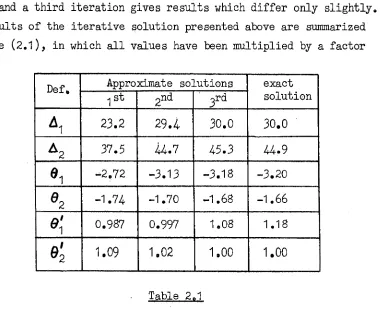
2.6 Iterative solution 60

2.7 Proof of linear combinations method 65

2.8 Physical interpretation 67

2.9 Numerical example 68

2.10 Concluding remarks 70

References 71

,•, -

CHAPTER THREE - A NEW METHOD FOR CALCULATING BUCKLING MODES AND LOADS OF FRAMES

•

3.1 Introduction 72

3:2 Development of method • 72

3.3 General analysis 74

3.4 Upper and lower bounds , 79

3.5 Physical interpretation of the linearized stiffness 82 approach

(ii)

CONTENTS (Conttd.)

Page

3.7 Two-bay Warren truss 87

3.8 Roof truss buckling in its plane

90

3.9

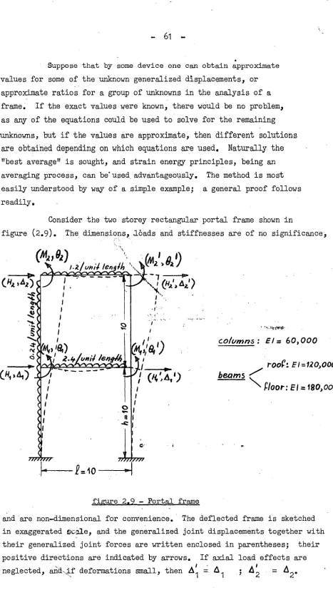
Two-Storey rectangular portal frame

97

3610

Tetrahedral frame

99

3.11 Lateral buckling of through-bridges 106 3.12 Two-bay , Warren truss through.-bridge

108

3.13

Eight-bay through-truss bridge

116

3.14 Concluding remarks

126

References

127

CHAPTER FOUR - THE BEHAVIOUR OF OVERBRACED FRAMES

4.1 Introduction 129

402 Review 130"

403 Statical indeterminacy of frames

132

4.4 The use of complementary energy in the analysis of 135 overbraced frames

405

The bending shortening of pin-ended members 138 4.6 The behaviour of pin-jointed overbraced frames 140

4.7 The measured behaviour of rigidly-jointed overbraced frames 152

4. 8 Elastic buckling loads of rigidly-jointed overbraced frames 15? 4.9 Overbraced frames with one degree of statical indeterminacy 165

4.

10

Examples of interaction

curves

166

4.11 The behaviour of initially crooked overbraced frames 173 4.12 The analysis of initially crooked overbraced frames

175

4.13 A worked example 179

4.14 The effect of prestrain

183

4.15 Concluding remarks 184

References 185

PREFACE

Broadly speaking, an engineerle constant aim is the' creation of something

which serves mankind In order to achieve his aim the*engineerjlas to tackle

numerous problems arising between the time of conception. and. the final bringing into service of the product. To this end it is convenient to picture 'the process as divided into three stages., The first Stage is to recognise the existence of the real problem, with its multitude of complexities and details, all at varying levels of importance..: The real problem is always too difficult to handle

directly, and as an'aid to thinking, great simplifications are made. The simplified problem may be called the physical model, in which only' the more important •

aspects - of -the real problem are 4efillec4 . The setting up .of a physical model

• requires skill, judgement and, in most cases, experience with similar

situations.-. It follows that the first physical model may at times be subject

to subsequent variations and revisions. Finally, a mathematical model is formulated this model attempts to describe, bymeans of mathematical equations, the behaviour of the physical model. For example, if the real problem is one of structural design, the unknowns in the final equations are usually design parameters such as stress, deflection, beam depth and so on. Thus the solution of the equations defines the behaviour of the physical model in terms of design parameters, but the degree to which these apply to the real problem depends on how well the physical model represents the real structure. Final design is achieved only after many cycles of appraisal, modifications to the physical model, refinements, re-evaluation, and so on.

The above philosophy is generally applicable, indeed it is believed to be the only successful method of problem solving in any field, especially in engineering.

This thesis is concerned with the problem of the behaviour of framed structures.. Throughout the wol-71‹ .., etphasis is placed on the geometry of the

deformations of the frame. 'Although it iS often not appreciated, the geometric • approach has dominated throughout the history' of structural engineering development.

The reason for this is obvious, because once the deformations of a structure are known, other quantities like stresses, Strains, bending moments and so on l , are easily calcUlated. Another reason is that deformations, unlike forces

(the alternative to a geometric approach is a force approach), can be pictured and drawn to Scale or sketched. Such a picture is readily obtained from

(iv)

models are quickly sketched or traced. Frequently a wire or cardboard model

may be used in order to gain a preliminary understanding of the deformations.

Once a picture of the deformations of a structure has been formed in one's mind, the formulation of physical and mathematical models follows

beld

naturally. For example, in general all the members of a frameAin two directions, twist, and stretch or shorten, but quite often only one of these types of

deformation is important. The physical model describing this type of behaviour

is obvious. Nevertheless one must not lose sight of other possible deformations;

these may need to be introduced as subsequent refinements.:

A

good example of when the first physical model must be changed, is provided by the class of frames

in which the member stretchings (or shortenings) are the primary deformations.

Such frames are liable to instability, that is the deformed frame with its members remaining straight is not always stable, and the frame buckles under certain combinations of loading. When it does, then of course the bending deformations become most important, and the physical model must be modified to include these deformations as well as the member stretchings and shortenings.

Instability of frames is One of the maintopics of this thesis.

Undoubtedly most of the ideas about instability are based on the work of

the

great mathematiciaL Leonhare Euler, in the eighteenth century. It was Euler who first established a buckling condition for a simple uniform pin-ended column. These ideas have gradually been expanded to embrace a much wider field of structures such as buckling of frames, plates, shells, beam webs, and so on. However, it should not be forgotten that Euleris analysis is only a

mathematical model of a much simplified physical model of a real column, and there is a danger of using the results of such an analysis in situations where it is no longer valid, even as a first approximation. Euler type buckling is defined by a bifurcation, or a number of bifurcations, on the load-deformation diagram for the structure; at each of these forks on the diagram the structure.

deforms according to a consistent pattern, and under constant loading it suddenly

deflects into some other pattern called the buckling mode; the corresponding

loads are called the buckling or critical loads. This type of buckling is in fact a reasonable description of the behaviour of isolated columns and statically determinate frames, but in most other structures there exist influences which do. not permit them to deflect under constant load, and their buckling behaviour cannot therefore be of the Euler type. Examples of this different buckling

(v)

In addition, there is the question of the practical significance of the existence of some unstable state. In practice a structure always

exhibits deformations other than those which are considered in the physical

model. Among these are the deformations, which arise when the structure

buckles, and their importance usually increases as the strUbture is subjected to greater primary deformations. :

When the additional deformations

are

included in the analysis, the calculated load carrying capacity of the structure is greatly affected, and may be far less than the buckling load predicted if they are ignored.

Unfortunately, some of the above considerations are frequently neglected in current literature. Thus, although the problem of structural behaviour has

been intensively

investigated, there remains an untold number of questions.

The author hopes that the work to follow herein may provide a useful attempt to pose important practical questions, and give a guide as to' how they may be answered, and hence promote a clearer understanding of the behaviour of

structures, which is urgently needed by structural

designers.-

In conformity with the definition of an engineer's aim, as given

earlier, the aim of this thesis is to investigate the problem of the behaviour of framed structures, with particular reference to elastic instability.

Design is continually kept in mind as being the end product of this research, and wherever possible, design procedures are suggested. Some of these may not be unique, nor have they been proved in practice, but the author believes that the principles are soundly based on a reasonable understanding of

ACKNOWLEDGEMENTS

In a work of this kind it is impossible to acknowledge each and every person who at some time or other has been involved in its fulfilment. I hereby thank everyone conoerned, and in particular I wish to express my deep

appreciation of the helpful advice and stimulus received from the following

persons:

Professor A.R. Oliver, Professor of civil and mechanical engineering at the University.of Tasmania;

Dr. M.S. Gregory, Reader in civil and mechanical engineering at the

University of Tasmania, and supervisor of this research;

the late Professor W. Merchant of the Manchester college of science

and technology, England;

emeritus Professor J.J. Koch of Delft, Holland,

Thanks are also due to Miss A. Clark for the care with which she prepared this manuscript.

The work described in this thesis was carried out during the period March 1963 to December 1967, in the department of civil and mechanical

engineering at the university of Tasmania, Hobart Australia.

I hereby declare that, except as stated herein this thesis contains

no material which has been ac:epted for the award of any degree or'diploma

in any university, and that, to the best of my knowledge or belief, this thesis contains no copy or paraphrase of material previously published or written by another person, except where due reference is made in the text

of this thesis.

(vii)

SUMMARY

CHAPTER ONE begins with a preliminary examination of the" problem of instability of frames. This is followed by a brief description of the development of instability studies, starting with Eulerlb analysis of a pin-ended column and culminating with the now classical matrix analysis of rigidly jointed frames. A simple frame is analyzed in.order to show that the various methods of analysis all have the same physical and

mathematical models but employ different methods of handling the mathematics.

Experimental methods are discussed, and the chapter concludes with the

formulation of a mathematical model suitable for the prediction Of frame behaviour. This model can be used to obtain an estimate of the load carrying of a frame, and hence it provides a useful design procedure.

CHAPTER TWO deals With the application of energy methods in structural analysis. The two types, Complementary energy and strain energy, are introduced by

means of a simple example and it is clearly shown that they are equivalent to geoMetric and statical considerations respectively. :These ideas are

extended and applied to some common beam problems, for which rapid approximate solutions are found. It is then shown that the classical matrix method of structural analysis, using joint displacements as unknowns, is equivalent to a strain energy approach, and this naturally leads to .S. powerful

approximate method of solution. The method is applied to the analysis of a two-bay eight-storey building frame; and the results are compared with a computer solution.

CHAPTER THREE proposes a new method for. the determination of buckling modes and loads of rigidly jointed frames.' The method is based on a strain energy analysis, and it is identified as a.linearization of the .usual stiffness matrix approach. This leads to a useful iterative numerical scheme. Proofs are given of Upper and lower bound theorems, and the method is applied to a number of frames, including a few in thr6e dimensions. Most of these

analyses are checked by 'experimental measurements.

.CHAPTER FOUR _{extends the work into the analysis of redundant frames. The}

complementary energy method is proposed as the most convenient way of deriving the compatibility equations relating the member shortenings. A mathematical model is developed for the evaluation of the shortening of

bent pin-ended members. The problem of buckling Of redundant frames is introduced by means of an analysis of a 'simple pin-jointed frame, and

of the results of experimental work on the behaviour of redundant frames with rigid joints. It is shown that the buckling behaviour is not of the Euler

type. An earlier definition of instability is therefore closely re-examined,

and this leads to a new formulation of the problem. A general stability

criterion is set up mathematically and applied to some simple singly-redundant frames, and the results are compared with measurements. In conclusion a

NOTATION

Symbols are defined when they first appear in the text. The general

notation used is as follows;

A

cross sectional area complementary energy Young's modulus f(or0r) stress

torsion modulus

second moment of area (or unit matrix) polar secon4 moment of area

at

stiffness matrix

member length

bending moment

axial force in a member

• 4

Euler load of pin-ended member r = Eia radiu$ of gyration

strain energy applied load X generalized force

generalized displacement (or coordinate)

y(or z) deflection

A

member shortening (also sway)

strain

eP curvature A latent root

to rotation

- 1 -.

CHAPTER ONE

ELASTIC INSTABILITY OF FRAMES

1.1 INTRODUCTION

Instability of structures is a subject which has received a considerable amount of attention, originating with Buie/ 0 s analysis of the buckling of a pin-ended column, The classical approach developed by Euler also forms the foundation of the analysis of instability of structures. A structure is said to be in stable equilibrium when small

changes in loading are accompanied by correspondingly small changes in

the deformations. On the other hand, instability is associated with a

state of unstable equilibrium when small changes in loading produce large changes in the deformations ultimately resulting in failure of the structure. Mathematically this definition of instability can be

written as

ay/aX (1.1)

where x is a generalized displacement and X is the corresponding generalized force. Inversely this becomes

ax/ax = 0 (1.2)

and this formal definition of instability is adopted in the work to follow; in practice it is easier to use than the former, which exhibits the difficulties of manipulating infinities.

Broadly speaking failure of a structure by instability may be separated into two distinct classes. Firstly there is the failure brought about by large scale yielding of parts of the structure. When this occurs

these parts continue to deform under constant or nearly constant load and may be thought of as hinges. As more hinges form the structure eventually becomes a mechanism and collapses as such, the load at which this occurs is known as the collapse load; the analysis of this type of instability

is a complete study in its own right.

Secondly, large deformations may take place in the elastic range of the material, if at some stage the structure can no longer support its loads due to its decreasing stiffness as the loads are increased. This type of instability is usually referred to as elastic buckling.

Essentially this problem is the same as that posed by Euler, and in order to obtain a clear understanding.of what is involved, the fundamental ideas are recapitulated in the following sections. The treatment given in these sections is found in most textbooks on structural analysis but is included here for the sake of completeness.

1.2 THE PIN-ENDED COLUMN

Consider a pin-ended column AB initially straight, compressed by an axial force P as shown in figure 1.1. We ask ourselves if there exists

8

figure 1.1 - Din-ended column

an equilibrium configuration other than the straight form. Supposing there

is, let y = f(x) describe this configuration. Then the bending moment at the point (x, y) on the deflected centre line of the column is given by

m =

-

py

_(1.3)

anticlockwise moments being considered positive. If the deflections y are small compared with the length of the column, the curvature is approximately given by

T =

d2 y/dx2

(1.4)

According to the usual assumptions in linear theory of bending of beams, the

bending moment is related to the curvature by the expression

M = EIO _(1.5)

Thus equation (1.3) becomes

EI(d2y/dx2 ) + By = 0

(1.6)

The solution of this differential equation is

Use of the boundary conditions of zero end deflections reduces this to

y = a

n sin kn x (1.8)

where k

n = ni1/1 ; n = 1 2, 3, . . .

or y = 0 everywhere, this solution being trivial. It is seen that a deflected equilibrium configuration is possible only for certain discrete

values of P given by

P

n

= n

2

_ir

2

EI/12

and the corresponding deflected shapes are of sinusoidal form y = a sin(n175ç/1)

n n

(1.9)

1.10)

where an is undefined as to magnitude, although it is restricted by the

approximate expression for the curvature and by the condition of linearity implied in equation (1.5).

P

n

is called the nth. buckling load of the

column and yn is called the corresponding buckling mode.

. This problem was first solved by Euler . some two hundred years ago and is still used today as the basis of all elastic instability studies' relating to frames. When n = 1 we have what is called the fundamental buckling condition, and P

i

=1EI/1 2 = Q

is commonly known.as the Euler

load s his being

the smallest load at which the pin—ended column has an

equilibrium configuration other than the straight form. For values of P

less than Q the column is in equilibrium only in the straight form, at

•

P = Q the column is in neutral equilibrium, and at values of P greater than

Q

the column is in unstable equilibrium. The

behaviour

of this mathematical

model of the column is indicated graphically in figure.(1.2) by two straight lines.

LOAD

(p) _{a., s in(irx/E)}

DEFLECTION ( )

The buckling loads and modes for columns with other end conditions can be obtained by similar analyses, and in general it is possible to put the fundamental buckling load in the form

P₁ =1r2EI(e1) 2

where (el) is called the effective length of the column,. that is the length

of a pin-ended column having the same buckling load as the column under question.

1.3 THE PRACTICAL COLUMN

EulerLs.analysis, as set out in the previous section, is idealized in

the sense that it implies perfect straightness of the column, ends completely

free to .rotate, purely axial load (that is no eccentricity), uniformity of

cross-section and homogeneity of the material. In practice such conditions are never realized, and the lack of these conditions is broadly classified under the heading of. initial imperfections..As a consequence of initial imperfections, a column under test will begin to deflect as soon as a load

is applied and Euleris analysis is therefore no longer a reasonable

representation of the behaviour of a practical column. The mathematical analysis can be improved to take into account some initial imperfections.

such as eccentricity of loading, initial curvature and the effects of end

moments,. and experiments have shown that for a large class of columns the

behaviour under load can be fairly well predicted. If the ends of the

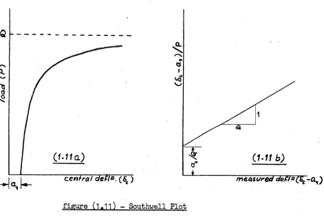
column are pinned, (that is free to rotate,) it can be shown that as the ratio P/Q approaches unity the behaviour of an imperfect column is

asymptotic to Euler's theory. This has led to the very useful experimental technique known as the Southwell plot, which is discussed in more detail in section (1.9). The Euler load is generally not reached in tests, unless there are some external restraints) since as the deflections tend to become large the strain in parts of the column exceeds the yield value.. How closely

the Euler load can be approached depends on the magnitude of the imperfections.

Despite the fact that the Euler load may not be reached in practice, it is

and remains a useful result. The behaviour of a column under test is shown

superimposed on the Euler mathematical model in figure (1.2). The various

curves are for different magnitudes of initial crookedness and the post-yield

\ _{Proper/lona/ limh€}

Co

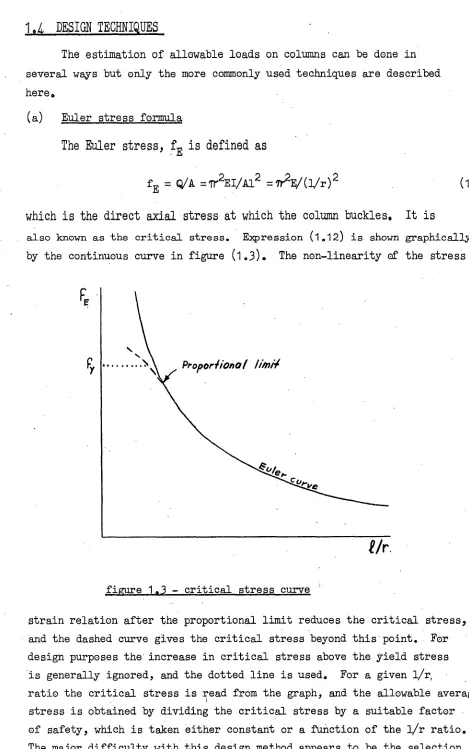
1.4 DESIGN TECHNIQUES

The estimation of allowable loads on columns can be done in several ways but only the more commonly used techniques are described here.

(a) Euler stress formula

The Euler stress, f

E

is defined as

f

E = OVA =1r2EI/Al2 =V2E/(l/r) 2 (1.12)

which is the

direct axial stress at which the column buckles. It is

also known as the critical stress. Expression (1.12) is shown graphically by the continuous curve in figure (1.3). The non-linearity of the stress

F

E

[image:15.542.36.505.98.847.2]

Ur

figure 1.3 - critical stress curve

strain relation after the proportional limit reduces the critical stress, and the dashed curve gives the critical stress beyond this point. For design purposes the increase in critical stress above the yield stress

is generally ignored, and the dotted line is used. For a given l/r,

(b) Design based on initial imperfections

In this design technique the effects of initial imperfections are all replaced by a single initial curvature pattern. The function representing this pattern does not affect the calculations to any significant extent, and for simplicity a sine curve is generally used, that is the initial shape of the column is defined by

yo = ao sin(iTx/1)

(1.13)

If y is the shape of the column when it carried an axial load P I then

equations (1.3) and (1.4) still hold, but the bending moment-curvature

relation is changed to

EI(1)-10 )

(1.14)

where 00 is the initial curvature. The differential equation is solved in

the usual way, and the maximum extreme fibre stress occurring at the centre

of the column is readily found to be

1

f

max

=

(P/A)[1 + A a0/(17P/Q)Z] (1.15)

where A is the cross sectional area and Z. is the section modulus'. Equating

this to the yield stress, we obtain the well known

Perry

formula

ft = PI/A = -efy + (n+l)fE] .4- 1/[fy+ (n+1)fE3 2

—4

fy fE. (1.16)

where PI is the load which will just cause first yield f in the extreme

fibres, and f E is the Euler stress as defined above. The quantity n is

a measure of the magnitude of the imperfections and is defined by

n = a 0 v/r

2

(1.17)

where v is the distance from the neutral axis to the extreme fibres, and r is the radius of gyration. n is usually specified as some fraction of the hr ratio, which is meant to allow for small inherent eccentricities as well as initial curvature. The allowable average stress is obtained by dividing fl by a factor of safety.

(c) Empirical Formulas

7

(i) the Rankine formula, f = a/A+ b(l/r) 2]

(ii) the Johnson parabolic formula, f = a - b(l/r) 2 (jai) the straight line formula, f = a - b(l/r)

In all

cases f is the allowable average axial stress, and the constants

a and b are chosen to fit experimental results. A factor of safety is

also incorporated in these formulas. The use of these formulas is generally restricted to certain ranges of the 1/r ratio.

*

There are of course numerous arguments for or against the use

of any particular design tecnaique. Present day design codes differ in opinion, but with sensibly chosen numerical values in the relevant

formulas there is probably little difference in the end result, irrespective of which technique is used. It must be borne in mind that all the design formulas mentioned are in reality empirical,as each involves the selection of a factor of safety or other quantity, and these are obtained only by

experiment and by experience of what has been proved to be safe. This

is the basis of all design codes.

If the column has end conditions other than pinned, the length 1 in the design formulas is replaced by the effective length.

1.5 DESIGN OF FRAMES

So far the discussion of design methods has been restricted to isolated columns whose effective lengths are known or can be readily estimated. In the design of compression members of frames these design

formulas are

still applicable,

provided the effective lengths of these

members can be found. Since the end conditions are generally not known beforehand Some difficulty arises, and this is the real problem in frame design. De -Sign codes usually give a table of effective lengths for compression members with various end connections, but, although these are reliable, the designs are probably overconservative since attention

individual basis should be adequate. However, most frames have rigid or nearly rigid joints, so that lateral deflections in any member affect the whole frame. The magnitude of the deflections depends on the stiffnesses of the joinbJ, which in turn depends on the conditions in the neighbouring members, and so on. Thus the concept of a buckling member is no longer useful, and the stability of the whole frame must be investigated and used

in design, together with an overall factor of safety.

Although it is possible to calculate the elastic buckling loads of frames, and hence the effective lengths, more numerical computation is required than is generally warranted for routine design office work, and therefore most frames are designed using empirical information from design

codes, Here again the only justification seems to be the satisfactory

performance of past designs. The designer is also faced with the question of economy; that is, the additional cost of non-standard

member sizes,

which may have to be used, could well exceed the savings on the "more efficient" design.

The problem of frame design is discussed

again in section

1.11),

together with the author's proposal for improved design techniques.

1.6 ELASTIC INSTABILITY OF FRAMES

As

for

the pin-ended ColUMni the basic

problem of

elastic

instability of frames is to find those loads, or combination of loads, fot.which.the frame has an equilibrium configuration other than that in

which all

members remain straight. If the frame has pinned joints, the

buckling load Would be the smallest load at which one of the members carries its Eulet load, for then this member buckles on its own and cannot sustain an increase in load, thereby effectively rendering the frame a mechanism. If the frame is m ,-fold statically indeterminate with respect to the axial forces In its members, then in general (m + 1) Members Must carry the Eider

load when

the

frame buckles. For

the time being, only

statically determinate frames are considered; the buckling of redundant frames is treated in chapter four. The buckling mode in the statically determinate case i8

defined

Simply by the deflected shape of the buckled member, that is

a

half sine wale.

a manageable mathematical model. These are common to all methods of attack and are described here in order to keep in mind the limitations of the analyses. For simplicity, only plane frames buckling in their plane are considered, but the arguments are readily extended into three

dimensions.

The first simplifying step is to replace the real frame by a physical model of the same dimensions, having its members perfectly straight initially, the centrelines of the members lie in one plane

and intersect at the joints, the joints are perfectly rigid, and

loads are applied at the joints only and in the plane of the frame .. It is also customary to neglect secondary bending moments arising from changes in the geometry of the frame due to the changes in the axial lengths of the members. The bending moments resulting from lateral

deformation of the members are called primary bending moments.. It

is clear that the, simplified model of the frame can be loaded so that

the members remain straight. To define buckling of the physical model, the concept of an initial disturbance is useful. Suppose the frame is given a disturbance, exciting lateral deformations in the plane of the frame; if there is no other load on the frame it remains in stable equilibrium, and the deflected shape can be calculated by standard methods of analysis. If the disturbance is applied When the frame carries some load, additional bending moments arise as a result. of the axial forces in the members, and hence the deflections are increased, giving increased bending moments and so on. Equilibrium may be stable or unstable depending on the magnitude of the primary load. Obviously if this is small, equilibrium is stable but at'

some discrete

values of the primary load the additional deflections

due to the axial forces in the members are just larger than those

caused by the disturbance acting alone, and then the final deformations are undefined and the frame is said to buckle. Although the,

magnitude of the deformations is undefined, the frame assumes a definite shape, called the buckling mode In general there exist several buckling modes, each associated with a different value of the primary load. In this definition of buckling it has been assumed that although the deformations are undefined as to magnitude, they are sufficiently small not to cause yielding, and that the usual small deflection theory is applicable.

The basic problem of elastic instability is therefore the

determination of loadings on the physical model for which an infinitesimal disturbance is sufficient to excite buckling. In actual frames,

- 10

eccentricity of loads and many other factors cause the members to deflect as soon as load is applied,in the same way as the pin-ended column in section (1.3). The behaviour of practical frames is discussed in more detail in sections (1.9) and (1.10).

Several methods of solution are available; the more commonly

used approaches are summarized in the following section, in a sequence

designed to bring out the ideas leading up to the new method developed by the author in chapter three of this thesis.

1.7 REVIEW OF EXISTING METHODS FOR THE DETERMINATION OF ELASTIC BUCKLING LOADS

(a)

Moment distribution.convergence as a stability criterion.

This method

is

due to Hoff (reference 1), and is the result of the impact of the Hardy-Cross moment distribution method on structural analysis. A disturbing moment is applied at one joint of the frame, and the frame's response is determined by moment distribution. Hoff originally

used the Berry functions

(00),

tabulated by Niles and Newell (reference 2),

to calculate the stiffness and carry over factors of the members, but more recently these have been tabulated directly by Live sley and Chandler

(reference 3).

At loads below the

critical, the

moment distribution

process converges, whereas at loads above the critical value the process

diverges. The convergence

of the moment

distribution process is therefore

a useful criterion of stability. If only a single

disturbance is used, it

is necessary to ensure that it does in fact excite a component of the buckling mode under consideration. In actual problems it is likely that the designer will want to take into account the initial curvatures in the members, lateral loading of the members and other effects, so that a disturbing moment is not needed to induce primary bending. This is perhaps the main advantage

oEtbe:11,41T:method _- in that the primary bending moments and a check on the

stability 'are obtained by one computational process, although the nearness of the buckling load will in general not be established unless these

calculations are repeated for other load values.

On the other hand there are several major disadvantages to

this

method. Firstly, in some cases it is difficult to establish whether the distribution process is converging or. diverging. This can partly be overcome by changing the order of balancing the joints. Secondly, even if the buckling load is sandwiched closely, the method does not give the associated buckling mode directly, this must be computed separately.

— 11

by extrapolation or interpolation. Finally, the Hoff method involves

a considerable amount of numerical labour ) as in any practical frame

it takes a long time for a disturbance at one joint to be distributed throughout the frame and even longer for the carry..overs to return to that joint.

Gregory (reference 4) has shown that the amount of

qomputation is considerably reduced by applying disturbing moments at

all the joints rather than at only one joint. This is particularly so

if the correct buckling mode can be pictured, for then the disturbances can be given the correct signs and ratios so as to excite the required buckling mode; model observations are almost always necessary to

provide this picture. It is seen that this technique is very similar

to that of taking into account the initial curvatures of the members. If the initial curvatures are chosen, on the basis of model tests or otherwise, to closely represent the final buckling mode, then the final bending moments will be very reliable for design purposes, and convergence (or divergence) of the distribution

Procdis

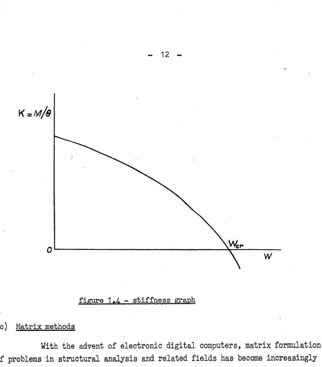
should be rapid.

(b) Stiffness method

Merchant (reference 5) developed a method which determines the moment M requited at a particular joint of the frame to produce a

given rotation 6 at that joint. The stiffness K s defined by

M = Ke (1.18)

is calculated for a number of load values, and the lowest buckling load is that for which the stiffness first becomes zero. Although moment distribution is used in the numerical work, this method has the advantage of giving a graph such as in figure (1.4), and most of the difficulties mentioned in part (a) of this section do not

exist, because we are now searching for a zero rather than an infinity. Nevertheless, Several distribution processes must be carried out to

[image:22.542.41.506.27.557.2]

12

figure 104 ,,_atiffness .graph

(c) Matrix methods

With the advent of electronic digital computers, matrix formulation

of problems in structural analysis and related fields has become increasingly

popular, Matrix methods are particularly suited to the problem of the

determination of elastic buckling loads and modes of framed structures.

When the matrix of the equations relating member end moments to the corresponding end slopes is set up s the mathematical criterion for buckling is that the determinant of coefficients of M orovanishes.

Essentially this is a generalization of Merchant's stiffness method; all the joints are rotated and the requirements of joint equilibrium

give the joint moments necessary to produce these rotations. The stiffness s and carry over factor c) as tabulated by Livesley and Chandler ) (see also

appendix A) relate the end moments to the end slopes by the equations

MAE = k(seA + sc%)

(1.19) MEA = k(sC0A+ s 9B)

where k = EI/li and the first subscript denotes the en 0 under consideration..

• For a plane frame consisting of say n joints, equations such as (1.19) are

13

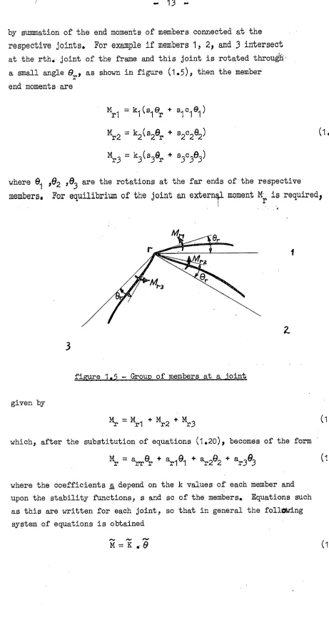
by summation of the end moments of members connected at

the

respective joints. For example if members 1,

2 ) and 3

intersect

at the rth. joint of the frame and this joint is rotated through a small angle

er

as shown in figure (1.5)2 then the member

end moments are

m

r1 = 1,c1 (

81

er "1

e

l )

M

r2 = k2 (5261r

82c2 612 )

Mr3

= k3 (s 3611, s3 c3603 )

(1.20)

where

6

_{1 )}

₁₉₂

_2'

6

3

are the rotations at the far ends of the respective

members. For equilibrium of the joint an external moment 111,

is required )

3

figure 1.1= Group of members at a joint

given by

M

r =M r1 +M r2 +

M

(1.21)

which, after the substitution of equations (1.20) becomes of the form M=a 0

r +ar 01 +ar2

02

+ a

r3

e3

(1.22)

r

rr

l

where the

coefficients a depend on the k values of each member and upon the stability functions, s and sc of the members. Equations such

as this are written for each joint, so that in general the follOwing system of equations is obtained

[image:23.542.49.510.79.948.2]

14 —

where K is a symmetric matrix, called the stiffness matrix, the elements of which are a function of the stability functions of some or of all the members

of the frame, M is the vector defining the joint moments, and 9is the vector

defining the corresponding joint rotations.

In general the mathematical model of the frame is undisturbed, so that M is a null vector, and equation (1.23) becomes

= (1.24)

A non—trivial solution exists only if the determinant of K : that is IKI

_{s is} identically zero and then the rotations are undefined in magnitude, but they bear a definite ratio to each other.

Thus ) mathematically speaking, the problem has been reduced to the determination

of thoseload values for which IK I vanishes, and this is

perhaps the most powerful method for the estimation of buckling loads and

modes of framed structures. Here again several mathematical techniques are available ) but it suffices to describe only the more commonly used methods of

solution.

(i) Evaluation of the determinant

The

classical approach in this case is the obvious one, that is

to evaluate the determinant at a number of load values. The buckling loads are then found graphically and the associated modes are calculated by setting an arbitrary rotation equal to unity and solving the equations for the

remaining unknowns. For frames of any complexity the order of the determinant becomes high ) and this method is apt to become very tedious as well as

inaccurate due to accumulating errors in the evaluation of the determinant.

(ii) Latent roots of the stiffness matrix

Gregory (reference 6) has shown that equation (1.23) is conveniently

p.-

solved by the

extraction

of latent roots and latent vectors of the matrix K.

A latent rooti

A ,

of Zis defined as

A = m

_{i/ei =} 2, 0 • ) n (1.25)

From this definition it is seen that

A

represents a kind of generalised overall stiffness of the frame. Substitution of equation (1.25) into

(1.23) yields

• 15

where I is the unit matrix. That is, the matrix

#.

1Z

.

is modified by

subtracting

A

from each of the elements on the leading diagonal. As before, a non—trivial solution exists only if the determinant

ri —All is identically zero, which is the condition used to calculate

A .

In general there exist n latent roots for a given (n x n) symmetric matrix )

each associated with a different latent vector.

At

any of the buckling loads of the frame the determinant

R

I

itself vanishes, and the righthandside of equation (1.23) is zero s so that one of the latent roots of the matrix K also vanishes. It can be shown that at loads smaller than the lowest buckling load all the latent roots are positive, whence it follows that the lowest buckling load is that for which the smallest latent root first becomes zero, and the associated buckling mode is the corresponding latent vector. The

largest

latent

root of a matrix is readily extracted by a standard

intensification process (see for example reference 7), and Gregory shows that this can be used to find the smallest latent root by what

he calls a "parallel shift" of the latent roots, which is

analogous

)1

to a transfer of origin, That is, if is the largest latent root of the matrix (R. — then the smallest latent root of K, A l is given by

A

₁

_{. +}

g 316

and the lowest buckling load is found by graphing k i against load

to determine its first zero..

(1.27)

The most important feature of Gregory's method is that

the parallel shift does not change the latent vectors of K; hence the latent vector associated with the largest latent root of (I— gI) at the lowest buckling load is in fact the corresponding buckling mode. A further advantage of this method is that convergence of the

intensification process is greatly enhanced by starting with a trial vector close to the buckling mode, and this can be obtained from tests on crude models of the frame, often a cardboard model is sufficient.

Although it may seem that the extraction of two latent roots is required, the labour involved is but a little more than that of extracting one l because only a rough estimate of g is required; it is necessary only to ensure that the shift is numerically larger than the mean 'of

A

₁

and g.

16 -

(iii) McMinn's method

McMinn (reference 8) calculates the lowest buckling load from the applied matrix Q defined by

^-_1

Q = BD .i (1.28)

where BD is the matrix obtained from K by dividing each column by its element on the leading diagonal, and the elements on the leading diagonal are zero.

The lowest buckling load in this case is the load at which the

largest latent root of 'lequals -2. Although McMinn's modification of the

stiffness matrix requires less work than Gregory's parallel shift, it suffers the disadvantage that the latent vector of 1 76 cd2responding to its largest latent root is not simply related to the buckling mode; the mode must be

computed separately. This also necessitates the use of an unguided choice

for the first trial vector in the intensification process.

(d) Energy methods

Rayleigh (reference 9) first conceived the idea of using assumed deflection curves in a strain energy integral, and minimizing this integral to calculate what he calls the "disposable parameters" involved in defining the curves. This method of approximate solution is used to solve a wide variety of problems; for example the buckling load of a pin-ended column may be calculated to any degree of accuracy by continually improving the

assumption for the deflected shape (see for example reference 10).

The Rayleigh method is readily extended to the stability analysis of frames. The buckled shape of each member is guessed, its strain energy is evaluated, and the results are summed to obtain the total strain energy of the frame. The strain energy of a single member, U is defined by (see chapter two)

t

a 0 G_s

A

jrtild0dx iM de

A

-IMB

AB A -Id (1.29)

0 0 0 _{0 0}

where Ms the axial shortening due to bending and is given by

A =

(ay/dx>

2

dx 0

In the case of a linear moment curvature relation, the first term in equation (11.29) becomes

E

f

Imdfdx =

ifE4d+dr,. Eite dx = jEI(d2y/dx2 )

ax

o o

(1.30)

17 —

If the loaded but undeflected state is chosen as energy reference

datum, then under the assumption already made that P remains unaltered by the lateral deformations, the second term becomes

P d=

.4-Pjr(dy/dx) dx %2

0 0

(1.32)

For the whole frame, the total

strain energy is

a ii t t. 6;4

es

u

=

MVO rs 0

{-i- j

E I ( d 2y/ d x2 ) 2 dx .--IPS (dy/dx) 2dx

—IM

d 9

-INA

d6.

0

(1033)

o 0 AB

It is seen that the first term in this summatiOn represents the internal strain energy of bending for the whole frame. The second term is the work done by the external loads on the frame, and it is readily shown that

all 8.

If

P ,1 (4y/dx)2dx

r

i = i Wi d6i

mern erS

where g i is the deflection of the load W i y and the summation extends over all the

applied loads. Similarly, the summation involving

the member end moments is equivalent to

19;

(1.34)

(

1

.35)

whichistheworkdonebythejointmomentslCby rotating the joints 0

through the small angles

e. ,

the summation extending over all the joints. In the general analysis of the idealized mathematical model, the joints are undisturbed, and this term therefore vanishes. It remains then to specify the deflected shape of each member in terms of one parameter, or more in the Rayleigh—Ritz method, evaluate the necessary integrals, and minimize expression (1.33) with respect to the disposable parameters. This leads to a system of linear equations, and hence to the usual criterion that the determinant of coefficients must vanish for a non—zero solution of the parameters.

1 ..8 THE BUCKLING OF A SIMPLE FRAME

In order to obtain a deeper appreciation of the underlying principles in the analysis of elastic stability of frames, the

(b) Symmefric

mode

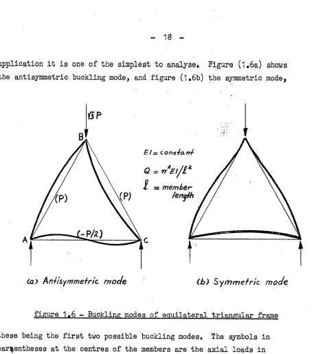
= 18

application it is one of the simplest to analyse. Figure (1.6a) shows

• the antisymmetric buckling mode, and figure (1.6b) the symmetric mode,

41111111111

1

1

1

111

1

11111k

E = con5kLm4

Q fr2EVP = member /enyfh

•

[image:28.542.32.492.44.559.2]

co.) Aniisymmelric mode

figure 1.6 = Buckling modes of equilateral triangular frame

these being the first two possible buckling modes. The symbols in parentheses at the centres of the members are the axial loads in the members, compression being considered positive. In this problem

it is convenient to treat

P

as the primary load parameter, and the

lowest buckling load is denoted by

Preliminary analysis

Obviously the compresion members AB and BC have some restraint against rotation at the ends, so that P er must be greater than

ta,

the Euler load of the members. Also, in the case of symmetric buckling, these members are equivalent to columns built—in at B, and

partially restrained at A and C. If A and C were free to rotate, the buckling load would be 2.05Q, which is therefore a lower bound for

symmetric buckling. For the anti—symmetric mode, _MBA=

MBC= 0,

SO

4.

6

19

This preliminary analysis establishes that the fundamental

buckling mode is antisymmetrical, and that P ar lies between

Q

and 2,05Q.

(a) Solution by the moment distribution convergence criterion

Figure (1.7) shows the distribution and carry-over factors of the members, at the primary load P = Q. A disturbing moment of 100 units is applied at joint B, and the distribution process is carried out in the table alongside figure (1.7), only half the calculations being

449= /₀₀

MAC C4

-32.5

-13.0

8.4

3.4

-2.1

- 0.8

50

—17-5-

-1• 3

4.4

41

84,0c

M9=2.8 0. 3

0.2.

-0-/

TOTALS 36.0 - 3'.0 3.o

FINAL MOMENTS SO. 0 - 50. $0.0

figure 1,7 - distribution and carry-over factors

shown as they are antisymmetrical. It is seen that after joint A is balanced, and therefore also joint C I there is an out of balance moment of 28 units at joint B p and since this is less than the original disturbing moment of 100 units, the process is converging, so that P er has not been

exceeded, as was to be expected from the preliminary analysis. The out of balance moment of 28 units, when redistributed, obviously gives identical

calculations decreased by the ratio 28/100, so that the final bending

o.9

,

73

- 20 -

The distribution process is repeated for a primary load of 2Q in the following table, and in this case one cyole is sufficient to indicate

divergence

)

so that P

er

has been exceeded.

Mit= 100

A44111 . MAC , /148A

1235 SO

- 33 -1202 -824

_ 3_91t

II 33 R 6 2

Kizowing values of P both above and below P er we can halve the interval between converging and diverging cases, thereby successively reducing the range until the desired accuracy is obtained. It is found, after four more distribution processes, that the buckling load is within the range

1.60Q < P er .< 1.65Q

and for all practical purposes we can

take P

er

= 1 63Q.

As mentioned earlier, the buckling mode is not obtained and must be computed separately. The best way to do this is to work from the bending moments calculated at a'load somewhat less than P er. At

P

= 1.6Q the bending moments are

MBA = M.Bc = 50 units M = -M

AC = 1145 units = -MCA = MOB AB

The joint rotations are given by the equations (EI/1)6A =

[2

1

2M

AB

-4(11

BA

(EI/1)09/3 = _[-'NMAB

₄

_14BA)

where 0( ,

p

are the Berry functions for member AB. Dropping the factor (6E1/1), and using the tables in Niles and Newell, we obtain

=

.1040 ;G B = 2470

As a check the calculations for member AC give

modified dish-ILI/lion fociors

- 21

Hence the buckling mode is approximately expressed by the ratio

6

A

:0

B

:

C

i."0

.376

It can be seen that for a frame having several joints, considerable

extra computation is

needed to obtain the buckling mode. In this

particular problem convergence or divergence is readily detected, but in more difficult frames this is not always the case, and it is usually necessary to perform additional tests such as altering the order of balancing the joints. This is especially important

if the fundamental mode is not known. For example, if equal and opposite disturbing moments are applied to joints A and C of the equilateral

triangular frame ) the symmetric mode is excited, and if the distribution is kept symmetrical it will be found to be convergent at loads greater

than

1.63Q. Altering

the order of balancing in this

case reveals

divergence, indicating that the fundame461 buckling load has been exceeded.

(b) Solution by Merchantls stiffness method

In this method joint B is rotated a unit amount, and its

stiffness

calculated, that is the moment at that joint. This is most

easily carried out in the form of a relaxation table. Since individual'

member end moments are not of interest, it is convenient to use the so

called modified distribution factors, that is if an external moment M

is applied at a jointi then the moments required at neighbouring joints

to prevent their rotation are found by multiplying M by the appropriate modified distribution factors. These are shown alongside the relaxation table below. The first line in the table gives the moment required at

RELAXATION TABLE Opera lion .

61

A

41_

6.517

&sit-1601Am

2.19

2./q

4o/once

-2417 -2.1

alislk _{-0.36 -1.26} -0-56

bal. o- s6 o-s6

clis-f-

0. /# 0.32 0./4

ba I -O./4t -0-14 oh's/. -o.oit -o.og -0.09 44 1

dia.

0, oil,

0.0/ 0-02

0.04

0.0/ einal

5. 0

3.0

2.0

1.0

0

22 —

joint B to produce a unit rotation there. This is distributed in line

(2), and at this stage

e

B

=

1 ;

e

A

=e

c

=

O. The moments at A and C are then balanced by equal and opposite external moments there, which in turn must be distributed, resulting in unbalance of A and C. These are again balanced and distributed, and so on until the out of balance moments are

sufficiently small. Equations (1.19) are used to calculate the end moments, and the primary load is arbitrarily taken as 045Q* To the accuracy shown, the joint stiffness at P = 04,5Q

_{is 5.59.}

Similar calculations at other load values give the stiffness plot shown in figure (1.8). from the graph s the buckling load is obtained as

P

_cr

=

1,63Q

₁

--- -..

--..--

-

--

----... ---

---

---_-_-

--..--- ---

---

---.

-.- ---

,-- ---

-

-___

-

--.---

--- -

---

-- --- ---

- -

---- ---

PAZ

- .---..

--- V

P _{c r}

---

0 5" 1

1.0 .2.0 2.5

figure 1 8 — Stiffness for equilateral triangular frame

which agrees with the value calculated before. The buckling mode in

this case is also simple to calculate if it is remembered that the balancing of

a joint implies a rotation there given by

6m/rs

— 23

from rotation, and the moments to do this are calculated using the modified distribution factors. At P = 1.63Q the sum of the balancing moments applied to joint A (and joint C) amounts to —23 units, and

the sum of the stiffness of the members at A is 6.13 so that

OA ec = —0.388

Thus the buckling mode is given by

e

_A

:

e

B

=

—0.3

8

8 :

1 : —0.388

This is

probably more accurate

than that obtained by Hoff's method

in which the rotations can be calCulated only at

a

load less than critical0.

in most problems the stiffness graph need not be plotted

completely, as the lowest buckling load can be estimated fairly accurately by extrapolation. For example, linear extrapolation from the two points

P =

0

₀

5Q and P = 1.0Q gives P

cr

t1.93Q. from the form of the graph it

readily follows that Per must in fact be less than this, and the

calculation of a negative stiffness at P = 1.8Q confirms

this.

Linear extrapolation between 1.0Q and 108Q gives a lower bound, that is

P

cr>1.58Q. Once three points on the graph have been found a much better estimate of P

cr can be found by quadratic extrapolation, that is by drawing a parabola through the points. For the three points 005Q,

100Q

and 1.8Q this

gives

_{Pcr ;z1 •61c6 which is seen to be only} 1% different from the exact value r

(c) Solution by matrix methods

Denoting the stiffness and carry over factors of the compression members by s and c respectively, and those for the tension member by 0 and cl, the end moments are determined from equations (1.19), and summation at the joints gives the stiffness matrix as

li =

(s + si) sc stC4

so 2s so

00 se (s+St)

(

1.

36)

where the stability functions can be found in Livesley and Chandlerls tables (reference 3) as functions of the p/Q ratio of the members.

(i) Zeros of determinant

24

third—order determinants. Figure (1.9)

shows

the plot of the value of the determinant, D against the load PI a wide range being covered as a matter of interest. It is seen that the determinant vanishes at P = 1.63Q and at

P

Q

200

figure 1.9. of determinant for equilateral triangular frame

P = 2.87Q, which are the buckling loads for the antisymmetric and symmetric modes respectively. To calculate the buckling modes corresponding to these At P = 1.63Q these

loads it is necessary to solve the stiffness equations. equations are

6•130A + 3.010B + 1.780c = 0 3.019A + 20308% + 3.019c = 0 1.789A + 3.019 B + 6.1319c = 0

If

e

B

is put equal to unity, the solution of the equations is

611, =6ic = .40.382

which defines, the buckling mode corresponding to P _1.63Q. At P = 2.87Q the equations are

p/

Q

25 -

In this case it is found that if

e,

is equated to unity, the solution

is undefined. This is because the determinant of any two of the

equations is in fact zeros which in turn means that the original third order determinant can be factorized, one factor giving the antisymmetric

mode, and the other factor giving the symmetric mode. The symmetric mode has

6 —

0 and the solution of the above equations then becomes

e

B A

00,

which defines this mode completely.

(ii) Latent roots of the obif,fnefie matrix

The latent roots of the matrix if are calculated from the ebndition that the determinant of the matrix (I r. AT) vanishes. From equations (1.36) it follows that for the frame under consideration,

this

condition is

(s. .+-51 -,A)• so slo

Sc (2s —A) SC

Si Ci _Sc (s +

=0

(1.37)

Generally only the smallest latent root is of interest, and this can be found by Gregoryts parallel shift method. However, in this

case it is easy to dEitermine all the latent roots by expanding the above

determinant and solving the resulting cubic equation. Figure (1.10) shows

- 26 -

the latent roots plotted against load. It is seen that one of the roots vanishes at P = 1.63Q and one at P = 2.87Q, the first two buckling loads. The latent vectors corresponding to these loads are respectively

B • , •

= -0.385 : 1 : -0.385

. ‘). — 1 0 —1

which represent the two modes shown in figure (1.6). These results agree with those obtained previously.

(iii) McMinnTs Method

At P = 0 the stiffness matrix is

= 7.09 2.47 1.86-

1

2.47

4.93

2.47

2.47

7.09j

Dividing each column by its element on the leading diagonal, and replacing ---

the leading diagonal elements by zero, the mataIx BD is 4 obtained as

0.262 0.501

0.2621 0.348 0 0.348

0 ari 0 0.501

and hence the allied matrix Q becomes

NW

= BD-1 -I' = - -4 0.501 0.262

0.348 -1 0.348 0.262 0.501 -4

A standard :2!...ocess for extracting the largest latent root is given in

reference 7, With (1 ) 1 ) 1) as a stArting vector ) six iterations give

the vector

u₆ = (-0.678 y 1 2 -0.678)

and the estimate of the largest latent root at this stage is -1.458. Two more steps give

117 = (-0.681 1 -0.681)

u8 = (-0.680

5 1 2

-0.680)

27 —

not been exceeded. Similar calculations at P = 1.5Q and 1.8Q are

sufficient to give a reasonable plot, from which the buckling load

is obtained

as

P cr = 1.63Q

and the latent vector corresponding to this load is

y 4.975 ) 1)

which is seen to bear no simple relation to the buckling mode.

(d) Solution to RayleighIsliathod

The specification of the functional form for the assumed

deflected shape is quite arbitrary, and in this case, glynomials

are convenient.

The simplest polynomials which can be fitted are

Y =

4 Y0 [(ç/1) — (c/1) 2]

for members AB and BC

and ₌

_{4 Y0 [(c/1) —}

2(x/1) 23 for member AC, (04;(x/l)4;i) These shapes correspond to the an*tsymmetric mode, and satisfy the

boundary conditions of zero deflection at the joints, and also of

compatibility of slopes at the joints. The disposable parameter, yo

is the central deflection of the compression members.

(1.38)

The total strain energy of the frame is evaluated according to equation (1 -33), and the condition for its minimum i expressed

by

the equation

aWayo = 384 y0E4/13 — 8 y0P/1 = 0

whence, either (i) yo = 0; that is the trivial solution,

or (ii) P = 48(EI/12); in which case yo is undefined. The latter solution is thus an estimate of the buckling load for the anti—

symmetric mode, and it can be shown (see for example reference 10) that this estimate is an upper bound, so that P _cr4:48E1/12. This is about three times the correct value, and the error is attributed to the inadequacy of the assumed shapes. As can be seen from equations

(1.38), these assumed curves imply a constant curvature, and hence a constant bending moment, along the members, and obviously the joints are not in equilibrium momiott—wise. A better shape would be

• y = yo sin(r1/1) for AB and BC

(1.39)

28

These curves satisfy equilibrium at the joints, but in this case all member end moments are zero ) which is also unrealistic. The estimate

of the buckling load, obtained from minimum strain energy, is

39.5

(El/i 2 ), which is little better than the previous estimate.

The simplest polynomials which satisfy equilibrium at the joints, as well as compatibility of slopes and deflections, are

y = (16y0/9)[(x/1) + 3(x/1) 2 — 7(x/1) 3 + 3(x/1) 4] for AB

and BC

y = (16y0/9)] (x/1) — 3(x/1)? + 2(x/1) 3]

for AC ) (0.4(x/1)k)

Minimum strain energy gives an upper bound for the buckling load,

P

<16,6 El/i 2 = 1,68Q

cr

which is seen

to be only about 3% high. Better estimates can be found by satisfying boundary conditions in higher derivatives, but the gain in accuracy is offset by the increase in the amount of computation.

From the

example just studied it is

evident that all methods

for the determination of buckling loads and modes are basically similar, the only differences being in the approach to the numerical computation. Hoffts method, using moment distribution, is in fact the relaxation solution

of the flexibility matrix, that is the set of simultaneous equations in the

member end moments, At the buckling load the determinant of coefficients

vanishes, so that the solution is undefined for even the smallest disturbance,

which means that the process must diverge at the buckling load.

Merchantts method overcomes this by putting an arbitrary joint rotation equal to unity, and by keeping this constant, the successive distribution of out of balance joint moments yields a finite solution, and the moment at the disturbed joint becomes zero at the buckling load. The distribution process is readily seen to be equivalent to the relaxation solution for the remaining joint rotations in equations (1.23).

The latiipt root method, as developed by Gregory, is a logical extension of Merchantt6;method. All the joints are rotated simultaneously, and the latent root .solution is essentially a linear combination of elementary

29

Merchant type solutions, the "unit" rotation being adjusted to make the stiffness at all joints the same.

McMinnIs method defies a physical explanation although

undoubtedly this exists.

Energy methods are generally approximate solutions, and the physical interpretation as given in most texts, leaves much to be

desired. It is shown in the following chapter that energy methods are merely alternative devices for setting up equations of statics (strain

energy) or geometry (complementary energy) ) and these equations are

exact or approximate, depending on the nature of the simplifications which are necessarily made.

As well as the methods mentioned above, various authors

have proposed alternative solutions, notably Bolton, Waters, Allen

(references 11, 12, 13 respectively.) Some authors suggest replacing ,

the frame, or parts thereof, by groups of members, with various simplifying assumptions for the eng conditions, such as pinned ends or fixed ends. This is of course the simplification of an already simplified

mathematical model of the real frame which can be a dangerous practice for obvious reasons.

Irrespective of which method of analysis is finally decided

upon, difficulties of one kind or another are bound to arise.

_geherally

speaking it is a question of convenienCe of numerical solution and the ability to apply engineering judgment and intuition, keeping in mind firstly that engineers require quick reliable answers rather than accurate results, and secondly that the analysis of this mathematical model is but the first step in the assessment of the performance of a frame.

1.9

THE PRACTICAL FRAME; EXPERIMENTAL METHODS

The concept of buckling of the simplified mathematical model, as set out in the previous sections, is defined by means of an initial disturbance. In actual frames these disturbances need not necessarily be introduced, as the initial,imperfections such as initial curvatures, eccentricity of loads and many other factors are sufficient to excite lateral deformations as soon as load is applied. In fact the behaviour is. very similar to that of a pin ended column with initial curvature. Assuming that the initial crookedness of the isolated pin —ended colimn