Linear Algebra and its Applications xxx (2007) xxx–xxx
www.elsevier.com/locate/laa
Left vs right representations for solving weighted
low-rank approximation problems
Ivan Markovsky
a, Sabine Van Huffel
b,∗aSchool of Electronics and Computer Science, University of Southampton, Southampton, SO17 1BJ, United Kingdom bKatholieke Universiteit Leuven, Departement Elektrotechniek, ESAT-SCD, Kasteelpark Arenberg 10,
B-3001 Leuven, Belgium
Received 7 December 2005; accepted 13 November 2006
Submitted by V. Mehrmann
Abstract
The weighted low-rank approximation problem in general has no analytical solution in terms of the singular value decomposition and is solved numerically using optimization methods. Four representations of the rank constraint that turn the abstract problem formulation into parameter optimization problems are presented. The parameter optimization problem is partially solved analytically, which results in an equivalent quadratically constrained problem. A commonly used re-parameterization avoids the quadratic constraint and makes the equivalent problem a nonlinear least squares problem, however, it might be necessary to change this re-parameterization during the iteration process. It is shown how the cost function can be computed efficiently in two special cases: row-wise and column-wise weighting.
© 2006 Elsevier Inc. All rights reserved.
Keywords: Weighted low-rank approximation; Total least squares; Parameter optimization
1. Introduction
We consider the following matrix approximation problem.
∗Corresponding author. Tel.: +32 16 32 17 03; fax: +32 16 32 19 70.
E-mail addresses: [email protected](I. Markovsky),[email protected](S. Van Huffel).
Problem 1(Weighted low-rank approximation(WLRA)). Given a matrixD∈Rm×n, a positive definite matrixW ∈Rmn×mn, and an integerr <min(m, n), find an optimalW-weighted, rank-r approximation ofD, defined as
D∗=arg min
D
vec(D−D)Wvec(D −D) subject to rank(D) r. (WLRA)
ForW =I, the cost function of (WLRA) isD−D 2F and the problem has an analytical solution in terms of the singular value decomposition (SVD) ofD.
Theorem 1(Eckart–Young–Mirsky [2]).Let D=UV be the SVD ofD and partitionU,
=:diag(σ1, . . . , σq), q:=min(m, n),andV as follows:
U=:r q−r U1 U2
m, =:
r q−r
1 0
0 2
r
q−r and V =:
r q−r
V1 V2
n,
Then the rank-rmatrix
D∗=U11V1 is such that
D−D∗2F = min
rank(D)rD−
D2
F =σ
2
r+1+ · · · +σq2.
The solutionD∗is unique if and only ifσr+1=/ σr.
Surprisingly, however, a similar analytical solution is not known for a general positive defi-nite weight matrixW. Presently the most general WLRA problems that can be solved exactly
using SVDs are those with a weight matrix of the formW =Wr⊗W, whereWr∈Rn×nand
W∈Rm×mare positive definite matrices and⊗is the Kronecker product. The solution procedure
is based on the following theorem.
Theorem 2(Two-sided WLRA).Define the modified data matrix
Dm:=
WD
Wr,
and letD∗mbe the optimal(unweighted)low-rank approximation ofDm.Then
D∗:=W
−1
Dm∗Wr
−1
,
is a solution of the following two-sided WLRA problem
min
D
W(D−D)
Wr2F subject torank(D) r. A solution always exists.It is unique if and only ifDm∗ is unique.
The link between two-sided WLRA and (WLRA) is
W(D−D)
Wr
2
F=
vecW(D−D)
Wr
2
=Wr⊗
W vec(D−D)
2
=vec(D−D) (W r⊗W)vec(D−D).
Here we used the identities
vec(AXB)=(B⊗A)vec(X) and (A1⊗B1)(A2⊗B2)=(A1A2)⊗(B1B2).
Of course,W ∈Rmn×mn, m, n >1, being representable asWr⊗W withWr∈Rn×n and
W∈Rm×m is a rather restrictive condition, i.e., representing a given positive definite weight
matrixW in the formWr⊗W, in general, requires approximation. It is shown in [10] that the
optimal approximation (in Frobenius norm sense), i.e., the solution of the problem min
Wr∈Rn×n,W ∈Rm×m
W−Wr⊗WF subject toWrandWare positive definite,
can be computed in analytical form in terms of the SVD of a matrix constructed fromW. This result can be used for the computation of a suboptimal solution of the general WLRA problem as follows:
1. approximate the weight matrix W by the Kronecker productWr⊗W with some positive
definite matricesWr∈Rn×nandW∈Rm×m, using the result of [10], and
2. find an optimal WLRA of the data matrix D with the weight matrix Wr⊗W, using
Theorem2.
The computed WLRA with the weight matrixWr⊗W serves as a suboptimal solution for the
desired WLRA with the weight matrixW. It is intuitively clear (and there is empirical evidence) that the betterWis approximated, the closer the suboptimal solution to the optimal one is.
The suboptimal solution can be improved by numerical optimization methods. Since the prob-lem is nonconvex there are no efficient optimization methods that are guaranteed to find a globally optimal solution. What is aimed at instead is a locally optimal solution nearby the given initial suboptimal approximation. Optimization methods for solving Problem1have been considered in the literature under different names:
•criss-cross multiple regression [3],
•Riemannian singular value decomposition [1],
•maximum likelihood principal component analysis [13], •weighted low-rank approximation [4], and
•weighted total least squares [7,5].
Gabriel and Zamir [3] consider an element-wise weighted low-rank approximation problem, i.e., problem (WLRA) with diagonal weight matrixW, and propose an iterative solution method. Their method, however, does not necessarily converge to a minimum point, see the discussion in [3, Section 6, p. 491].
The Riemannian singular value decomposition framework of De Moor [1] includes the WLRA problem with rank specificationr =min(m, n)−1 and a diagonal weight matrixWas a special case. In [1], an algorithm resembling the inverse power iteration algorithm is proposed. The method, however, has no proven convergence properties.
Manton et al. [4] treat the problem as an optimization over a Grassman manifold and propose steepest descent and Newton type algorithms. The least squares nature of the problem is not exploited in this work and the proposed algorithms are not globally convergent.
The method of [7,5] is a heuristic for solving the first order optimality condition of (WLRA). A solution of a nonlinear equation is sought instead of a minimum point of the original optimization problem. The method is locally convergent with super linear convergence rate. The method is not globally convergent and the region of convergence around a minimum point could be rather small in practice.
In [6, Chapter 3] it is shown that the above mentioned algorithms differ in 1. the way the rank constraint is represented and
2. the local optimization method applied to the resulting (from the particular representation used) parameter optimization problem.
Thus combining different rank representations with different local optimization methods, we obtain different solution methods for the WLRA problem.
An important remaining issue is the efficiency of the algorithm in special cases of the general WLRA approximation problem. Useful special cases are:
•element-wise weighting:W =diag(w1, . . . , wmn), wherewi >0, fori=1, . . . , mn,
•column-wise weighting:W =diag(W1, . . . , Wn), whereWi ∈Rm×m,Wi >0, fori=1, . . . ,
n, and
•row-wise weighting:TW T =diag(W1, . . . , Wm), whereWi ∈Rn×n,Wi >0, fori=1, . . . ,
m, andT is anmn×mnpermutation matrix, such that vec(D)=Tvec(D).
In this paper, we generalize the treatment of [6, Chapter 3], where left image and kernel representations and column-wise weighting, i.e., weight matricesW =diag(W1, . . . , Wn), are
considered. Our renewed interest in the problem was triggered from the difficulty that ifm > n the left image and kernel representations lead to larger number of parameters. It is advantageous to use in such cases right image and kernel representations. Note that the problem cannotbe resolved by transposing the data matrix because thenW is in general no longer block diagonal and this structure is exploited in the computations.
We start from a full weight matrixWand then specialize the results to column and row-wise weighting. Section2presents four representations of the rank constraint in a parametric form. For these representations equivalent optimization problems are derived in Section3by eliminating the variableD. Section4 presents unique parameterizations of the rank constraint, which sim-plifies the equivalent optimization problems. The resulting problems are nonlinear least squares problems and are solved by standard optimization methods, such as the Levenberg–Marquardt method.
2. Low-rank representations
In order to solve (either analytically or numerically) the WLRA problem, we represent the rank constraint rank(D) r in a parametric form. Four possibilities are what are called im-age and kernel representations with their left and right versions. The left imim-age representa-tion
rank(D) r ⇔there isP ∈Rm×r, PP =Ir andL∈Rr×n, such thatD=P L
(IM) imposes an upper bound on the dimension of the column space ofD. This representation has as a parameter the matrixP. The right image representation
rank(D) r ⇔there isP ∈Rm×r andL∈Rr×n, LL=Ir, such thatD=P L
(rIM) has as a parameter the matrixLand imposes an upper bound on the dimension of the row space ofD.
The left kernel representation
rank(D) r ⇔there isR∈R(m−r)×m, RR=Im−r, such thatRD=0
(KER) has as a parameter the matrixRand imposes a lower bound on the dimension of the left kernel
ofD. (The subscript “” in Rstands for “left”.) The alternative (right) kernel representation
rank(D) r ⇔there isRr∈Rn×(n−r), RrRr=In−r, such thatDR r=0 (rKER)
has as a parameter the matrixRrand imposes a lower bound on the dimension of the right kernel
ofD.
The four representations (IM), (rIM), (KER), and (rKER), however, lead to different number of parameters to be optimized over in solving (WLRA). Fewer optimization variables result in less computations per iteration as well as typically fewer iteration steps. Thus in the numerical solution of the WLRA problem it is important to use a representation that leads to as few as possible optimization variables.
Looking at the dimensions of the parametersP,L,R, andRr, we see that
•(KER) has the fewest free parameters ifm < nandr < m/2, •(IM) has the fewest free parameters ifm < nandr > m/2, •(rKER) has the fewest free parameters ifm > nandr < n/2,and •(rIM) has the fewest free parameters ifm > nandr > n/2.
Due to the constraints PP =I, LL=I, RR =I, and RrRr =I, however, not all
elements of the parameters are free. Equivalently the parametersP,L,R, andRrare not unique. In
Section4, we derive so-called left and right input/output parameterizations of which the parameters X∈Rr×(m−r)andXr∈Rr×(n−r)are unconstrained and unique.
3. Equivalent optimization problems
Using the left image representation, (WLRA) yields the parameter optimization problem:
min
P PP=I
⎛ ⎜ ⎝min
ˆ
d,L
(d− ˆd)W (d− ˆd) subject toD=P L
fIM(P )
⎞ ⎟
⎠. (WLRAP)
Using the right image representation, (WLRA) yields the parameter optimization problem:
min
L LL=I
⎛ ⎜ ⎝min
ˆ
d,P
(d− ˆd)W (d− ˆd) subject toD=P L
frIM(L)
⎞ ⎟
⎠. (WLRAL)
Using the left kernel representation, (WLRA) yields the parameter optimization problem:
min
R RR=I
⎛ ⎜ ⎝min
ˆ
d
(d− ˆd)W (d− ˆd) subject toRD=0
fKER(R)
⎞ ⎟
⎠. (WLRAR)
Using the right kernel representation, (WLRA) yields the parameter optimization problem:
min
Rr RrRr=I
⎛ ⎜ ⎝min
ˆ
d
(d− ˆd)W (d− ˆd) subject toDR r=0
frKER(Rr)
⎞ ⎟
⎠. (WLRARr)
(WLRAP), (WLRAL), (WLRAR), and (WLRARr) are double minimization problems with outer minimization over the parameters of the rank representation and inner minimization over the data approximation. The inner minimization problems are convex quadratic optimization problems and can be solved analytically, yielding explicit expressions for the cost functions to be minimized over the parameters of the rank representation.
Define for a symmetric positive definite matrixW ∈Rmn×mnand a full column rank matrix K∈Rmnו
fIM(K):=d(W−W K(KW K)−1KW )d and dˆIM(K):=K(KW K)−1KW d.
(IM SOL)
Theorem 3 (Equivalent problems to (WLRAP) and (WLRAL)). The optimization problem
(WLRAP)is equivalent to min
P fIM(P ) subject toP
P =I, wheref
IM(P )=fIM(In⊗P ) (WLRAP)
and the minimum is achieved atdˆ= ˆdIM(In⊗P ).Similarly, (WLRAP)is equivalent to min
L frIM(L) subject toLL
=I, wheref
rIM(L)=fIM(L⊗Im) (WLRAL)
and the minimum is achieved atdˆ= ˆdIM(L⊗Im).
Proof. ForfIM, we have
fIM=min
ˆ
d,L
(d− ˆd)W (d− ˆd) subject todˆ=(I n⊗P )
P
vec(L)
l
=min
l (d−Pl)
W (d−Pl).
This is a standard convex quadratic optimization problem, of which the solution is (IM SOL) with K=P∈Rmn×rn.
ForfrIM, we have
frIM=min
ˆ
d,P
(d− ˆd)W (d− ˆd) subject todˆ=(L ⊗Im)
L
vec(P )
p
=min
p (d−Lp)
W (d−Lp),
so that the solution is given by (IM SOL) withK=L∈Rmn×mr.
Define for a symmetric positive definite matrixW ∈Rmn×mn and a full row rank matrix K∈Rmnו
fKER(K):=dK(KW−1K)−1Kd, and
ˆ
dKER(K):=
I−W−1K(KW−1K)−1K d. (KER SOL)
Theorem 4 (Equivalent problems to (WLRAR) and (WLRARr)). The optimization problem
(WLRAR)is equivalent to
min
R
fKER(R) subject toRR =I, wherefKER(R)=fKER(In⊗R)
(WLRAR)
and the minimum is achieved atdˆ= ˆdKER(In⊗R).Similarly, (WLRARr)is equivalent to
min
Rr frKER(Rr) subject toR
r Rr=I, wherefrKER(Rr)=fKER(Rr ⊗Im)
(WLRARr) and the minimum is achieved atdˆ= ˆdKER(Rr ⊗Im).
Proof. LetD:=D−Dandd:=vec(D). ForfKER, we have
fKER=min
d d
W d subject toR
(D−D)=0
=min
d d
W d subject to(I
n⊗R)d =vec(RD),
which is a standard weighted least norm problem. The solution is given by (KER SOL) with K=In⊗R. ForfrKER, we have
frKER=min
d d
W d subject to(D−D)R
r=0
=min
d d
W d subject to(R
r⊗Im)d=vec(DRr),
of which the solution is given by (KER SOL) withK=Rr⊗Im.
4. Free parameters and input/output parameterizations
The outer minimization problems (WLRAL),(WLRAP),(WLRAR), and(WLRARr)are
elimi-nate the quadratic constraintsPP =I,LL=I,RR =I, andRrRr=Iby
re-parameter-izing the problems. The parametersP,L,R, andRrare not unique and the nonuniqueness is up
to a choice of basis for col span(P ), row span(L), ker(R), and leftker(Rr), respectively.
Theorem 5(Equivalent parameters).For any nonsingular matricesU, V , Q,andQrof appro-priate size,
•fIM(P )=fIM(P U ),
•frIM(L)=frIM(V L),
•fKER(R)=fKER(QR),and
•frKER(Rr)=frKER(RrQr).
In the above sense the parametersP U, V L, QR,andRrQrare equivalent toP , L, R,and
Rr,respectively.
Proof. By the properties of the Kronecker product, we have •In⊗(P U )=(In⊗P )(In⊗U ),
•(V L)⊗Im=(L⊗Im)(V⊗Im),
•In⊗(QR)=(In⊗Q)(In⊗R),
•(RrQr)⊗Im=(Qr ⊗Im)(Rr ⊗Im).
The matricesIn⊗U,V⊗Im,In⊗R,Rr⊗Imare nonsingular if and only if, respectively,
the matricesU,V,Q,Qrare nonsingular.
Consider the solution (IM SOL) for the problems with image representations and letT be a nonsingular matrix of dimension coldim(K). We will show thatfIM(K)=fIM(KT ). Indeed,
dIM(KT ):=KT (TKW KT )−1TKW d
=KT T−1(KW K)−1(T)−1TKW d =dIM(K).
Consider then the solution (KER SOL) for the problems with kernel representations and letT be a nonsingular matrix of dimension row dim(K). We will show thatfKER(K)=fKER(T K).
Indeed,
dKER(T K):=(I−W−1KT(T KW−1KT)−1T K)d
=(I−W−1KT(T)−1(KW−1K)T−1T K)d=dKER(K).
Next we show special equivalent parameters that suggest a re-parameterization eliminating the nonuniqueness. Let ∈Rm×m andr∈Rn×n be permutation matrices and define the
partitionings
P =:
r
P1
P2
r m−r
, Lr=:r n−r
L1 L2
r, R
−1
=:
r m−r
R,1 R,2
m−r,
−1 r Rr=:
n−r
Rr,1
Rr,2
r n−r.
(I/O PRT)
SinceP andRrare full column rank andLandRare full row rank, then there are permutations andr, such that the square blocksP1,L1,R,2, andRr,2are nonsingular. In what follows,
assume thatandrare such permutations. Then equivalent parameters to
P1
P2
,L1 L2
,
R,1 R,2
, and
Rr,1
Rr,2
are P := Ir
P2P1−1
, L:=Ir L−11L2
, R :=
−R−1
,2R,1 −Im−r
,
Rr:=
−Rr,1Rr−,21
−In−r
.
Theorem 6(Link between image and kernel parameters).If col span(P )=ker(R)and at least
one of the blocksP1orR,2,defined in(I/O PRT),is nonsingular,then the other block is also nonsingular and
P2P1−1= −R−,12R,1=:X∈R(m−r)×r.
Similarly,ifrow span(L)=left ker(Rr)and at least one of the blocks L1or Rr,2,defined in
(I/O PRT),is nonsingular,then the other block is also nonsingular and
L1−1L2= −Rr,1Rr−,21=:Xr.∈Rr×(n−r).
Proof. For the first statement we have
col span(P )=ker(R)⇒RP=0⇒
−R−1
,2R,1 −Im−r
Ir
P2P1−1
=0⇒P2P1−1= −R,−12R,1
and for the second one
row span(L)=leftker(Rr)⇒LRr=0⇒
Ir L−11L2
−Rr,1Rr−,21
−In−r
⇒L−11L2= −Rr,1Rr−,21.
Define the two partitionings of the matrixD
D=:A B
r
m−r and Dr=:
r n−r Ar Br
. The representations
there isX ∈R(m−r)×r, such thatXA=B ⇒rank(D) r (lI/O)
and
there isXr∈Rr×(n−r), such thatArXr=Br⇒rank(D) r (rI/O)
are called input/output ones. Their parameters X and Xr are unconstrained. Using the left
input/output parameterization (lI/O), the WLRA problem becomes
min
A,B,X
vec
D−−1A B
Wvec
D−−1A B
subject toXA=B
and using the right input/output parameterization (rI/O), the WLRA problem becomes min
Ar,Br,Xr
vec
D−Ar Br
−1 r Wvec
D−Ar Br
−1 r
subject toArXr=Br. (rWTLS)
For fixed permutation matrices, problems (lWTLS) and (rWTLS) are known in the literature as weighted total least squares problems. Under the assumption that the permutationsandrare
properly chosen, (lWTLS) and (rWTLS) are equivalent to (WLRA).
Note 1. If the permutationsandrare not properly chosen, the weighted total least squares
problems might have no solution or be close to having no solution (which leads to ill conditioned computational problems). Such cases are called in the literature nongeneric total least squares problems and have been analyzed in [11,12,8]. In particular, the formulation of [8] defines a so-called core problem, corresponding to a given total least squares problem, that always has a unique solution. The solution of the core problem coincides with the classical total least squares solution whenever the latter exists and leads to the nongeneric total least squares solution, defined in [11,12], when the classical total least squares solution fails to exist. The problem of detecting when a given problem is nongeneric, however, involves checking singularity of a submatrix and is therefore not straightforward numerically. In addition, the core problem is currently formulated only for single right-hand-side problems (corresponding to low-rank approximation problems with rank reduction by one). Statistical methods for detecting nongeneric cases and generalization of the core problem formulation for the multiple-right-hand side total least squares problems are topics of current research.
We solve the unconstrained outer minimization problems minXfIM
−1
I X
, minXrfrIM
I Xr
−1 r
,
minXfKER
X −I
r
, and minXrfrKER
Xr
−I
(WLRA)
using local optimization methods for nonlinear least squares problems, e.g., the Levenberg– Marquardt method. Applying these methods, of prime importance is the number of optimization parameters and the efficiency of the cost function (and its derivatives) evaluation. From the point of view of minimal number of optimization variables the left (right) input/output parameterization should be chosen whenm < n(m > n), irrespective of the rank reductionr.
Next we verify on simulation examples that indeed the optimization problem using the “correct” (left or right) input/output representation is easier to solve in the sense that it requires fewer iterations steps under the same conditions (initial approximation and convergence tolerance).
Simulation example
The data matrixDis a sum of a random rank-rmatrix and a random full rank matrix (errors-in-variables setup). The weight matrixW is a random positive definite matrix. In MATLABD andW are generated as follows:
d0=rand(m,r)∗rand(r,n);
d0=d0/norm(d0,fro); %normalization
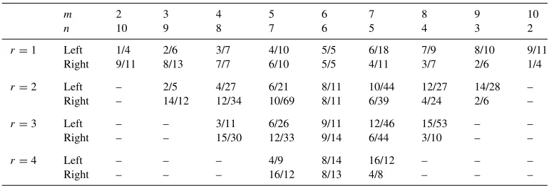
Table 1
Number of optimization variables and average iterations for the optimization algorithm solving (WLRA) by left and right kernel representations
m 2 3 4 5 6 7 8 9 10
n 10 9 8 7 6 5 4 3 2
r=1 Left 1/4 2/6 3/7 4/10 5/5 6/18 7/9 8/10 9/11
Right 9/11 8/13 7/7 6/10 5/5 4/11 3/7 2/6 1/4
r=2 Left – 2/5 4/27 6/21 8/11 10/44 12/27 14/28 – Right – 14/12 12/34 10/69 8/11 6/39 4/24 2/6 –
r=3 Left – – 3/11 6/26 9/11 12/46 15/53 – – Right – – 15/30 12/33 9/14 6/44 3/10 – –
r=4 Left – – – 4/9 8/14 16/12 – – – Right – – – 16/12 8/13 4/8 – – –
w=rand(m∗n,2∗m∗n);w=w∗w;
dt=reshape(sqrtm(w)\randn(m∗n,1),m,n);
dt=dt/norm(dt,fro); %normalization
d=d0+0.001∗dt;
The matrix dimensionmis varied from 2 to 10 andn:=12−m. The desired rankris varied from 1 to 4. For each combination ofmandr,N =50 independently generated data matrices are generated and for each one of them the problems (WLRA) with left and right input/output representations are solved.
We use the Levenberg–Marquardt optimization algorithm from the Optimization toolbox of MATLAB (lsqnonlin) with cost function evaluations only. In both cases (left and right in-put/output representation), the algorithm is run from equivalent initial approximations obtained using the singular value decompositions (unweighted low-rank approximation) and the stopping criteria are set to the same tolerances. In this particular experiment, in all runs the same solution was found by using the two representations. As expected the average number of iterations, how-ever, depends on the number of optimization parameters (elements ofXandXr): the fewer the
optimization variables, the fewer the average number of iterations for convergence. Numerical results are shown in Table 1 in the format “# of optimization variables/# of iterations”.
5. Special cases of column and row-weighting
Up to now we have considered the WLRA problem with a full weight matrixW. Of interest, however, are the two special cases of element-wise weighting, i.e.,W diagonal, column-wise weighting, i.e.,Wblock diagonal with blocks of dimensionm×m, and row-wise weighting, i.e., TW T block diagonal with blocks of dimensionn×n, whereT is themn×mnpermutation matrix, such that vec(D)=Tvec(D). The special structure ofW can be exploited for efficient cost function and first derivative evaluation.
ˆ
dIM:=(I⊗P )((I⊗P )W (I⊗P ))−1(I⊗P )W d
⇔ ˆdIM,i =P (PWiP )−1PWidi,
wherediis theith column ofDanddˆiis theith column ofD. Similar decoupling into independent
terms occurs for the left kernel representation: ˆ
dKER=
Imn−W−1(I⊗R)
(I⊗R)W (I⊗R)
−1
(I⊗R)
d
⇔ ˆdKER,i=
Im−Wi−1R(RWiR)−
1
R di.
In the case of right image and right kernel representations the computational savings are achieved as follows. For the right image representation
ˆ
drIM:=(L⊗Im)
(L⊗Im)W (L⊗Im)
−1
(L⊗Im)W d, (*)
denoting theith column ofLbyli, we have
(L⊗Im)W (L⊗Im)=
l1⊗Im · · · ln⊗Im
× ⎡ ⎢ ⎣
W1
. .. Wn
⎤ ⎥ ⎦
⎡ ⎢ ⎣
l1 ⊗Im
.. . ln ⊗Im
⎤ ⎥ ⎦="n
i=1
lili⊗Wi.
Let
p:= # n
"
i=1
lili ⊗Wi
$−1
l1⊗W1 · · · ln⊗Wn
d (**)
andP :=p1 · · · pr
, wherep=:p1 · · · pr
andpi ∈Rm. Note thatp=vec(P ).
Finally, ˆ
drIM=(L⊗Im)p⇒DrIM=P L.
Computingpusing (**) and settingDrIM=P Lis a more efficient alternative to the direct
computation ofdˆrIMusing (*).
6. Conclusions
We have presented four representations of the rank constraint that turn the abstract weighted low-rank problem formulation in concrete parameter optimization problems. The optimization problem was solved analytically for the approximating matrixD, which resulted in an equivalent optimization problem over the parameters of the rank representation only. We showed a unique parameterization that avoids the quadratic constraint and further transforms the optimization problem into a classical nonlinear least squares problem. Finally we showed how the cost function can be computed efficiently in two special cases: row-wise and column-wise weighting.
Acknowledgments
grants; Flemish Government: FWO: PhD/postdoc grants, projects, G.0360.05 (EEG signal pro-cessing), G.0321.06 (numerical tensor techniques), research communities (ICCoS, ANMMM); IWT: PhD Grants; Belgian Federal Science Policy Office IUAP P5/22 (‘Dynamical Systems and Control: Computation, Identification and Modelling’); EU: BIOPATTERN, ETUMOUR; HEALTHagents.
References
[1] B. De Moor, Structured total least squares andL2approximation problems, Linear Algebra Appl. 188–189 (1993)
163–207.
[2] G. Eckart, G. Young, The approximation of one matrix by another of lower rank, Psychometrika 1 (1936) 211–218. [3] K. Gabriel, S. Zamir, Lower rank approximation of matrices by least squares with any choice of weights,
Techno-metrics 21 (1979) 489–498.
[4] J. Manton, R. Mahony, Y. Hua, The geometry of weighted low-rank approximations, IEEE Trans. Signal Process. 51 (2) (2003) 500–514.
[5] I. Markovsky, M.-L. Rastello, A. Premoli, A. Kukush, S. Van Huffel, The element-wise weighted total least squares problem, Comput. Statist. Data Anal. 50 (1) (2005) 181–209.
[6] I. Markovsky, J.C. Willems, S. Van Huffel, B. De Moor, Exact and Approximate Modeling of Linear Systems: A Behavioral Approach, Monographs on Mathematical Modeling and Computation, vol. 11, SIAM, 2006.
[7] A. Premoli, M.-L. Rastello, The parametric quadratic form method for solving TLS problems with elementwise weighting, in: S. Van Huffel, P. Lemmerling (Eds.), Total Least Squares and Errors-in-Variables Modeling: Analysis, Algorithms and Applications, Kluwer, 2002, pp. 67–76.
[8] C. Paige, Z. Strakos, Core problems in linear algebraic systems, SIAM J. Matrix Anal. Appl. 27 (2005) 861–875. [9] M. Schuermans, I. Markovsky, P. Wentzell, S. Van Huffel, On the equivalence between total least squares and
maximum likelihood PCA, Anal. Chim. Acta 544 (2005) 254–267.
[10] C. Van Loan, N. Pitsianis, Approximation with Kronecker products, in: M. Moonen, G. Golub (Eds.), Linear Algebra for Large Scale and Real Time Applications, Kluwer Publications, 1993, pp. 293–314.
[11] S. Van Huffel, J. Vandewalle, Analysis and solution of the nongeneric total least squares problem, SIAM J. Matrix Anal. Appl. 9 (1988) 360–372.
[12] S. Van Huffel, J. Vandewalle, The Total Least Squares Problem: Computational Aspects and Analysis, SIAM, Philadelphia, 1991.