Impact of demand-side management on substations

(1)

(2)

University of Southern Queensland

Faculty of Engineering and Surveying

IMPACT OF DEMAND-SIDE

MANAGEMENT ON SUBSTATIONS

A dissertation submitted by

David Thomas Chalmer GRAY

in fulfilment of the requirements of

Course ENG4111/ENG4112 Project

towards the degree of

(3)

Table of Content

Abstract...1

Certification...3

Acknowledgments ...4

Nomenclature ...5

Glossary ...6

1. Background ...9

1.1 Introduction... 9

1.2 What is Demand-Side Management... 10

1.3 Project Justification... 11

1.4 Project Aims... 11

1.5 Understanding of Demand-Side Management Impact ... 11

1.6 Possible Impacts of Change ... 12

2. Demand-Side Management Systems ...14

2.1 Control Theory... 14

2.1.1 Introduction to Load Control Theory ... 14

2.1.2 Type of Load Control Used ... 15

2.1.3 ABB Master Station LCM-500 (Load Control Master 500) ... 15

2.2 Theory of Tariff Arrangements ... 16

2.2.1 Introduction of Tariff Arrangements ... 16

2.2.2 The Application of Tariff Switching ... 16

2.3 Other Forms of Load Control/ Demand-Side Management ... 17

2.3.1 Other forms of Load Control... 17

2.3.2 Power Factor Correction ... 17

2.3.3 Voltage Reduction ... 18

2.3.4 Frequency Reduction... 19

2.3.5 Private Generation ... 19

2.4 Relevant Standards... 20

2.5 Relevant Codes ... 20

2.6 Technical References ... 21

3. Project Methodology...23

3.1 Methodology Introduction ... 23

3.2 Preliminary Tasks ... 23

3.2.1 Technical Research ... 23

3.2.2 Choice of Substations ... 23

(4)

3.2.4 Determination of Tariff Switching Times ... 24

3.3 Report... 24

3.3.1 Data... 24

3.3.2 Analysis Dates ... 25

3.3.3 Analysis ... 25

3.3.4 Conclusions ... 25

4. Data Analysis and Results ...27

4.2 Nemmco Load Profiles ... 28

4.2.1 Discussion on Figure 6 and Figure 7... 28

4.3 Substation Number 1... 29

4.3.1 Substation Number 1 Configuration... 29

4.3.2 Load growth for Substation Number 1 ... 29

4.3.3 Substation Number 1 Transformer Load Summary ... 30

4.3.4 Substation 1 Transformer Summary... 30

4.3.5 Substation Number 1 Example of Domestic Feeder ... 31

4.3.6 Substation 1 Domestic Feeder Summary... 31

4.3.7 Substation Number 1 Example of Industrial Feeder... 32

4.3.8 Substation 1 Industrial Feeder Summary ... 32

4.4 Substation Number 2 Data ... 33

4.4.2 Load growth for Substation Number 2 ... 33

(5)

4.9.5 Substation Number 7 Example of Domestic Feeder ... 55

4.9.9 Substation Number 7 Example of Capacitor Bank Operation... 57

4.9.10 Substation 7 Capacitor Bank Summary ... 57

4.10 Substation Number 8 Data... 58

4.10.1 Substation Number 8 Configuration ... 58

4.10.4 Substation Number 8 Example of Feeder... 60

4.10.5 Substation 8 Feeder Summary ... 60

(6)

4.11.1 Substation Number 9 Configuration ... 61

4.11.6 Substation 9 Domestic Feeder Summary ... 63

4.11.7 Substation Number 9 Example of Domestic / Industrial Feeder... 64

4.11.8 Substation 9 Industrial Feeder Summary... 64

4.12 Discussion of Results... 65

4.12.1 6pm Load peaks ... 65

4.12.2 Low feeder power factor ... 66

4.12.3 Air-conditioning... 67

4.12.4 Improved demand-side management options... 67

4.12.5 Capacitor Bank effectiveness ... 67

5. Discussion ...69

5.2 Air-Conditioning Load... 69

5.2.1 Introduction... 69

5.2.2 Tariff Control ... 70

5.2.3 Thermostat Adjustment... 70

5.2.4 Load Cycling ... 71

5.2.5 Congestion Pricing... 71

5.2.6 Conclusion... 72

5.3 Under Frequency Load Shedding... 73

5.4 Rotational Load Shedding... 74

5.5 Voluntary Load Shedding ... 75

5.6 Retail Pricing... 75

5.7 Energy Conservation... 76

5.8 Energy Storage... 76

5.9 Temperature Effects on Plant... 77

5.10 Issues and Assumptions... 77

6. Conclusions and Recommendations ...79

6.1 Project Objectives ... 79

6.1.1 Review of Demand-Side Management Options ... 79

6.1.2 Assessment of current documentation ... 80

6.1.3 Gathering and Analysis of data... 80

(7)

6.2.4 Customer Liaison ... 81

6.3 Conclusion ... 81

Reference List...82

List of Tables

Table 1- List of Substations for Analysis ...23

Table 2 - Summary of Substation Number 1 Data ...29

Table 7- Summary of Substation Number 6 Data ...49

Table 11 - Table of signal sent for Tariff 33 switching between 6pm and 10pm...65

Table 12 - Table of frequency and timings for Under Frequency Load Shedding...73

Table 13 - Table of Ergon Energy Corporation Tariff Arrangements...88

List of Figures

Figure 1: Overview of General Load Control Configuration ...15

Figure 2- Example of the switching patterns for receivers for various tariffs...16

Figure 3 – Reactive Power triangle ...17

Figure 4 - Capacitive Power triangle...17

Figure 5 - Power triangle after the affects of a Capacitor Bank are included...18

Figure 6 – Graph of total DNSP load for 15th_{July 2003...28}

Figure 7 - Graph of total DNSP load for 9th_{December 2003...28}

Figure 8 - Graph of Load Growth for 5 years for Substation 1 ...29

Figure 9 - Graph of the Total Winter Load on Substation 1...30

Figure 10 - Graph of the Total Summer Load on Substation 1 ...30

Figure 11 - Graph of the Winter Load on Substation 1 Feeder 2 ...31

Figure 12 - Graph of the Summer Load on Substation 1 Feeder 2...31

Figure 15 - Graph of Substation 2 Load Growth for the past 9 years...33

(8)

Figure 43- Graph of Load Growth for 13 years for Substation 6 ...49

(9)

Figure 57 - Graph of the Winter Load on Substation 7 Capacitor Bank ...57

Figure 58 - Graph of the Summer Load on Substation 7 Capacitor Bank...57

Figure 68 - Graph of Residential air-conditioning load curve...69

Figure 69 - Graph of Average Temperature Maximum and Minimum...90

Figure 70 – Graph of Typical Retail Electricity Prices for 24 hour ...92

Figure 71 – Close up graph of Typical Electricity Prices...92

Appendix List

Appendix 1 - Project Specification...84

Appendix 2 - Summary of the Queensland Tariff Arrangement ...86

Appendix 3 – Graph of Average Maximum and Minimum Temperature...89

Appendix 4 - Example of a Daily Electricity Price Schedule ...91

(10)

Abstract

With the significant increase in the consumption of electricity over the past few years, it has been hard for electricity entities to keep up with the sudden increases in demand. The

replacement and upgrade of substation transformers and associated equipment is very

expensive and time consuming to obtain and install. Also the wanton use of electricity

without understanding the consequences and its impact on the environment is negligent

on the part of the individual.

For the purpose of this project Demand-Side Management is any action taken to reduce the

consumption of electricity supply to a customers premises, to assist an Electricity Entity

in the stability of the electricity network. This leads to the principle that Demand-Side

Management can be used to defer capital expenditure by attempting to average a feeder

or substation load over a longer period and reduce the amount of peaks and troughs.

As will be seen later in the report, air-conditioning load is one of the fastest growing

domestic loads, with significant increases over the past 2 to 3 years. As a result the

electricity networks are being overloaded due to the unexpected increase in electricity

demand.

There are many different methods of demand-side management mentioned in this

report, most of these can be used to manage air-conditioner load, however the methods

would not be acceptable to customers.

After looking at various forms of demand-side management I believe that congestion

pricing is the method that is most suitable and fair for managing customers

air-conditioning load. Congestion pricing operates similar to tariff control, however the

difference is that electricity prices are increased during high demand periods.

(11)

University of Southern Queensland

Faculty of Engineering and Surveying

ENG4111 & ENG4112 Research Project

Limitations of Use

The Council of the University of Southern Queensland, its Faculty of Engineering and

Surveying, and the staff of the University of Southern Queensland, do not accept any

responsibility for the truth, accuracy or completeness of material contained within or

associated with this dissertation.

Persons using all or any part of this material do so at their own risk, and not at the risk

of the Council of the University of Southern Queensland, its Faculty of Engineering and

Surveying or the staff of the University of Southern Queensland.

This dissertation reports an educational exercise and has no purpose or validity beyond

this exercise. The sole purpose of the course pair entitled "Research Project" is to

contribute to the overall education within the student’s chosen degree program. This

document, the associated hardware, software, drawings, and other material set out in the

associated appendices should not be used for any other purpose: if they are so used, it is

entirely at the risk of the user.

Prof G Baker

Dean

(12)

Certification

I certify that the ideas, designs and experimental work, results, analyses and conclusions set out in this dissertation are entirely my own effort, except where otherwise indicated and acknowledged.

I further certify that the work is original and has not been previously submitted for assessment in any other course or institution, except where specifically stated.

David Thomas Chalmer GRAY

Student Number: 0018165616

__________________________

(Signature)

__________________________

(13)

Acknowledgments

I would like to acknowledge and thank:

Mr. Ron Sharma – Faculty of Engineering and Surveying, University of Southern Queensland

Mr. Ken Lewis – Network Operations Analysis Manager, Ergon Energy Corporation

Mr. Malcolm Adkins – Network Forecast Officer, Ergon Energy Corporation

Mr. Wayne Ivers – Metering Support Technical Officer, Ergon Energy Corporation

My wife, Tina and children Jordyn, Alexandra and Hamish

DAVID GRAY

University of Southern Queensland

(14)

Nomenclature

Term Description Units

A Amperes A

f Frequency Hz

GVA Giga Volt Amperes GVA

I2R Reactive Power Losses

kV kilo Volts kV

kVA kilo Volt Amperes kVA

MVA Mega Volt Amperes MVA

MWh Mega Watt hours MWh

P Real Power W

pf Power Factor

-p Phi

-Q Reactive Power VAr

S Active Power VA

q Theta º or

radians

V Volts V

VA Volt Amperes VA

VAr Volt Amperes Reactive VAr

W Watts W

XL Reactive Impedance W

(15)

Glossary

¨ ABB – Asea Brown Boveri Company

¨ Bund Wall – Is a raised wall around the outside of a transformer to prevent oil spills

¨ Contestable Customers - Contestable customers are generally customers whose electricity consumption exceeds 200MWh/ year

¨ Domestic – Refers to a customer who consumption of electricity is primarily for personal use

¨ DNSP – Is a distribution network service provider like Ergon Energy Corporation or Energex Corporation who manage the supply of electricity to customers

¨ Electricity Act 1994 – An act of parliament that contains the laws that govern the supply and use of electricity around Queensland

¨ Electricity Retailer – Is the retail side of an electricity business and is the primary interface for customers

¨ Ergon Energy Corporation – Is the distribution company of Ergon Energy controls and maintains the poles, wires and assets for regional Queensland

¨ Ergon Energy Pty Ltd – Is the retail company of Ergon Energy who manages the customer interface and sale of electricity around Australia

¨ Franchise Customers – Also referred to as a Market Customer, is a customer who is entitled to purchase power from any registered electricity retailer

¨ Industrial – Refers to a customer who consumes electricity to carry out a business, it must be noted that not all businesses will exhibit an industrial load consumption

¨ Load Control Unit – Is a system used to turn electricity on and off or to change an electricity meter between high and low tariff

¨ N-1 – This means that the loss of a single piece of plant will not cause an outage to occur

(16)

¨ NEMMCO – Is the National Electricity Market Management Company and oversee the stability of the electricity network around Australia by managing the interface between the Electricity Generators, TNSP and DNSP’s

¨ Tariff – Is a method of offering customers lower priced electricity to consume power off peak, or at a time that will offer less impact on the electricity network

(17)

C

HAPTER

1

(18)

1.

Background

1.1

Introduction

With the ever-increasing use of electricity across the country and around the world, it is hard for electricity entities like Ergon Energy Corporation to keep up with sudden increases in demand. The replacement and upgrade of substation transformers and associated equipment is very expensive and time consuming to obtain and install. Also the wanton use of electricity without understanding the consequences and its impact on the environment is negligent on the part of the individual. It is therefore incumbent on electricity entities to manage the load and attempt to mitigate the impact of the load on the entity assets.

All electricity corporations in the state of Queensland are required to offer franchise customers a reduction in cost of electricity supply by varying the times that supply is available. Contestable customers are not required to be offered tariff controlled electricity at reduced prices as they are offered electricity at a rate different to non-contestable customers. The most common type of electricity load that customers choose to vary is for the heating of hotwater for domestic installations and fixed plant, such as permanently connected dishwashers, dryers and to a larger extent air-conditioners. Hotwater load is usually supplied by electricity at non-peak demand times, this is done by utilising various tariffs. By doing this, the overall impact on the electrical system can be reduced, by attempting to reduce the peak demand in the supply of electricity.

(19)

1.2

What is Demand-Side Management

‘What is Demand Side Management?’ this question can raise more issues than one might originally think. Demand Side Management can be and is viewed differently by each organisation and even people within the organisation.

“Demand Side Management refers to the actions taken on the customer’s side of the meter to change the amount or timing of energy consumption.” (US Department of Energy, 2004)

However, discussions with operational staff in Ergon Energy Corporation suggest that Demand Side Management is where a customer is guided to make appropriate choices to suit the Electricity Entities capabilities. This type of philosophy will assist the DNSP is managing the electricity network and is not just a sales tool for an Electricity Retailer.

So as can be seen the question of ‘What is Demand Side Management?’ alone can create a large debate, however subtle the differences are. For the purpose of this document Demand Side Management will be referred to as:

Actions taken to reduce the consumption of electricity supply to the customer premises, to assist a Distribution Network Service Provider in the stability of the electrical network.

Demand Side Management is achieved by two main methods:

1. Load Reduction – Load reduction refers to the reduction of electricity by means of the installation of energy saving technologies and other forms of energy reduction methodologies, for example, load reduction agreements with customers.

2. Load Levelling – Load levelling refers to smoothing out the peaks and dips in energy supply. Some form of Load Control generally performs load levelling and this is the area that is of particular interest in this report.

(20)

1.3

Project Justification

A new substation with a typical 2 by 10MVA transformer capacity costs approximately $6Million to construct. This would include the cost of purchase and installation of the transformer and other ancillary items like protection, circuit breakers, busbar, civil works, buildings and feeder installation. This cost is often compounded when upgrading an older substation.

For example a 2 x 16MVA substation with 16MVA of load needs to be upgraded to a 2 x 25MVA substation, with this change there is a requirement to upgrade other pieces of plant within the substation. Some of these included new Bund walls for oil containment, new transformer circuit breakers, protection upgrades including new protection relays, current and voltage transformers and quite often re-configuring the substation layout. This change would typically cost around $2.3Million and relies on the major portion of the current substation equipment being able to be reused.

As can be seen the cost of upgrading a substation is substantial, so if an upgrade project can be delayed then the cost savings can be significant. For example a $2 million project delayed by four years could have an annual saving of approximately $200,000 per annum. This allows for the saving to be spent on assets that can have a greater impact on improving the electricity network reliability.

1.4

Project Aims

The aim of the project is to determine what is the actual impact of Demand-Side Management in substations. This will be achieved by analysing the load profiles of various substations and determining what has been the impact of the tariff switching on the substation. Currently Queensland’s predominate form of Demand-Side Management for load control is through tariff control (tariff control will be explained further in the next chapter - Chapter 2).

Once the impact of tariff load control has been determined, further analysis will look at whether or not other forms of Demand-Side Management will be beneficial.

1.5

Understanding of Demand-Side Management Impact

(21)

Part of the purpose of this report is an attempt to raise the understanding of different methods of dealing with Demand-Side Management.

1.6

Possible Impacts of Change

There are a number of topics that may be impacted by this project:

· A change may be needed to the current tariff arrangements, an example maybe that Tariff 31 may mean a change such that the customer still gets 8 hours but instead of being between 10pm and 7 am, it may need to be between 8pm and 8am (This is an illustrative example only).

· A change of view may be required to what Demand Side Management actually is, instead of just tariff control, it might extend to hedging offers where a customer of a certain size is given 24 hours notice to reduce load by 50%.

(22)

C

HAPTER

2

D

EMAND

-S

IDE

(23)

2.

Demand-Side Management Systems

2.1

Control Theory

2.1.1

Introduction to Load Control Theory

Load Control can be carried out at two (2) separate locations:

1. Manually from a central location to de-centralised Load Control Units.

In the case of a Manual Control a control signal is sent to the required de-centralised Load Control Unit which then instigates for an open or close signal to be sent to the remote receivers, as can be seen in the diagram 1 below. This is generally only done when there is a problem on the electrical supply system or there has been a request from the Electricity Supply Retailer to shed loads for Electricity market manipulation; or

2. Automatically from the pre-programmed de-centralised Load Control Unit.

(24)

[image:24.595.129.489.67.357.2]

Figure 1: Overview of General Load Control Configuration

2.1.2

Type of Load Control Used

The Central Region of Ergon Energy Corporation has two main types of Load Control being used these are ABB and Enermet. The ABB master station system is briefly described below in 2.1.3.

2.1.3

ABB Master Station LCM-500 (Load Control Master 500)

The LCM-500 master station is a fully automatic control and monitoring system for the management of load. It operates using audio frequency ripple control technology where information is passed over the electricity entity wires. The system has the following functions:

¨ Man-machine interface

¨ Message processing and station monitoring

¨ Analysis of network load and other analogue values

¨ Load management functions

Control Centre

De-Centralised

Area 1

Area 2

(25)

2.2

Theory of Tariff Arrangements

2.2.1

Introduction of Tariff Arrangements

All electricity supply is bound by various legal and business requirements, part of those requirements are for customers to be offered supply at a certain cost for being on a specified tariff. These tariffs also have limitations placed on them under the Electricity Act 1994 and by the Electricity Retailer. A summary of the tariffs for the state of Queensland is listed in Appendix 2.

Some of the limitation and constraints placed on the Electricity Supplier are the maintenance of supply to a customer for a specified period for any 24-hour period, several examples are included below:

Tariff 31 customer must have 8-hour availability of supply between 10pm and 7am or an 8-hour block of supply as determine by the Electricity Supplier.

Tariff 65 customers are Irrigation – Time of Use Customers that are charged at 12 hours “High” rate and 12 hours at “Low” rate. That is to say that when the tariff is on the “High rate” the customer pays more for their electricity than when they are the “Low rate”.

2.2.2

The Application of Tariff Switching

Central Region Ripple Telegrams consist of a 50 bit coded message injected onto the network by a ripple control injection plant. The 50 on/off pulses (bits) are interpreted by the receiver, then any commands associated with the received message are activated.

The 50 bits are divided into groups, whereby each group of bits defines a characteristic of the message being transmitted. An example of the from switching patterns is shown below:

Tarrif Time 03:00 06:00 07:00 08:00 09:00 10:00 11:00 12:00 13:00 14:00 15:00 16:00 17:00 18:00 19:00 20:00 21:00 22:00 23:00 24:00

T31

T33

Low Rate Low Rate

T22 & T62 High Rate

T65 (1) Low Rate Low Rate

High Rate

Low Rate Low Rate

T37 High Rate

Snchronisation Pulse, sets reciever clock to 3am

(26)

2.3

Other Forms of Load Control/ Demand-Side Management

2.3.1

Other forms of Load Control

Until now only tariff based load control has been covered, this is because it is the predominate form of load management currently being used. However, there are other forms of load management, some of which are not so widely used. Below are several of the more common methods that are utilised.

2.3.2

Power Factor Correction

Power Factor correction is generally carried out substation level, but what is power factor correction. Power factor correction effectively reduces the total flow through the power network by local injection or absorption of imaginary power to match the corresponding customer production levels. This reduces overall power system energy I2_{R losses, and allows improved}

asset utilisation by freeing up network plant capacity for real power transmission. Power factor correction is based on the principle of reducing the reactive power by counteracting the reactive power with a capacitive power correction (Grainger & Stevenson 1994).

1 1 1

P

jQ

S

=

+

Figure 3 – Reactive Power triangle

2 2 2

P

jQ

S

=

+

Figure 4 - Capacitive Power triangle

S1 is a representation of load based on a substation as Q1 the reactive power increases.

q1 = atan (Q1/P1 ) increases the power factor pf1 = cos q1 decreases. So if pf = 1 then q = 0º and

if pf = 0.9 then _q = 25.8º. As can be seen as the power factor decreases the angle _q increases

and as _q increases the reactive power increases and therefore the overall power increases. Capacitive power works in the opposite direction to reactive power and counteracts the effects of the reactive power. So when the effects of the Capacitor Bank are included in the system the impact of the reactive power on the electrical system in general and in particular at a substation is reduced.

Q1

S1

P1

q1

P2

S2 Q2

(27)

Figure 5 - Power triangle after the affects of a Capacitor Bank are included

The overall power can be broken up such that the reactive power Q3 is now Q1 + Q2, however

because Q2 is in the capacitive it is in the negative direction. P3 = P1 + P2 and

S

3

=

P

32

+

Q

32

.

Therefore by adding capacitor banks to the electrical system the overall power consumed can be reduced as well as improving the power factor.

2.3.3

Voltage

Reduction

This form of load management can be used at the lower high voltages, i.e.11 and 22kV. Voltage reduction works on the basic principle of V = I*Z and relies on the fact that the majority of load at the distribution level is a constant impedance. Therefore by reducing the voltage, the current will be reduced proportionately.

For example: Let I = 100A, V = 22,000 V and Z be a constant impedance.

\22,000 = 100 x Z

\Z = 220 _W

By maintaining the constant impedance and reducing the voltage to 20kV, the current can be reduced to 90.91 A. As can be seen the current flow is reduced by approximately 10% or the same proportion as the voltage is reduced. This form of control is particularly useful for relieving overload situations on 11 and 22 kV feeders without turning customers supply off. The down side is that when there is a constant power load on the system, by reducing the voltage the current can increase.

q1

q2

(28)

2.3.4

Frequency

Reduction

Frequency reduction is used primarily for motor starting and will have no impact on anything but the reactive aspect of a load. This can be proven by the following formula (Grainger & Stevenson 1994):

Example 1:

Let assume that the inductance (L) is 100mH and a frequency (f) of 50Hz.

W

=

2

fL

2

*

50

*

100

x

10

-3

31

.

4

X

_L

p

Example 2:

Let assume that the inductance (L) is 100mH does not change however the frequency (f) changes to 45Hz.

W

=

2

fL

2

*

45

*

100

x

10

-3

28

.

3

X

_L

p

As can be seen by reducing the frequency the reactive impedance XL is reduced.

2.3.5

Private

Generation

One of the most fashionable forms of system grid load reduction at the moment is private generation. Private generation can take several forms from Photovoltaic Cells on a customer’s roof to a large gas fired generator. Ergon Energy Corporation has stepped into the market place with the world’s first “green electricity” powerplant. Ergon Energy Corporation and SunCoast Gold Macadamias have built and are operating a 1.5MW generator near Gympie Queensland that is fuelled by macadamia nut shells.

(29)

2.4

Relevant Standards

There are essentially three separate standards, that relate to tariffs, these are:

· AS 1284.6 – 1992 Electricity metering, Part 6: Ripple control receivers for tariff and load control.

· AS 1284.10.1 – 1996 Electricity metering, Part 10.1: Data exchange for meter reading and load control – Direct local data exchange via hand-held unit (HHU) – IEC Standard interface.

· AS 1852(691) – 1975 International Electrotechnical Vocabulary, Chapter 691: Tariffs for electricity.

2.5

Relevant Codes

There are two different sources that make reference to code one at a state level, the other at a National level. At a Queensland state level we have:

· Section 62 and 90 of the Electricity Act 1994 allow for the Minister to decide on the prices, or the methodology to fix the prices, that a retail entity may charge. This allows for the tariff arrangements to be put in place and varied by Government intervention. In 2003 the retail electricity price where changed, via Queensland Government Gazette, June 2003, No. 47.

(30)

2.6

Technical References

The majority of the technical reference papers and reports in circulation have been commissioned by a Distribution Network Service Provider, Electricity Retailers or other Government agencies to deal with methods of impacting on the retail price of electricity.

However, Integral Energy commissioned a report titled “DM Programs for Integral Energy” prepared by Charles River Associates (Asia Pacific) Pty Ltd in August 2003. There is a significant amount of information in this report that was prepared for Integral Energy that relates to the various Demand Management Strategies and how these strategies can impact on the Electrical Supply Network.

(31)

C

HAPTER

3

(32)

3.

Project Methodology

3.1

Methodology Introduction

This section covers the overall methodology used for developing this report. It will cover the preliminary tasks, gathering of metering data, the layout of the report and the reasoning behind the choices made.

3.2

Preliminary Tasks

3.2.1

Technical

Research

The initial information gathering exercise to determine how demand-side management is being handled in Ergon Energy Corporation. This information came primarily from the Metering department, Planning department and various technical manuals associated with the specific technology being used for tariff management.

3.2.2

Choice of Substations

The number of substations that have been chosen for this project has been limited to nine (9) all located in Rockhampton and surrounding area (List included in below Table 1). This was done to assist in the data gathering exercise and to allow ready access to the substations for further detailed assessment. The data presented in the Results Chapter does not have the respective substation name attached. This has been done for confidentiality purposes.

Substation

Yeppoon Lakes Creek

Rockhampton Glenmore Parkhurst

Pandoin Frenchville

Rockhampton South Malchi

(33)

3.2.3

Gathering and Analysis of Substation Data

The gathering and analysis of the metering data for each of the substations that have been chosen was time consuming and meant utilising Microsoft Access to manipulate the data to produce information that was useful for further analysis purposes.

The tariff 31 and tariff 33 switching times and power factor for each of the feeders was also obtained and superimposed onto the feeders and substation data to give a visual representation of how effective current methods of demand-side management methods are.

3.2.4

Determination of Tariff Switching Times

The next step after gathering the substation metering data was to try to match the tariff switching times against the load profiles obtained. This will be done utilising the master controller signalling times to determine when a particular tariff is turned on and off. This will then give a visual representation of the impact of the load control methodology on substations and should show how effective the current load control practices are in demand-side management.

3.3

Report

The final report should cover off the following issues:

3.3.1

Data

The data has been presented in an easy to read format, representing a summer and a winter load profile for each substation for:

¨ The substation overall;

¨ An Industrial feeder; and

¨ A domestic feeder.

(34)

3.3.2

Analysis

Dates

The dates to be analysed are the 15th_{July 2003 and 9}th_{December 2003, these dates where}

chosen to account for the extremes of temperature for winter and summer in Appendix 3 shows the Bureau of Meteorology report for the respective days. A Wednesday was chosen in an attempt to clearly show the comparison between industrial and domestic feeder loads.

3.3.3

Analysis

All assumptions made during the analysis of the data are detailed and explained in Chapter 5 Discussion.

3.3.4

Conclusions

(35)

C

HAPTER

4

D

ATA

A

NALYSIS

AND

(36)

4.

Data Analysis and Results

4.1

Introduction

The data presented in this section is a summary of the data that was extracted from each of the substations metering data. The data has been presented in graph format with an analytical description afterward. If all graphs of each feeder for the nine substations where included then the data would be excessively repetitive and not add any value to the analysis. So therefore graphs of only two feeders and the total substation load have been included, and at the end of the analysis a feeder that has an “ideal” load profile will be included for comparison.

(37)

4.2

Nemmco Load Profiles

Figure 6 – Graph of total DNSP load for 15th July 2003

Figure 7 - Graph of total DNSP load for 9th_{December 2003}

4.2.1

Discussion on Figure 6 and Figure 7

The data shown in Figure 6 and Figure 7 is data gathered from NEMMCO public records. The graphs are summation of Ergon Energy Corporation and Energex Corporation loads for the 15th July and 9th_{December 2003.}

As can be seen the summer load is approximately 130% of the winter load. Whilst some of this is due to load growth data presented after each substation configuration shows how much the load in each substation has risen in the past few years. Most of this summer load increase is due to air-conditioning.

Total Queensland Load - 15/07/03

0 50 100 150 200 250 300

Tim e (hrs)

GV

A

Qld Total T33 T31

T otal Qu een sland L oad - 09/12/03

0 50 100 150 200 250 300 350 400

Tim e (hrs )

GVA

(38)

4.3

Substation Number 1

4.3.1

Substation Number 1 Configuration

Substation 1 has the following configuration:

Transformers 2 by 25 MVA 66/11kV 2 by 10MVA 66/22kV

Capacitor Bank 2 by 4 MVAr @ 11kV

Number of Feeders 6 @ 11kV 2 @ 22kV

Ripple Control Nil

Peak Load 20.41 MVA

Number of Customers 10,316

Table 2 - Summary of Substation Number 1 Data

4.3.2

Load growth for Substation Number 1

Figure 8 - Graph of Load Growth for 5 years for Substation 1

0 5 10 15 20 25 30 Jul-0 0 Sep-0 0 Dec-0 0 Mar-01Jun-0 1 Sep-0 1 Dec-0 1 Mar-0 2 Jun-0 2 Sep-0 2 Dec-0 2 Mar-03Jun-0 3 Sep-0 3 Dec-0 3 Mar-0 4 Jun-0 4 MW 0% 10% 20% 30% 40% 50% 60% 70% 80% 90% 100% Monthly Max Demand (MW) - Substation 1 - Sub Total (Transformer 11 kV)

LF

(39)

4.3.3

Substation Number 1 Transformer Load Summary

Figure 9 - Graph of the Total Winter Load on Substation 1

Figure 10 - Graph of the Total Summer Load on Substation 1

4.3.4

Substation 1 Transformer Summary

Load:

The first of the two peaks in the winter load (Figure 9) is around dinnertime, also a review of the tariff 33 switching times indicates that Channels 1, 4 and 6 being turned on corresponds to this peak as well. The interesting thing about the summer load (Figure 10) is the manner in which the load ramps up from early morning. This tends to indicate air-conditioning load progressively ramping up as the ambient temperature gets hotter throughout the day.

Power Factor:

In this case the power factor for both Figure 9 and Figure 10 is stable. T31

T33

Sub 1 - Transformer 15/07/03

0 2 4 6 8 10 12 14 16 18 0: 00 1: 30 3: 00 4: 30 6: 00 7: 30 9: 00 10: 30 12: 00 13: 30 15: 00 16: 30 18: 00 19: 30 21: 00 22: 30 Time (hrs) MVA 0.88 0.9 0.92 0.94 0.96 0.98 1 1.02

TFR Load T33 T31 pf

Sub 1 - Transformer 09/12/03

0 2 4 6 8 10 12 14 16 18 0: 00 1: 30 3: 00 4: 30 6: 00 7: 30 9: 00 10: 30 12: 00 13: 30 15: 00 16: 30 18: 00 19: 30 21: 00 22: 30 Time (hrs) MVA 0.88 0.9 0.92 0.94 0.96 0.98 1 1.02

(40)

4.3.5

Substation Number 1 Example of Domestic Feeder

Figure 11 - Graph of the Winter Load on Substation 1 Feeder 2

Figure 12 - Graph of the Summer Load on Substation 1 Feeder 2

4.3.6

Substation 1 Domestic Feeder Summary

Load:

The load varies greatly during the winter period (Figure 11) however, the summer load (Figure 12) is very good representation of a domestic feeder with relatively no load between business hours and high loads after hours. Of concern in the summer load is the nature of the afternoon peaks, these indicate that there maybe high air-conditioner usage at dinnertime, then a second peak at approximately 2300 hrs where the hotwater tariff switches on.

Power Factor:

The interesting thing about the power factor in summer (Figure 12) in

Fdr 2 15/07/03

0 0.5 1 1.5 2 2.5 3 0: 00 1: 30 3: 00 4: 30 6: 00 7: 30 9: 00 10: 30 12: 00 13: 30 15: 00 16: 30 18: 00 19: 30 21: 00 22: 30 Time (hrs) MVA 0.86 0.88 0.9 0.92 0.94 0.96 0.98 1

Fdr 2 T33 T31 pf

Fdr 2 09/12/03

0.0 0.5 1.0 1.5 2.0 2.5 3.0 0: 00 1: 30 3: 00 4: 30 6: 00 7: 30 9: 00 10: 30 12: 00 13: 30 15: 00 16: 30 18: 00 19: 30 21: 00 22: 30 Time (hrs) MVA 0.74 0.76 0.78 0.8 0.82 0.84 0.86 0.88 0.9 0.92 0.94 0.96

(41)

4.3.7

Substation Number 1 Example of Industrial Feeder

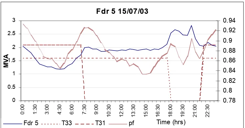
Figure 13 - Graph of the Winter Load on Substation 1 Feeder 5

4.3.8

Substation 1 Industrial Feeder Summary

Load:

In Figure 13 and Figure 14 the base load for both the winter and summer periods is similar in appearance, however the day peak in summer is approximately 200% of the winter load. This would possibly be attributed primarily to air-conditioning load, also the tariff control does not make any difference to the load profile.

Power Factor:

The power factor in both summer (Figure 14) and winter (Figure 13) is relatively consistent, however in both cases the power factor gets to a low level, ie. near 0.8.

Fdr 5 15/07/03

0 0.5 1 1.5 2 2.5 3

0:00 1:30 3:00 4:30 6:00 7:30 9:00 _10:30 _12:00 _13:30 _15:00 _16:30 _18:00 _19:30 _21:00 _22:30

Time (hrs)

MV

A

0.76

0.78

0.8

0.82

0.84

0.86

0.88

0.9

Fdr 5 T33 T31 pf

Fdr 5 09/12/03

0.0 1.0 2.0 3.0 4.0 5.0 6.0

0:00 1:30 3:00 4:30 6:00 7:30 9:00 _10:30 _12:00 _13:30 _15:00 _16:30 _18:00 _19:30 _21:00 _22:30

Time (hrs)

MV

A

0.76 0.77 0.78 0.79 0.8 0.81 0.82 0.83 0.84 0.85

(42)

4.4

Substation Number 2 Data

4.4.1

Transformers 2 by 20 MVA 66/11kV

Capacitor Bank 1 by 5.4 MVAr @ 12kV

Number of Feeders 6 @ 11kV

Ripple Control Nil

Peak Load 14.75 MVA

Number of Customers 2830

Table 3 - Summary of Substation Number 2 Data

4.4.2

Load growth for Substation Number 2

Figure 15 - Graph of Substation 2 Load Growth for the past 9 years

0 2 4 6 8 10 12 14 16 18 20

Ma

y-96

Oc

t-96

M

ar-97

Aug-97 Jan-98 Jun-98 _Nov-98 Apr-99 Sep-99 Feb-00 Jul

-00

Dec-00 _Ma

y-01

Oc

t-01

M

ar-02

Aug-02 Jan-03 Jun-03 _Nov-03 Apr-04

MW

0% 10% 20% 30% 40% 50% 60% 70% 80% 90% 100% Monthly Max Demand (MW) - Substation 2 - Sub Total

LF

(43)

4.4.3

Substation Number 2 Transformer Load Summary

[image:43.595.118.501.92.294.2]

Figure 16 - Graph of the Total Winter Load on Substation 2

4.4.4

Substation 2 Transformer Summary

Load:

This substation has had a significant decrease in load over the past few years, this has been solely to the closing of a large industrial enterprise that was being supplied from the substation. This substation has a similar issue with the substation 1 with the two peaks in the winter load (Figure 16). In Figure 17 the load on this substation indicates a heavy air-conditioning load progressively ramping up as the ambient temperature gets hotter throughout the day. The power factor for this substation is relatively stable most of the time, however in winter as the load increases so does the power factor indicating that the load is becoming more resistive.

T31

T33

Sub 2 - Transformer 15/07/03

0 1 2 3 4 5 6 7

0:00 1:30 3:00 4:30 6:00 7:30 9:00 _10:30 _12:00 _13:30 _15:00 _16:30 _18:00 _19:30 _21:00 _22:30

Time (hrs) MV A 0.88 0.9 0.92 0.94 0.96 0.98 1

TFR Load T33 T31 pf

Sub 2 - Transformer 09/12/03

0 1 2 3 4 5 6 7 8 9

0:00 1:30 3:00 4:30 6:00 7:30 9:00 _10:30 _12:00 _13:30 _15:00 _16:30 _18:00 _19:30 _21:00 _22:30

Time (hrs) MV A 0.84 0.86 0.88 0.9 0.92 0.94 0.96

(44)

4.4.5

Substation Number 2 Example of Domestic Feeder

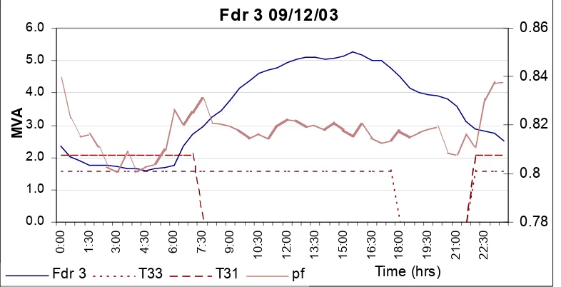
Figure 18 - Graph of the Winter Load on Substation 2 Feeder 3

4.4.6

Substation 2 Domestic Feeder Summary

Load:

In Figure 18 the load peaks around the 6pm mark which appear to be hotwater peaks. Also in Figure 19 the summer load ramps from 6am to 8pm with a 500kVA rise between 6pm and 8pm.

Power Factor:

Changes in the power factor during winter (Figure 18) followed the load this is probably due to the changing proportions of resistive and reactive load. As more resistive load

Fdr 3 15/07/03

0 0.5 1 1.5 2 2.5 3 3.5

0:00 1:30 3:00 4:30 6:00 7:30 9:00 _10:30 _12:00 _13:30 _15:00 _16:30 _18:00 _19:30 _21:00 _22:30

Time (hrs)

MV

A

0.82 0.84 0.86 0.88 0.9 0.92 0.94 0.96 0.98

Fdr 3 T33 T31 pf

Fdr 3 09/12/03

0.0 0.5 1.0 1.5 2.0 2.5 3.0 3.5 4.0

0:00 1:30 3:00 4:30 6:00 7:30 9:00 _10:30 _12:00 _13:30 _15:00 _16:30 _18:00 _19:30 _21:00 _22:30

Time (hrs)

MV

A

0.82 0.84 0.86 0.88 0.9 0.92 0.94 0.96

(45)

4.4.7

Figure 20 - Graph of the Winter Load on Substation 2 Feeder 4

4.4.8

Substation 2 Industrial Feeder Summary

Load:

In Figure 20 and Figure 21 the summer and winter peaks for this feeder are almost identical.

Power Factor:

In Figure 20 and Figure 21 there is no problem with the power factor on this feeder.

Fdr 4 09/12/03

0.0 0.5 1.0 1.5 2.0 2.5

0:00 1:30 3:00 4:30 6:00 7:30 9:00 _10:30 _12:00 _13:30 _15:00 _16:30 _18:00 _19:30 _21:00 _22:30

Time (hrs) MV A 0.7 0.75 0.8 0.85 0.9 0.95 1

Fdr 4 T33 T31 pf

Fdr 4 15/07/03

0 0.5 1 1.5 2 2.5 0: 00 1: 30 3: 00 4: 30 6: 00 7: 30 9: 00 10: 30 12: 00 13: 30 15: 00 16: 30 18: 00 19: 30 21: 00 22: 30 Time (hrs) MVA 0.76 0.8 0.84 0.88 0.92 0.96 1

(46)

4.5

4.5.1

Transformers 2 x 100MVA 132/66kV 2 x 20MVA 66/11kV

Capacitor Bank 1 x 24MVar

Number of Feeders 8 x 11kV

Ripple Control Yes

Peak Load 30.78 MVA

Table 4 - Summary of Substation Number 3 Data

4.5.2

Load growth for Substation Number 3

Figure 22 - Graph of Substation 3 Load Growth for the past 9 years

0 5 10 15 20 25 30 35 40 Jul-9 6

Dec-96May-97Oct-9 7 Mar-9

8

Aug-98

Jan-99Jun-99Nov-99Apr-00Sep-0 0 Feb-0 1 Jul-0 1 Dec-0 1 May-02Oct-0

2 Mar-0

3

Aug-03 Jan-04Jun-04

LF

(47)

4.5.3

Substation Number 3 Transformer Load Summary

Figure 23 - Graph of the Total Winter Load on Substation 3

4.5.4

Substation 3 Transformer Summary

Load:

Figure 23 again shows the load peaks around the 6pm – 8pm timeframe, this also indicates that a review is required on the hotwater switching times. In Figure 24 there is not much that can be done unless better demand-side management practices are employed.

Power Factor:

Whilst the power factor in both Figure 23 and Figure 24 appears erratic it only has a narrow bandwidth, however power factor correction may make some difference to the overall load.

T31

T33

Sub 3 - Transformer 15/07/03

0 2 4 6 8 10 12 14 16 18 20

0:00 1:30 3:00 4:30 6:00 7:30 9:00 _10:30 _12:00 _13:30 _15:00 _16:30 _18:00 _19:30 _21:00 _22:30

Time (hrs) MV A 0.76 0.78 0.8 0.82 0.84 0.86 0.88 0.9 0.92

TFR Load T33 T31 pf

Sub 3 - Transformer 09/12/03

0 5 10 15 20 25 30

0:00 1:30 3:00 4:30 6:00 7:30 9:00 _10:30 _12:00 _13:30 _15:00 _16:30 _18:00 _19:30 _21:00 _22:30

Time (hrs) MV A 0.78 0.8 0.82 0.84 0.86 0.88

(48)

4.5.5

[image:48.595.116.506.88.292.2]

Figure 25 - Graph of the Winter Load on Substation 3 Feeder 5

4.5.6

Substation 3 Domestic Feeder Summary

Load:

The winter load in Figure 25 indicates that some work may be required on the hotwater switching times. Also Figure 26 is exceeding the feeder design limit for summer and will need load moved or upgrading.

Power Factor:

As can be seen in Figure 25 and Figure 26 the power factor is relatively stable

Fdr 5 15/07/03

0 0.5 1 1.5 2 2.5 3

0:00 1:30 3:00 4:30 6:00 7:30 9:00 _10:30 _12:00 _13:30 _15:00 _16:30 _18:00 _19:30 _21:00 _22:30

Time (hrs)

MV

A

0.78 0.8 0.82 0.84 0.86 0.88 0.9 0.92 0.94

Fdr 5 T33 T31 pf

Fdr 5 09/12/03

0.0 0.5 1.0 1.5 2.0 2.5 3.0 3.5 4.0 4.5

0:00 1:30 3:00 4:30 6:00 7:30 9:00 _10:30 _12:00 _13:30 _15:00 _16:30 _18:00 _19:30 _21:00 _22:30

Time (hrs)

MV

A

0.78 0.8 0.82 0.84 0.86 0.88 0.9

(49)

[image:49.595.119.512.321.522.2]

4.5.7

Figure 27 - Graph of the Winter Load on Substation 3 Feeder 3

4.5.8

Substation 3 Industrial Feeder Summary

Load:

There is a 2MVA difference between winter (Figure 27) and summer (Figure 28), otherwise this feeder exhibits the typical industrial characteristics.

Power Factor:

For both winter (Figure 27) and summer (Figure 28) the power factor is around 0.82-0.84 and it is stable. There would be savings and advantages by improving the power factor to around 0.9.

Fdr 3 15/07/03

0 0.5 1 1.5 2 2.5 3 3.5 0: 00 1: 30 3: 00 4: 30 6: 00 7: 30 9: 00 10: 30 12: 00 13: 30 15: 00 16: 30 18: 00 19: 30 21: 00 22: 30 Time (hrs) MVA 0.8 0.82 0.84 0.86 0.88 0.9

Fdr 3 T33 T31 pf

Fdr 3 09/12/03

0.0 1.0 2.0 3.0 4.0 5.0 6.0

0:00 1:30 3:00 4:30 6:00 7:30 9:00 _10:30 _12:00 _13:30 _15:00 _16:30 _18:00 _19:30 _21:00 _22:30

Time (hrs) MV A 0.78 0.8 0.82 0.84 0.86

(50)

4.6

4.6.1

Transformers 2 x 20MVA 66/11kV

Capacitor Bank 1 x 5.4MVar at 12kV

Ripple Control Nil

Peak Load 19.86 MVA

[image:50.595.119.519.397.625.2]

Table 5 - Summary of Substation Number 4 Data

4.6.2

Load growth for Substation Number 4

Figure 29 - Graph of Substation 4 Load Growth for the past 14 years

0 5 10 15 20 25 30

Aug-91 Mar-92 Oc

t-92

Ma

y-93

Dec-93 Jul

-94

Feb-95 Sep-95 Apr-96 Nov-96 Jun-97 Jan-98 Aug-98 Mar-99 Oc

t-99

Ma

y-00

Dec-00 Jul

-01

Feb-02 Sep-02 Apr-03 Nov-03 Jun-04

LF

(51)

[image:51.595.118.507.94.295.2]

4.6.3

Substation Number 4 Transformer Load Summary

[image:51.595.119.512.335.537.2]

Figure 30 - Graph of the Total Winter Load on Substation 4

4.6.4

Substation 4 Transformer Summary

Load:

The winter load in Figure 30 has a morning peak around 9am. The summer load in Figure 31 indicates that better demand-side management practices could make a difference to the overall load profile.

Power Factor:

The power factor for both Figure 30 and Figure 31 is good and stable. T33

Sub 4 - Transformer 15/07/03

0 2 4 6 8 10 12

0:00 1:30 3:00 4:30 6:00 7:30 9:00 _10:30 _12:00 _13:30 _15:00 _16:30 _18:00 _19:30 _21:00 _22:30

Time (hrs)

MV

A

0.94 0.96 0.98 1 1.02

TFR Load T33 T31 pf

Sub 4 - Transformer 09/12/03

0 2 4 6 8 10 12 14 16 18

0:00 1:30 3:00 4:30 6:00 7:30 9:00 _10:30 _12:00 _13:30 _15:00 _16:30 _18:00 _19:30 _21:00 _22:30

Time (hrs)

MV

A

0.94 0.96 0.98 1 1.02

(52)

[image:52.595.115.510.90.292.2]

4.6.5

Figure 32 - Graph of the Winter Load on Substation 4 Feeder 1

4.6.6

Substation 4 Domestic Feeder Summary

Load:

The winter load in Figure 32 again shows a peak between 6pm and 8pm. The summer load in Figure 33 has a steady ramp up possibly due to air-conditioning load, until an outage at about 10pm.

Power Factor:

Except for the outage at 10pm the power factor for both Figure 32 and Figure 33 is stable.

Fdr 1 15/07/03

0 0.5 1 1.5 2 2.5

0:00 1:30 3:00 4:30 6:00 7:30 9:00 _10:30 _12:00 _13:30 _15:00 _16:30 _18:00 _19:30 _21:00 _22:30

Time (hrs)

MV

A

0.8 0.82 0.84 0.86 0.88 0.9 0.92 0.94 0.96 0.98 1

Fdr 1 T33 T31 pf

Fdr 1 09/12/03

0.0 0.5 1.0 1.5 2.0 2.5 3.0

0:00 1:30 3:00 4:30 6:00 7:30 9:00 _10:30 _12:00 _13:30 _15:00 _16:30 _18:00 _19:30 _21:00 _22:30

Time (hrs)

MV

A

0.8 0.82 0.84 0.86 0.88 0.9 0.92 0.94 0.96

[image:52.595.118.512.332.533.2]

(53)

[image:53.595.116.509.83.290.2]

4.6.7

Figure 34 - Graph of the Winter Load on Substation 4 Feeder 7

4.6.8

Substation 4 Industrial Feeder Summary

Load:

There is very little load variation for both the winter (Figure 34) and summer

(Figure 35) loads.

Power Factor:

The power factor for both winter (Figure 34) and summer (Figure 35) is

stable, however further investigation is required to determine why this feeder has a low

power factor near 0.7.

Fdr 7 15/07/03

0 0.5 1 1.5 2 2.5

0:00 1:30 3:00 4:30 6:00 7:30 9:00 _10:30 _12:00 _13:30 _15:00 _16:30 _18:00 _19:30 _21:00 _22:30

Time (hrs)

MV

A

0.7 0.72 0.74 0.76 0.78

Fdr 7 T33 T31 pf

Fdr 7 09/12/03

0.0 0.5 1.0 1.5 2.0 2.5

0:00 1:30 3:00 4:30 6:00 7:30 9:00 _10:30 _12:00 _13:30 _15:00 _16:30 _18:00 _19:30 _21:00 _22:30

Time (hrs)

MV

A

0.66 0.68 0.7 0.72 0.74 0.76 0.78

[image:53.595.117.510.327.529.2]

(54)

4.7

Substation Number 5 Data

4.7.1

Capacitor Bank Nil

Ripple Control Nil

Peak Load 8.63MVA

[image:54.595.112.519.407.629.2]

Table 6 - Summary of Substation Number 5 Data

4.7.2

Load growth for Substation Number 5

Figure 36 - Graph of Substation 5 Load Growth for the past 13 years

0 1 2 3 4 5 6 7 8 9 10

M

ar-92

Sep-92 Apr-93 _Nov-93 Jun-94 Jan-95 Aug-95 Mar-96 Oc

t-96

Ma

y-97

Dec-97 Jul

-98

Feb-99 Sep-99 Apr-00 _Nov-00 Jun-01 Jan-02 Aug-02 Mar-03 Oc

t-03

Ma

y-04

LF

(55)

[image:55.595.118.508.93.295.2]

4.7.3

Substation Number 5 Transformer Load Summary

Figure 37 - Graph of the Total Winter Load on Substation 5

4.7.4

Substation 5 Transformer Summary

Load:

In Figure 37 and Figure 38 there is a 6am peak that will require further investigation, although it is prevalent in both summer and winter it indicates that there maybe an industrial load that needs to be to start and finish approximately a half an hour earlier.

Power Factor:

The power factor for both winter (Figure 37) and summer (Figure 38) is good and stays above 0.9, almost reaching unity.

T33

Sub 5 - Transformer 15/07/03

0 1 2 3 4 5 6

0:00 1:30 3:00 4:30 6:00 7:30 9:00 _10:30 _12:00 _13:30 _15:00 _16:30 _18:00 _19:30 _21:00 _22:30

Time (hrs)

MV

A

0.88 0.9 0.92 0.94 0.96 0.98 1

TFR Load T33 T31 pf

Sub 5 - Transformer 09/12/03

0 1 2 3 4 5 6

0:00 1:30 3:00 4:30 6:00 7:30 9:00 _10:30 _12:00 _13:30 _15:00 _16:30 _18:00 _19:30 _21:00 _22:30

Time (hrs)

MV

A

0.86 0.88 0.9 0.92 0.94 0.96 0.98

[image:55.595.117.506.334.537.2]

(56)

4.7.5

[image:56.595.116.509.87.289.2]

Figure 39 - Graph of the Winter Load on Substation 5 Feeder 1

4.7.6

Substation 5 Domestic Feeder Summary

Load:

The winter load (Figure 39) peaks between 6pm and 8pm need further investigation. However the winter peak is larger than the summer (Figure 40) peak, even though there is an outage at approximately 10pm.

Power Factor:

The power factor in both Figure 39 and Figure 40 is good and stable.

Fdr 1 15/07/03

0 0.2 0.4 0.6 0.8 1 1.2 1.4 1.6 1.8

0:00 1:30 3:00 4:30 6:00 7:30 9:00 _10:30 _12:00 _13:30 _15:00 _16:30 _18:00 _19:30 _21:00 _22:30

Time (hrs)

MV

A

0.94 0.96 0.98 1 1.02

Fdr 1 T33 T31 pf

Fdr 1 09/12/03

0.0 0.5 1.0 1.5 2.0 0: 00 1: 30 3: 00 4: 30 6: 00 7: 30 9: 00 10: 30 12: 00 13: 30 15: 00 16: 30 18: 00 19: 30 21: 00 22: 30 Time (hrs) MVA 0.9 0.92 0.94 0.96 0.98 1

(57)

4.7.7

Figure 41 - Graph of the Winter Load on Substation 5 Feeder 3

4.7.8

Substation 5 Industrial Feeder Summary

Load:

Figure 40 and Figure 41 depicts a feeder that has a dedicated pumping load that utilises off peak times to pump water. This feeder combined with a typical industrially loaded substation would possibly make an ideal feeder.

Power Factor:

The power factor in both Figure 40 and Figure 41 is typical of a dedicated pumping load with motor starting not being detected due to the fact that the data is read in 15 minute intervals.

Fdr 3 15/07/03

0 0.5 1 1.5 2 2.5

0:00 1:30 3:00 4:30 6:00 7:30 9:00 _10:30 _12:00 _13:30 _15:00 _16:30 _18:00 _19:30 _21:00 _22:30

Time (hrs)

MV

A

0.75 0.8 0.85 0.9 0.95 1 1.05

Fdr 3 T33 T31 pf

Fdr 3 09/12/03

0.0 0.5 1.0 1.5 2.0 2.5

0:00 1:30 3:00 4:30 6:00 7:30 9:00 _10:30 _12:00 _13:30 _15:00 _16:30 _18:00 _19:30 _21:00 _22:30

Time (hrs)

MV

A

0.86 0.9 0.94 0.98 1.02

(58)

4.8

4.8.1

Capacitor Bank 1 x 5.4MVar at 12kV

Ripple Control Nil

Peak Load 20.78 MVA

[image:58.595.116.516.389.620.2]

Table 7- Summary of Substation Number 6 Data

4.8.2

Load growth for Substation Number 6

Figure 43- Graph of Load Growth for 13 years for Substation 6

0 5 10 15 20 25 30

Jul

-91

Feb-92 Sep-92 Apr-93 Nov-93 Jun-94 Jan-95 Aug-95 Mar-96 Oc

t-96

Apr-97 _Nov-97 Jun-98 Jan-99 _Aug-99 _Mar-00 _Sep-00 Apr-01 _Nov-01 Jun-02 Jan-03 _Aug-03 _Mar-04

LF

(59)

4.8.3

Substation Number 6 Transformer Load Summary

Figure 44 - Graph of the Total Winter Load on Substation 6

4.8.4

Substation 6 Transformer Summary

Load:

Figure 44 shows that the winter load peaks between 6pm and 8pm, this needs further investigation. The summer load in Figure 45 is approximately 6MVA higher than the winter peak, this is possibly due to air-conditioner load.

Power Factor:

The power factor in Figure 44 and Figure 45 remains above 0.9 and is stable.

Sub 6 - Transformer 15/07/03

0 2 4 6 8 10 12 14 0: 00 1: 30 3: 00 4: 30 6: 00 7: 30 9: 00 10: 30 12: 00 13: 30 15: 00 16: 30 18: 00 19: 30 21: 00 22: 30 Time (hrs) MVA 0.9 0.92 0.94 0.96 0.98 1

TFR Load T33 T31 pf

Sub 6 - Transformer 09/12/03

<