Performance of preliminary test estimator under linex loss function

Performance of Preliminary Test Estimator under Linex Loss Function

Zahirul Hoque, Shahjahan Khan1 _{and Jacek Wesolowski}2 Department of Statistics

UAE University

P.O. Box 17555, Al Ain UAE

[email protected]

Key Words: Linex loss; non-sample prior information; unrestricted estimator; pre-liminary test estimator; risk function.

ABSTRACT

This paper studies the performance of the unrestricted estimator (UE) and pre-liminary test estimator (PTE) of the slope parameter of simple linear regression model under linex loss function. The risk functions of both the UE and PTE are derived. The moment generating function (MGF) of the PTE is derived which turns out to be a component of the risk function. From the MGF the first two moments of the PTE are obtained and found to be identical to that obtained by using a different approach in Khanet al. (2002). The performance of the PTE is compared with that of the UE by using the analytical and graphical as well as the numerical methods. It is revealed that if the uncertain non-sample prior information about the value of the slope is not too far from its true value then the PTE outperforms the UE.

1

INTRODUCTION

The squared error loss (SEL) function is one of the most widely used loss func-tions in decision theory. The popularity of this symmetric loss function is due to its mathematical and interpretational convenience. Due to the symmetric nature it fails to differentiate between overestimation and underestimation of any

parame-1_{University of Southern Queensland, Australia}

ter. The criticism against the appropriateness of the SEL is ever growing since the introduction of the asymmetric linex loss (LL) by Varian (1975).

The LL function for estimating any parameter θ by θ∗_{, is given by L(δ) =}

b

exp(aδ)₋aδ ₋1

∀ a ₆= 0, b > 0 where δ is the estimation error. The two

parameters a and b in L(δ) serve to determine the shape and scale, respectively, of L(δ). A positive a indicates that overestimation is more serious than underestima-tion and a negative a represents the reverse situation. The magnitude of a reflects the degree of asymmetry about δ = 0. If a _→ 0, then the LL reduces to the SEL. Without any loss of generality it can be assumed that b= 0. Further details about the properties of this loss function are available in Varian (1975), Zellner (1986), Parsian and Kirmani (2002) and Parsian and Farispour (1993).

The exclusive sample information based UE of slope parameter is uniformly min-imum variance unbiased estimator. The natural expectation is that the use of addi-tional information such as non-sample prior information with the sample information would result in a better estimator than UE. Based on both sample and non-sample prior information, Bancroft (1944) pioneered the idea of PTE and showed that with respect to SEL function it outperforms UE under certain conditions.

The main purpose of this paper is to investigate the performance of the PTE of the slope parameter of simple linear regression model under the LL function. The risk of both the UE and PTE have been derived. The MGF of the PTE is also derived in this paper. The performance of the PTE relative to that of the UE is compared. It is revealed that if the non-sample prior information about the value of the slope is not too far from its true value the PTE outperforms the UE. Otherwise, none of the estimators outperforms the other.

2

THE MODEL AND PRELIMINARIES

Consider a set ofnrandom sample observationsyi fori= 1,2, . . . , nfrom the simple

linear regression model

y=β0+β1x+ε (1)

where y is the response variable, β0 is the intercept parameter, β1 is the slope parameter,x is the predictor andε is the error component. Assume that the errors are independently and identically distributed as a normal variable with mean 0 and variance σ2_{. In conventional notation we write ε iid N(0, σ}2_).

Combining sample and non-sample prior information Bancroft (1944), and later Han and Bancroft (1968), developed the preliminary test estimator (PTE) for any unknown parameter. The risk properties of this estimator, under SEL, is investi-gated by many authors, see for instance, Khan and Saleh (2001); Khanet al. (2002). Giles and Giles (1992) studied the performance of the PTE of the error variance after a pre-test of exact linear restrictions on the regression coefficients in multiple regression set-up. They compared the risk of this estimator under linex loss with that under SEL. Later Giles and Giles (1996) studied the risk of the error vari-ance under LINEX loss after a pre-test for homoscedasticity of the varivari-ances in the two-sample heteroscedastic linear regression model.

For the linear regression model in equation (1) the exclusively sample information based unrestricted estimator (UE) of β1 is ˜β1 =Sxx−1Sxy whereSxx =Pni=1(xi−x¯)2

andSxy =Pn_i=1(xi−x¯)(yi−y¯). Assume that uncertain non-sample prior information

about the value of the slope is available either from previous study or from practical experience of researchers or experts. Such non-sample prior information can be expressed in the form of the null hypothesis H0 : β1 = β10 which may be true, but there is doubt. The estimator of β1, under the aboveH0, is known as the restricted estimator (RE), and is given by ˆβRE

1 =β10. A simple form of PTE ofβ1 is ˆ

βPTE

1 = ˜β1−( ˜β1−βˆ RE

1 )I(F1, ν < F1, ν(α)) (2)

where I(A) is an indicator function of the set A and F1,ν(α) is the upper α-level

to test the null hypothesis presented earlier. Under the alternative hypothesis,

Ha : β1 6= β10 the distribution of F is a non-central F with (1, ν) d.f. and non-centrality parameter ∆2 _{where ∆ =}√_S

xx(β1−β10)σ−1.

Under the SEL the PTE outperforms both the UE and RE in the neighborhood of ∆2 _{= 0, see for instance Khan and Saleh (2001). As ∆}2 _{deviates further from 0,} the performance of the PTE becomes worse than those of the UE and RE. However, as ∆2 _{approaches a very large value the performance of the PTE becomes the same} as that of the UE. On the other hand, as ∆2 _{increases from zero, the performance of} the RE worsen. Therefore, with respect to SEL the PTE is regarded as an improved estimator if the value of ∆2 _{is not too far from zero. However, due to the growing} criticism against SEL, it is of interest to investigate the performance of the PTE under the asymmetric losses such as LL.

3

THE RISK OF UE AND PTE OF THE SLOPE

The following lemma is useful for the derivation of the risk functions of the UE and PTE.

Lemma 3.1 If Z _∼N(0,1), andZ and S_∼χ2

k are independent then for any Borel

measurable function φ :_{< ×}(0,_∞)_{→ <} and for any c_{∈ <},

E[exp(cZ)φ(Z, S)] = exp(c2/2) E [φ(Z+c, S)] (3) provided (exp(cZ)φ(Z, S))is integrable.

Proof. By definition

E[exp(cZ)φ(Z, S)] = E[E [exp(cZ)φ(Z, S)_|S]] = E

1 √

2π

Z

<

φ(z, S) exp(cz₋z2/2)dz

= exp(c2/2) E

1 √

2π

Z

<

φ(z, S) exp(₋1

2(z−c) 2_)dz

.

Consider U =Z₋c. The Jacobian of the transformation is _|J_|= 1. Therefore, E[exp(cZ)φ(Z, S)] = exp(c2/2) E [φ(Z+c, S)].

Theorem 3.2 The risk of the UE of β1 under the LL function is given by

Rhβ˜1;β

i

= exp(a2

1/2)−1 where a1 =aσ/√Sxx.

Proof. By definition, the risk function of the UE of β1 under the LL is

Rhβ˜1;β1

i

= Ehexp(a( ˜β1−β1))

i

−aEhβ˜1−β1

i

−1. (4)

The first component of the right hand side of (4) is Ehexp(a( ˜β1−β1))

i

= E[exp(a1Z)] (5)

where a1 =aσ/√Sxx and Z =√Sxx(β1 −β10)σ−1 ∼N(0, 1). Applying Lemma 3.1 to (5) with φ as identity, we get

Ehexp(a( ˜β1−β1))

i

= exp(a2₁/2). (6)

As ˜β1 is unbiased, the second component of the right hand side of (4) is 0 . Collecting the results from (6) and substituting in (4), the expression of the risk function of the UE of β1 is obtained.

The following two lemmas are essential to derive the risk function of the PTE.

Lemma 3.3 IfX follows a non-central Student’st distribution withk d.f. and

non-centrality parameter δ then

ft(k,δ)(x) +ft(k,δ)(−x) = 2x fF(1, k, δ2)(x2) ∀ x >0 (7) where ft(k,δ)(·) is the density function of a non-central Student’s t distribution with

k d.f. and non-centrality parameter δ, and fF(1, k, δ2₎(·) is the density function of a non-central F distribution with (1, k) d.f. and non-centrality parameter δ2_.

Proof. The density function of the non-central Student’st distribution withk d.f.

and non-centrality parameterδ is given by

ft(k, δ)(x) =

kk/2_exp(−δ2_/2) Γ(k/2)√π(k+x2₎k+12

∞

X

i=0 Γ

k+ 1 +i

2

(xδ)i i!

2

k+x2

i/2

Consider now ft(k,δ)(x) +ft(k,δ)(−x) for any arbitrary x ≥ 0. Then (8) implies

that the terms of the series with odd powers of x cancel and the terms with even powers of x are duplicated. Thus,

ft(k,δ)(x) +ft(k,δ)(−x) =

2kk/2_exp(−δ2_/2) Γ(k/2)√π(k+x2₎k+12

∞

X

i=0 Γ

k+ 1

2 +i

x2i_δ2i

(2i)!

2

k+x2

i

= 2k

k/2_exp(−δ2_/2) Γ(k/2)√π(k+x2₎k+12

∞

X

i=0 Γ

k+ 1

2 +i

(x2₎i_(δ2₎i 2i_{i! (2i−1)!!}

2i

(k+x2₎i

= 2xk

k/2_exp(−δ2_/2)(x2₎−1/2 Γ(k/2)(k+x2₎k+12

∞

X

i=0

Γ k+1 2 +i

i! Γ(1 2 +i)

x2_δ2 2(k+x2₎

i

= 2x fF(1, k, δ2)(x2). This completes the proof of the lemma.

Lemma 3.4 For any two positive integers m and n

∂fF(m, n, D)(x)

∂D =−

1

2fF(m, n, D)(x) +

m

2(m+ 2)fF(m+2, n, D)

mx

m+ 2

, x, D_∈[0, _∞)

where fF(l,n,D)(·) denotes the density function of a non-central F distribution with

(l, n) d.f. and non-centrality parameter D.

Proof. The density function of the non-centralF with (m, n) d.f. and non-centrality

parameter D is given by

fF(m,n,D)(x) =

exp(₋D/2)mm/2_nn/2 Γ(n/2)

xm2−1 (n+mx)m+2n

∞

X

j=0

mxD

2(n+mx)

j

Γ m+₂n+j

Γ m

2 +j

j!. Differentiating both sides with respect to D, we get

∂fF(m, n, D)(x)

∂D =−

1

2fF(m,n,D)(x) +

exp(₋D/2)mm/2_nn/2 Γ(n/2)

xm/2−1 (n+mx)m+2n × ∞ X j=1 mx

2(n+mx)

j

Dj−1 (j₋1)!

Γ m+₂n +j

Γ m

2 +j

=₋1

2fF(m,n,D)(x) +

exp(₋D/2)mm/2_nn/2 Γ(n/2)

xm/2−1 (n+mx)m+2n × ∞ X i=0 mx

2(n+mx)

i+1

Di i!

Γ m+2+₂ n+i

Γ m+2 2 +i

=₋1

2fF(m,n,D)(x) +

exp(₋D/2)mm/2+1_nn/2 2 Γ(n/2)

xm2+2−1 (n+mx)m+2+2 n × ∞ X i=0 mxD

2(n+mx)

i_Γ m+2+n

2 +i

i! Γ m+2 2 +i

=₋1

2fF(m,n,D)(x) +

exp(₋D/2)mm2+2nn/2 2Γ(n/2)

mx m+2

m₂+2−1 _m+2

m

m/2

n+ (m+ 2)_mmx₊₂

m+2+n

2 × ∞ X i=0 "

(m+ 2)mxD m+2 2

n+ (m+ 2) mx

m+2

#i

Γ m+2+₂ n+i

i! Γ m+2 2 +i

=₋1

2fF(m, n, D)(x) +

mexp(₋D/2)(m+ 2)m2+2nn/2 mx

m+2

m+2 2 −1

2(m+ 2)Γ(n/2)

n+ (m+ 2)_mmx₊₂

m+2+n

2 × ∞ X i=0 "

(m+ 2)_mmx₊₂D

2

n+ (m+ 2)_mmx₊₂

#i

Γ m+2+n

2 +i

i! Γ m₂+2 +i

=₋1

2fF(m, n, D)(x) +

m

2(m+ 2)fF(m+2, n, D)

mx

m+ 2

.

This completes the proof of the lemma.

Theorem 3.5 The risk function of the preliminary test estimator of the slope

pa-rameter β1 under the LL function is given by

RhβˆPTE 1 ;β1

i

= exp(₋a1∆)G1, ν c; ∆2

+ exp(a2₁/2)

1₋G1, ν c; (∆ +a1)2

+a1∆G3, ν(c/3; ∆2)−1 (9)

where c=F1,ν(α) and Ga, ν(q; θ) is the cdf of non-central F distribution with (a, ν)

d.f., non-centrality parameter θ and evaluated at q.

Proof. By definition, the risk function of the PTE of β1 under the LL function is

RhβˆPTE 1 ;β1

i

= E[exp(aΦ)]₋aE[Φ]₋1 (10) where Φ = ˆβPTE

1 −β1.

The first component of the right hand side of (10) is E[exp(aΦ)] = E

exp(a_{( ˜β1−β1)−( ˜β1−β10)I(F1, ν < F1, ν(α))})

×

I(F1, ν < F1, ν(α)) +I(F1, ν ≥F1, ν(α))

= exp(a(β10−β1))P(F1, ν < c) + E

exp(a( ˜β1−β1))I(F1, ν ≥c)

(11)

The first component of the right hand side of (11) is

exp(a(β10−β1))P(F1, ν < c) = exp(−a1∆)G1, ν(c; ∆2). (12)

The second component of the right hand side of (11) can be written as E

exp(a( ˜β1−β1))I(F1, ν ≥c)

= E

exp(a1Z)I

(Z + ∆)2

νS2

n/σ2 ≥ c

(13) where a1 = √aσ_Sxx, Z ∼N(0,1) and (νS

2

n/σ2)∼χ2ν. Z and Sn are independent.

Applying Lemma 3.1 to (13) with φ(X, Y) =I(X+∆)_Y 2 _≥c we get

Ehexp(a( ˜β1−β1))I(F1, ν ≥c)

i

= exp(a2₁/2)

1₋G1, ν c; (∆ +a1)2

. (14)

Combining (12) and (14) the first component of the right hand side of (10) yields E[exp(aΦ)] = exp(₋a1∆)G1, ν c; ∆2

+ exp(a2₁/2)

1₋G1, ν c; (∆ +a1)2

. (15)

From (15) the moment generating function of the PTE of β1 is

m(a) = exp(₋a1∆)

Z 0

−c

ft(ν,∆)(x)dx+

Z c

0

ft(ν,∆)(x)dx

+ exp(a2₁/2)

1₋

Z 0

−c

ft(ν,∆−a1)(x)dx−

Z c

0

ft(ν,∆−a1)(x)dx

. (16)

Writing gt(ν,∆)(x) =ft(ν,∆)(x) +ft(ν,∆)(−x) for any x >0 in (16) we get

m(a) = exp(₋a1∆)

Z c

0

gt(ν,∆)(x)dx+ exp(a21/2)

Z ∞

c

gt(ν,∆−a1)(x)dx . (17) Applying Lemma 3.3 in (17) we get

m(a) = exp(₋a1∆)

Z c

0

fF(1, ν,∆2)(y)dy+ exp(a2 1/2)

Z ∞

c

fF(1, ν,(−∆−a1)2)(y)dy . Differentiating both sides of the above equation with respect to a, then using Lemma 3.4 and finally changing the variable y/3 to t in the left integral we get

m0_{(a) = √}σ

Sxx

h

−∆ exp(₋a1∆)

Z c

0

fF(1, ν,∆2₎(y)dy+a₁exp(a2 1/2) ×

Z ∞

c

fF(1, ν,(∆+a1)2)(y)dy−(∆ +a1) exp(a2 1/2)

Z ∞

c

fF(1, ν,(∆+a1)2)(y)dy + (∆ +a1) exp(a21/2)

Z ∞

c/3

fF(3, ν,(∆+a1)2)(y)dy

i

Putting a = 0 in (18) we get E(Φ) = ₋(β1−β10)G3, ν(c/3; ∆2) which is the bias

function or equivalently the first moments of the PTE of β1. Therefore, the second component of the right hand side of (10) is

aE[Φ] =₋a1∆G3, ν c/3; ∆2

. (19)

Collecting the expressions from (15) and (19) and plugging into (10) the risk function of the PTE of β1 under the LL function is obtained.This completes the proof of the theorem.

Differentiating both sides of (18) with respect to a, then using using Lemma 3.4 and finally putting a= 0 the mse function of the PTE of β1 is obtained as

MhβˆPTE 1 ;β1

i

=S−1

xxσ2[1−G3, ν(c/3; ∆2) + ∆2{2G3,ν(c/3; ∆2)−G5, ν(c/5; ∆2)}].

For an equivalent expression of the mse function of the shrinkage preliminary test estimator of β1 readers may see Khan et al. (2002). Similarly putting a = 0 in the

mth order derivative of (16) the mth moment of the PTE can be obtained.

4

PERFORMANCE ANALYSIS

For any non-zero value of ∆, the risk function of the PTE of β1 can be written as RhβˆPTE

1 ;β1

i

= Rhβ˜1;β1

i

+g(∆) (20)

where g(∆) = exp(₋a1∆)G1, ν(c; ∆2) +a1∆G3, ν(c/3; ∆2) − exp(a21/2)G1, ν c; (∆

+a1)2

. Therefore, the efficiency of the PTE relative to the UE can be written as EffhβˆPTE

1 ; ˜β1

i

=

exp(a2₁/2)₋1 exp(a2₁/2)₋1 +g(∆)−1

. (21)

Under the null hypothesis, ∆ = 0 and hence

g(∆) =G1,ν(c; 0)−exp(a21/2)G1, ν c;a21

<0 _∀ a₆= 0. (22)

For any positive a, if ∆ is positive a1∆G3, ν(c/3; ∆2) is also positive. Therefore,

for positiveaas ∆ grows larger from 0 efficiency of PTE decreases and crosses the 1-line at ∆ = (exp(a2

1/2)G1, ν(c; (∆ +a1)2)−exp(−a1∆)G1, ν(c; ∆2))/(a1G3, ν(c/3; ∆2))

regardless of the value ofa.

For any negative a, if ∆ is positive a1∆G3, ν(c/3; ∆2) is negative. Therefore, for

negativea, as ∆ grows larger from 0, the efficiency of PTE grows larger, reaching its maximum at some ∆ depending on the magnitude of a, and then starts decreasing and crosses the 1-line for the value of ∆ given above regardless of the value ofa. As

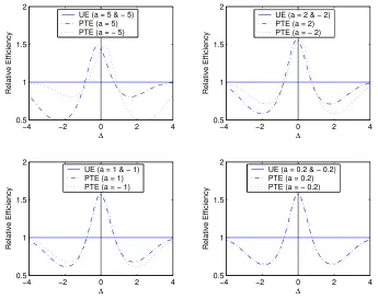
−4 −2 0 2 4

0.5 1 1.5 2

∆

Relative Efficiency

UE (a = 5 & − 5) PTE (a = 5) PTE (a = − 5)

−4 −2 0 2 4

0.5 1 1.5 2

∆

Relative Efficiency

UE (a = 1 & − 1) PTE (a = 1) PTE (a = − 1)

−4 −2 0 2 4

0.5 1 1.5 2

∆

Relative Efficiency

UE (a = 0.2 & − 0.2) PTE (a = 0.2) PTE (a = − 0.2)

−4 −2 0 2 4

0.5 1 1.5 2

∆

Relative Efficiency

UE (a = 2 & − 2) PTE (a = 2) PTE (a = − 2)

Figure 1: Efficiency of PTE relative to UE forα= 0.2,n = 25 and selected a.

∆_{→ ∞}, g(∆) tends to 0, and hence, EffhβˆPTE 1 ; ˜β1

i

→1. Therefore, starting from a certain large ∆, the efficiency of PTE is no different from that of UE.

For very small values of a, the growth pattern of the efficiency of the PTE for both positive and negative values of ∆ are very similar. Because for very small values of a, the LL function reduces to the SEL function.

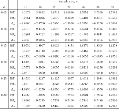
Table 1: Maximum and minimum efficiencies of PTE relative to UE for a= 3

Sample size,n

α 10 15 20 25 30 35 40

0.05 Eff∗ _{4.2674 3.9892 3.8713 3.80640 3.7653 3.7369 3.7162}

Effo 0.2661 0.3076 0.3279 0.3279 0.3401 0.3401 0.3545

∆o −2.6300 −2.4700 −2.3850 −2.3950 −2.3550 −0.3250 −2.3004

0.10 Eff∗ _{2.5615 2.4468 2.3978 2.3706 2.3534 2.3415 2.3328}

Effo 0.3807 0.4202 0.4393 0.4507 0.4585 0.4641 0.4684

∆o −2.3550 −2.2255 −2.1515 −2.1448 −2.1050 −2.1105 −2.0850

0.15 Eff∗ _{1.9556 1.8907 1.8629 1.8474 1.8376 1.8308 1.8258}

Effo 0.4748 0.5112 0.5285 0.5390 0.5462 0.5511 0.5550

∆o −2.1750 −2.0850 −2.0390 −2.0100 −2.0055 −2.0025 −1.9750

0.20 Eff∗ _{1.6429 1.6014 1.5835 1.5736 1.5673 1.5629 1.5597}

Effo 0.5573 0.5900 0.6055 0.6148 0.6211 0.6256 0.6291

∆o −2.0610 −1.9800 −1.9500 −1.9302 −1.9100 −1.9000 −1.8950

0.25 Eff∗ _{1.4530 1.4247 1.4125 1.4057 1.4014 1.3984 1.3962}

Effo 0.6310 0.6597 0.6733 0.6814 0.6868 0.6908 0.6938

∆o −1.9850 −1.9250 −1.8950 −1.8755 −1.8609 −1.8550 −1.8500

0.30 Eff∗ _{1.3268 1.3068 1.2982 1.2934 1.2904 1.2883 1.2867}

Effo 0.6969 0.7215 0.7331 0.7400 0.7446 0.7480 0.7506

∆o −1.925 −1.8650 −1.8459 −1.8255 −1.8100 −1.8080 −1.7968

value ofais determined by the experimenter according to the potential impact of the positive and negative errors of estimation, and the value of ∆ is usually unknown to the experimenter. Regardless of the values ofa and ∆, the efficiency of the PTE is a function ofα. The question is which value ofα should be used for the preliminary test?

Let us consider the efficiency function of the PTE of β1 relative to the UE as a function of α and ∆. Therefore,

EffhβˆPTE 1 ;α,∆

i

=

exp(a2₁/2)₋1 exp(a2₁/2)₋1 +g(∆)−1

. (23)

of the relative efficiency, say Effo, that we are willing to accept. Consider the set

Aα =

α_|EffhβˆPTE 1 ;α,∆

i

≥Effo

for all ∆. An estimator ˆβPTE

1 is chosen which maximizes EffhβˆPTE

1 ;α,∆

i

∀ α_∈Aα and ∆.Thus we solve

maxαmin∆Eff

h

ˆ

βPTE 1 ;α,∆

i

= Effo (24)

for α. The solution provides the maximum and minimum guaranteed efficiencies of the PTE of β1 relative to the UE, for any selected values of n and ∆. Tables 1 presents the maximum guaranteed efficiency (Eff∗) and minimum guaranteed effi-ciency (Eff0) of the PTE ofβ1 relative to the UE, and the value of ∆ (∆o) at which

Eff0 occurs, for selected values ofa,n andα. For example, ifa= 3 andn = 20, and the experimenter wishes to achieve the minimum guaranteed efficiency 0.6055 of the PTE ofβ1, the recommended value ofαis 0.20. This minimum guaranteed efficiency attains at ∆o =−1.95. Fora=−3 the same minimum guaranteed efficiency occurs

at ∆o = 1.95. In general, if a is negative the value of ∆o is positive and vice-versa.

5

CONCLUDING REMARKS

This paper has introduced the computation of any order derivative of the non-central

F distribution with respect to the non-centrality parameter and the derivation of the MGF of the PTE. Moment of the PTE of any order can be obtained from this MGF. For illustration, the bias and mse functions are derived. It is revealed that if the non-sample prior information regarding the value of the parameter is not too far from its true value the PTE outperforms the UE. This result reaffirms the superiority of the PTE under the SEL function. Similar to the shape of the LL function the shape of the risk function of the PTE is also asymmetric. As the value of the shape parameter of the loss function grows smaller the shape of the risk function of the PTE approaches symmetry.

Acknowledgement: The authors acknowledge the useful comments and

References

Bancroft, T.A. (1944) On biases in estimation due to the use of the preliminary test of significance. Ann. Math. Statist., 15, 190-204.

Giles, J.A. and Giles, D.E.A. (1996) Risk of a homoscedasticity pre-test estimator of the regression scale under LINEX loss.J. Stat. Plan. Inf., 50, 21-35.

Giles, J.A. and Giles, D.E.A. (1992) Preliminary-test estimation of the regression scale parameter when the loss function is asymmetric.Comm. Statist., Theo. and Meth., 22(6), 1709-1733.

Han, C.P. and Bancroft, T.A. (1968) On pooling means when variance is unknown. J. Am. Stat. Asso, 63, 133-1342.

Khan, S., Hoque, Z. and Saleh, A.K.Md.E. (2002) Estimation of the slope parame-ter for linear regression model with uncertain prior information. J. Statist. Res.,

36(1), 55-73.

Khan, S. and Saleh, A.K.Md.E. (2001) On the comparison of the pre-test and shrink-age estimators for the univariate normal mean.Statist. Pap., 42(4), 451-473. Parsian, A. and Kirmani, S.N.U.A. (2002) Estimation under LINEX Loss Function.

In Handbook of Applied Econometrics and Statistical Inference, eds. A. Ullah, A.T.K. Wan, and A. Chaturvedi. New York: Marcel Dekker.

Parsian, A. and Farispour, N.S. (1993) On the admissibility and inadmissibility of estimators of scale parameters using an asymmetric loss function,Comm. Statist., Theo. and Meth.,22(10), 2877-2901.

Varian, H.R. (1975) A Bayesian approach to real estate assessment. In Studies in Bayesian Econometrics and Statistics in honor of L.J. Savage, eds., Feinberg and A. Zellner, North Holland, Amsterdam, 195-208.