A Cartesian-grid collocation method
based on radial-basis-function networks
for solving PDEs in irregular domains
N. Mai-Duy
∗and T. Tran-Cong
Faculty of Engineering and Surveying,
The University of Southern Queensland, Toowoomba, QLD 4350, Australia
Submitted to
Numerical Methods for Partial Differential Equations
,
24/4/2006; revised 14/9/2006
Abstract: This paper reports a new Cartesian-grid collocation method based on radial-basis-function networks (RBFNs) for numerically solving elliptic partial differential equa-tions (PDEs) in irregular domains. The domain of interest is embedded in a Cartesian grid, and the governing equation is discretized by using a collocation approach. The new features here are (a) One-dimensional integrated RBFNs are employed to represent the variable along each line of the grid, resulting in a significant improvement of com-putational efficiency, (b) The present method does not require complicated interpolation techniques for the treatment of Dirichlet boundary conditions in order to achieve a high level of accuracy, and (c) Normal derivative boundary conditions are imposed by means of integration constants. The method is verified through the solution of second- and fourth-order PDEs; accurate results and fast convergence rates are obtained.
Key words: integrated radial-basis-function network, collocation method, Cartesian grid, irregular domain.
1
INTRODUCTION
Partial differential equations arise in the mathematical modelling of physical phenom-ena. Solutions to these equations can be obtained by means of numerical discretization methods. It is well known that the finite-element method (FEM) is the most popular discretization method in engineering computations. A salient feature of the FEM is that it requires a mesh to support the interpolation of a solution variable and the integration of a Galerkin weak form. For problems involving complex geometries, generating a mesh is typically the most costly and time-consuming part of the solution process. As a result, much effort has been devoted to the development of the so-called meshless methods and Cartesian-grid methods.
of interest is simply represented by a set of unstructured discrete points. For a local, truly-meshless method, only a small region associated with a point, a node’s region of influence, is activated to construct the approximations for that point, and the governing equation is solved by employing a variety of approaches, including point collocation, local symmetric weak form and local boundary-integral-equation formulation. The two most common shapes of an influence domain are circles and rectangles. Implementing local background overlapping cells is much easier than implementing a mesh (non-overlapping and fixed topology). Comprehensive discussions on meshless methods can be found in review articles and monographs, see for example [1-4].
Cartesian-grid methods have a long history. In recent years, there has been a renewed interest in the development of these methods, and their applications have become much more widespread. The irregular domain of interest is embedded in a Cartesian grid. Generating a Cartesian grid is a straightforward task, and hence the computational costs associated with mesh generation are greatly reduced. However, attention must be paid to the issue of how to handle irregular boundaries. The incorporation of boundary conditions on the immersed boundaries needs to be conducted in a way that does not adversely impact the accuracy of the method. There is a vast amount of literature on this subject, see for example [5-10] and references therein. For most Cartesian-grid methods reported, they are based on a finite-difference or a finite-volume discretization, which usually lead to methods that are second-order accurate.
for finding the appropriate values of network parameters. For example, the RBF width, which strongly affects the performance of RBFNs, has still been chosen either by empirical approaches or by optimization techniques, see for example [16,17]. On the other hand, in a computation, only a finite number of digits can be retained by the computer. As a result, it remains very difficult to achieve such exponential convergence in practice, even for the case of function approximation. As an alternative to the conventional direct/differentiated RBFN (DRBFN) method, Mai-Duy and Tran-Cong [18,20] proposed using integration to construct the RBFN expressions (the indirect/integrated RBFN (IRBFN) method) for the approximation of a function and its derivatives and for the solution of PDEs. Numerical results showed that the IRBFN method achieves superior accuracy. The improvement is attributable to the fact that integration is a smoothing operation and is more numerically stable.
In this study, a Cartesian-grid method based on IRBFNs for solving PDEs in irregular domains is proposed. One-dimensional IRBFNs are employed to represent the variable along each line of the grid. The construction of RBF approximations for a point x
involves only points that lie on lines intersected at xand parallel to the x−and y−axes, rather than the whole set of data points. The inversion is now conducted for a series of small matrices rather than for a large matrix. This use of 1D-IRBFNs thus leads to a considerable economy in forming the system matrix over the 2D-IRBFN method reported in [18,21-24].
RBF approximations provides a good means for implementing normal derivative boundary conditions. These can be seen as advantages of the 1D-IRBFN method over the FDM.
Three types of problems, namely the Poisson equation with Dirichlet boundary conditions, the biharmonic equation with Dirichlet boundary conditions, and the Poisson equation with Dirichlet and Neumann boundary conditions, are considered. The obtained results are compared with those of the conventional DRBFN method where appropriate; the proposed method outperforms the conventional one with respect to the condition num-ber of the system matrix, accuracy and convergence rate. For all test problems, the method yields accurate results and fast convergence rates. It is worth mentioning that its performance for fourth-order PDEs is far superior to that for second-order PDEs.
The remainder of the paper is organized as follows. The proposed method is presented and verified for the three types of problems in sections 2, 3 and 4, respectively. Section 5 gives some concluding remarks.
2
POISSON EQUATION WITH DIRICHLET
BOUND-ARY CONDITIONS
2.1
Formulation
Consider the Poisson equation
∇2u=b, (1)
in the x− and y−directions, respectively. The interior points are defined as grid points inside the problem domain, while the boundary points are generated by the intersection of the grid lines with boundaries. Grid nodes outside the problem domain are removed from the computations. It can be seen that the task of generating a Cartesian grid is much easier than the task of generating a finite-element mesh. How to automatically choose the boundary and interior points from Cartesian grids is beyond the scope of this study.
Consider a grid point/regular point x (x = (x, y)T) (Figure 1). Along the horizontal
line passing through this point, one can use IRBFNs to construct the expressions for the function u and its derivatives with respect to x. The construction process can be described as follows. The second-order derivative of u is first decomposed into RBFs; the RBF network is then integrated twice to obtain the expressions for the first-order derivative and the function itself
∂2u(x)
∂x2 =
N
X
i=1
w(i)g(i)(x) =
N
X
i=1
w(i)H[2](i)(x), (2)
∂u(x)
∂x = N
X
i=1
w(i)H(i)
[1](x) +c1, (3)
u(x) =
N
X
i=1
w(i)H(i)
[0](x) +c1x+c2, (4)
whereN is the number of nodal points (interior and boundary points) on the line,{w(i)}N i=1
are RBF weights to be determined, {g(i)(x)}N
i=1 are known RBFs, H[1](x) =
R
H[2](x)dx,
H[0](x) =
R
H[1](x)dx, and c1 and c2 are integration constants. Here, it is referred to
as a second-order 1D-IRBFN scheme, denoted by IRBFN-2. The present study employs multiquadrics (MQ) whose form is
g(i)(x) =
q
(x−c(i))2+a(i)2, (5)
where c(i) and a(i) are the centre and the RBF width/shape parameter of the ith RBF.
It is more convenient to work in the physical space than in the network-weight space. The values of the variableu at the N nodal points can be expressed as
u(x(1)) =
N
X
i=1
w(i)H[0](i)(x(1)) +c1x(1)+c2, (6)
u(x(2)) =
N
X
i=1
w(i)H[0](i)(x(2)) +c1x(2)+c2, (7)
· · · ·
u(x(N)) =
N
X
i=1
w(i)H(i) [0](x
(N)) +c
1x(N)+c2, (8)
or in a matrix form
b
u=H
wb
b
c
, (9)
where ub = (u(1), u(2),· · · , u(N))T,
b
w = (w(1), w(2),· · ·, w(N))T,
bc = (c1, c2)T, and H is a
known matrix of dimension N ×(N + 2) defined as
H =
H[0](1)(x(1)) H(2)
[0] (x(1)) · · · H (N)
[0] (x(1)) x(1) 1
H[0](1)(x(2)) H(2)
[0] (x(2)) · · · H (N)
[0] (x(2)) x(2) 1
· · · ·
H[0](1)(x(N)) H(2) [0](x
(N)) · · · H(N) [0] (x
(N)) x(N) 1
.
Using the singular value decomposition (SVD) technique, one can write the RBF co-efficients including two integration constants in terms of the meaningful nodal variable
values
wb
b
c
=H−1u.b (10)
its derivatives with respective to x at point x can now be computed by
∂2u(x)
∂x2 =
H[2](1)(x), H[2](2)(x),· · · , H[2](N)(x),0,0H−1bu, (11)
∂u(x)
∂x =
H[1](1)(x), H[1](2)(x),· · · , H[1](N)(x),1,0H−1bu, (12)
u(x) = H[0](1)(x), H[0](2)(x),· · · , H[0](N)(x), x,1H−1u.b (13)
It is noted that the above expressions are applicable to any point on the line through
x parallel to the x−axis. Since u(1) and u(N) are given (Dirichlet boundary conditions),
(11)-(13) can be rewritten in the form
∂2u(x)
∂x2 =D2xbuip+k2x, (14)
∂u(x)
∂x =D1xbuip+k1x, (15) u(x) = D0xbuip+k0x, (16)
where uipb = (u(2), u(3),· · ·, u(N−1))T, D
ix (i ={0,1,2}) are known matrices of dimension
1×(N −2), and kix (i = {0,1,2}) are known constants whose values depend on the boundary conditions.
Similarly, along the vertical line passing through point x, one can obtain the 1D-IRBFN expressions for u and its derivatives with respect y
∂2u(y)
∂y2 =D2yuipb +k2y, (17)
∂u(y)
∂y =D1yuipb +k1y, (18) u(y) = D0yuipb +k0y. (19)
It can be seen that the 1D-IRBFN approximations for u and its derivatives are written in terms of interior nodal values of u. LetNip be the total number of interior points, and
horizontal and vertical grid lines with the boundaries, respectively. Applying (14), (15), (17) and (18) to the nodal points over the whole domain, and then putting the obtained results together (like the assembly process in the FEM), one can obtain the following compact matrix-vector forms
g
∂2u
∂x2 =De2xeuip+ek2x, (20)
f
∂u
∂x =De1xeuip+ek1x, (21)
g
∂2u
∂y2 =De2yuipe +ek2y, (22)
f
∂u
∂y =De1yuipe +ek1y, (23)
where ∂f2u
∂x2 =
∂2u(1) ∂x2 ,∂
2u(2)
∂x2 ,· · · ,∂
2u(Nbpx+Nip)
∂x2
T
, euip is a vector that consists of all interior nodal values of u,De2x is a known matrix of dimension (Nbpx+Nip)×Nip, ek2x is a known
vector, and so on.
Since the variableuis prescribed along the boundary, one only needs to find the values of
uat the interior points. The objective here is to generate a number of algebraic equations equal to the number of unknowns. This can be achieved by collocating the governing equation (1) at the interior points (ip). Making use of (20) and (22), the discrete form of (1) can be written as
g
∂2u
∂x2
!
ip
+ ∂g
2u
∂y2
!
ip
=eb
ip, (24)
or
e
D2x
ip+
e
D2y
ip
e
uip =eb ip−
e
k2x
ip−
e
k2y
ip, (25)
or
e
Auipe =er, (26)
2.2
Numerical Results
For all numerical examples presented in this study, the width of the ith MQ-RBF, a(i),
is simply chosen to be the minimum distance from the ith centre to its neighbours, and the interior points that fall very close to the boundary (within the distance ofh/8,h−the spacing (grid size)) are removed from the set of nodal points.
The accuracy of an approximation scheme is measured by means of the discrete relative
L2 error defined as
Ne =
r PM
i=1
u(ei)−u(i)
2
r PM
i=1
u(ei)
2 , (27)
where M is the number of unknown nodal values of u, and ue and u are the exact and computed solutions, respectively. Another important measure is the convergence rate of the solution with respect to the refinement of spatial discretization
Ne(h)≈γhα =O(hα) (28)
in which α and γ are exponential model’s parameters. Given a set of observations, these parameters can be found by the general linear least squares technique.
Consider the following Poisson equation
∇2u=−18π2sin(3πx) sin(3πy) (29)
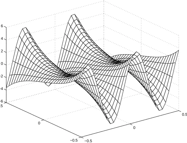
in a hollow domain (the region lying between a circleR = 1/2 and a square of 1/2×1/2 (Figure 2) with Dirichlet boundary conditions. The exact solution, which is plotted in (Figure 2), is given by
method is also considered here. It uses the same sets of interior points and inner boundary points as the proposed method. However, the outer boundary points are replaced with (Nx+Ny) points that are uniformly distributed along the circular boundary for a better performance. Since the DRBFN approximations are written in terms of network weights, it leads to the system matrix of dimension (Nip+Nbp)×(Nip+Nbp).
A number of uniformNx×Ny grids, namely 9×9,13×13,· · · ,101×101, are employed to study the convergence behaviour of the solution. Results concerning the condition number of the system matrix and the discrete relative L2 error of the interior solution are given
in Table 1. In terms of the condition number of the system, the proposed method yields condition numbers about four orders of magnitude lower than those associated with the conventional method. In terms of accuracy, more accurate results and faster convergence are achieved; for example, the convergence order and the L2 error (Ne at the finest grid
of 101×101) are O(h3.23) and 9.93×10⁻⁶ for the 1D-IRBFN method, and O(h1.52) and
2.02×10⁻³ for the DRBFN method. It can also be seen that the obtained convergence
rate O(h3.23) is faster than those of the standard Cartesian-grid methods reported in the
literature (aboutO(h2)). However, the present system matrix is not as sparse as those of
3
BIHARMONIC EQUATION WITH DIRICHLET
BOUNDARY CONDITIONS
3.1
Formulation
The process of deriving the 1D-IRBFN formulation for biharmonic equations is similar to that for Poisson equations. However, the corresponding equations involve more terms, and one needs to pay attention to the following two issues: (a) the implementation of double boundary conditions (u and ∂u/∂n) and (b) the treatment of mixed partial derivatives
∂4u/∂x2∂y2. Notations used in this section and in the previous one have similar meanings.
Consider a grid point x (Figure 1). The nodal points along the horizontal line pass-ing through point x are used to construct the approximations for u and ∂iu/∂xi (i =
{1,2,3,4})
∂4u(x)
∂x4 =
N
X
i=1
w(i)g(i)(x) =
N
X
i=1
w(i)H(i)
[4](x), (31)
∂3u(x)
∂x3 =
N
X
i=1
w(i)H[3](i)(x) +c1, (32)
∂2u(x)
∂x2 =
N
X
i=1
w(i)H[2](i)(x) +c1x+c2, (33)
∂u(x)
∂x = N
X
i=1
w(i)H[1](i)(x) +c1
x2
2 +c2x+c3, (34)
u(x) =
N
X
i=1
w(i)H[0](i)(x) +c1
x3
6 +c2
x2
Some relevant matrices and vectors to be used for the conversion process are given below H =
H[0](1)(x(1)) H(2)
[0] (x(1)) · · · H (N)
[0] (x(1)) x(1)3/6 x(1)2/2 x(1) 1
H[0](1)(x(2)) H(2) [0] (x
(2)) · · · H(N) [0] (x
(2)) x(2)3/6 x(2)2/2 x(2) 1
· · · ·
H[0](1)(x(N)) H(2)
[0](x(N)) · · · H (N)
[0] (x(N)) x(N)3/6 x(N)2/2 x(N) 1
b w= w(1) w(2) · · ·
w(N)
, bc=
c1 c2 c3 c4
, ub=
u(1) u(2) · · ·
u(N)
.
It can be seen that the presence of integration constants allows the addition of some extra equations to the conversion system. Given the double boundary conditions uand ∂u/∂n, it is straightforward to obtain the values of ∂u/∂x and ∂u/∂y along the boundaries. The additional matrix and vector can be generated as follows
K=
H
(1)
[1](x(1)) H (2)
[1] (x(1)) · · · H (N)
[1] (x(1)) x(1)2/2 x(1) 1 0
H[1](1)(x(N)) H(2) [1](x(
N)) · · · H(N) [1] (x(
N)) x(N)2/2 x(N) 1 0
, b f = ∂u ∂x(x
(1))
∂u ∂x(x
(N))
.
The conversion process thus becomes
bu
b f = H K wb
b
c
=C
wb
bc
, (36)
wb
b
c
=C−1
bu
b
f
Substitution of (37) into (31)-(34) yields
∂4u(x)
∂x4 =
H[4](1)(x), H[4](2)(x),· · · , H[4](N)(x),0,0,0,0C−1
bu
b
f
, (38)
∂3u(x)
∂x3 =
H[3](1)(x), H[3](2)(x),· · · , H[3](N)(x),1,0,0,0C−1
bu
b
f
, (39)
∂2u(x)
∂x2 =
H[2](1)(x), H[2](2)(x),· · · , H[2](N)(x), x,1,0,0C−1
bu
b
f
, (40)
∂u(x)
∂x =
H[1](1)(x), H[1](2)(x),· · ·, H[1](N)(x),x
2
2, x,1,0
C−1
bu
b
f
. (41)
Since u(1), u(N) and fbare known, the above expressions can be rewritten as
∂iu(x) ∂xi =D
IV
ix buip+k IV
ix , i={1,2,3,4}, (42)
where the superscript IV is used to indicate that Dix and kix are obtained using the
IRBF-4 scheme, DIV
ix are known matrices of dimension 1×(N −2), and kix are known
constants.
Similarly, the approximations for ∂iu/∂yi (i = {1,2,3,4}) at point x are constructed
using the nodal points along the vertical line passing through that point
∂iu(y) ∂yi =D
IV
iy buip+k IV
iy , i={1,2,3,4}. (43)
Applying (42) and (43) to the nodal points over the whole domain leads to
g
∂iu ∂xi =De
IV
ix euip+ekixIV, (44)
g
∂iu ∂yi =De
IV
iy euip+ek IV
where DeIV
ix and DeiyIV are known matrices of dimensions (Nip+Nbpx)× Nip and (Nip + Nbpy)×Nip, respectively.
The mixed fourth-order partial derivative ∂4u/∂x2∂y2 can be computed by means of
relevant second-order derivatives according to the following relation
∂4u ∂x2∂y2 =
1 2 ∂2 ∂x2
∂2u ∂y2 + ∂ 2 ∂y2
∂2u ∂x2
. (46)
Due to the fact that the cross derivative needs information from both x− and y− direc-tions, it is straightforward to obtain the values of this derivative only at the grid points (i.e interior points). Fortunately, the governing equation is required to be discretized at the interior points only. Expression (46) can be computed by
2 ∂g
4u
∂x2∂y2
!
ip
=De∗
2x
g
∂2u
∂y2
!
ip
+De∗
2y
g
∂2u
∂x2
!
ip
, (47)
where the construction of De∗
2x and De∗2y is similar to that of De2x (20) andDe2y (22), except
that the present training points do not include the boundary points (ek∗
2x = ek2∗y = []).
Substitution of (44) and (45) with i= 2 into (47) yields
2 ∂g
4u
∂x2∂y2
!
ip
=De∗
2x
e
D2IVy
ipuipe +
e
D∗
2y
e
D2IVx
ipeuip+
ek∗
4xy, (48)
=De∗
4xyuipe +ek4∗xy, (49)
where De∗
4xy is a known matrix of dimension Nip×Nip and ek4∗xy is a known vector.
Using (44), (45) with i = 4 and (49), the biharmonic equation ∇4u =b can be reduced
to the following square system of algebraic equations
g
∂4u
∂x4
!
ip
+ 2 g∂
4u
∂x2∂y2
!
ip
+ ∂g
4u
∂y4
!
ip
or
e
DIV
4x
ip+
e
D∗
4xy +
e
DIV
4y
ip
e
uip = (b)ip−ek4x
ip+
e
k∗
4xy +
e
k4y
ip
, (51)
or
e
Auipe =er, (52)
where Aeis an Nip×Nip matrix.
3.2
Numerical Results
The problem here is to find a functionu(x, y) satisfying the following biharmonic equation
∇4u= 256(π2−1)2[sin(4πx) cosh(4y)−cos(4πx) sinh(4y)] (53)
defined on an annulus domain of radii R1 = 1/4 and R2 = 1/2 (Figure 3) and subject to Dirichlet boundary conditions (u and ∂u/∂n). The exact solution (Figure 3) is given by
u= [sin(4πx) cosh(4y)−cos(4πx) sinh(4y)] (54)
from which the boundary data can be easily obtained.
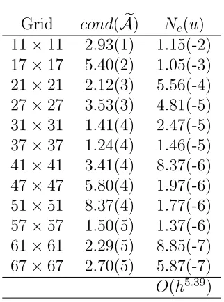
The convergence behaviour of the method is numerically investigated using a number of uniform Cartesian grids, 11×11,17×17,· · · ,67×67. Table 2 shows that the proposed method produces a very high convergence rate, O(h5.39). The condition numbers of the
system matrix are relatively low, only up to O(105). When compared to the case of
4
POISSON EQUATION WITH DIRICHLET AND
NEUMANN BOUNDARY CONDITIONS
4.1
Formulation
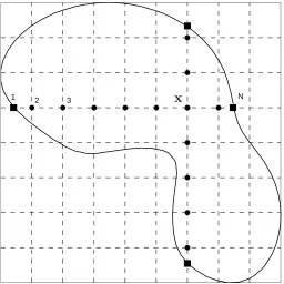
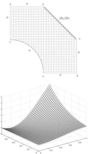
Special treatment is required for the imposition of Neumann boundary conditions at immersed boundaries. Viswanathan [26] proposed constructing a FD approximation at grid nodes that lie adjacent to the curved boundary by taking into account the rate of change of the normal gradient ofualong the boundary. In the work of Thuraisamy [6], the normal derivative at a boundary point was approximated using two lines that intersect at that point and make angles ofπ/4 on either side of the local normal direction. Recently, Sanmigue-Rojas et al [27] reported a technique for generating a non-uniform Cartesian grid in which all the boundary nodes are regular nodes of the grid. As a result, the values of derivatives with respect to x and y at the boundary points can be computed in a straightforward manner. The technique of Sanmigue-Rojas and his co-workers will be applied here to discretize sub-regions involving the Neumann boundary condition.
Consider a domain as shown in Figure 4. A Neumann boundary condition is specified on the segment CD, while Dirichlet boundary conditions are applied along AB, BC, DE, EF and FA (AB=BC=DE=EF=1/2). The requirement here is that the boundary points on the segment CD are also grid nodes, thereby avoiding the usual complicated interpolations at the boundaries. Let bp∗ denote the boundary points on CD. Since ip and bp∗ are grid nodes, one can easily obtain their 1D-IRBFN expressions for derivatives with respect tox
and y. To obtain the values ofuatipandbp∗, one needs to generate a set of (Nip+Nbp∗)
4.1.1 Approach 1
The system of equations is generated here by applying the governing equation to the interior points ip and by collocating the Neumann boundary condition at the boundary points bp∗.
The construction of the 1D-IRBFN approximations for this case is similar to the previous case of Poisson equation with Dirichlet boundary conditions. One only needs to pay a little attention to lines that cross the segment CD. For the vector buin (11)-(12), only the first component u(1) is given, while the remaining components {u(2), u(3),· · · , u(N)} are
unknowns to be found. Expressions (14) and (16) thus become
∂2u(x)
∂x2 =D2x
uipb
u(x(N))
+k2x, (55)
∂u(x)
∂x =D1x
uipb
u(x(N))
+k1x, (56)
u(x) = D0x
uipb
u(x(N))
+k1x, (57)
where kix (i={0,1,2}) are known constants whose values depend on u(1).
The assembly process leads to
g
∂2u
∂x2 =De2xeuip+bp∗+ek2x, (58)
f
∂u
∂x =De1xeuip+bp∗+ek1x, (59)
g
∂2u
∂y2 =De2yuipe +bp∗+ek2y, (60)
f
∂u
For this approach, the system of equations can be written as
g
∂2u
∂x2
!
ip
+ ∂g2u
∂y2
!
ip
=eb
ip (62)
nx ∂uf ∂x
!
bp∗
+ny ∂uf ∂y
!
bp∗
= ∂uf
∂n ! bp∗ , (63) or e
D2x
ip+
e
D2y
ip
e
uip+bp∗ =
eb
ip−
e
k2x
ip−
e
k2y
ip, (64)
nxDe1x
bp∗
+nyDe1y
bp∗
e
uip+bp∗ =
f
∂u ∂n
!
bp∗
−nxek1x
bp∗
−nyek1y
bp∗
, (65)
or
e
Auipe +bp∗ =er, (66)
wherenx and ny are the components of the unit vector normal to the boundary CD, and
e
A is an (Nip+Nbp∗)×(Nip+Nbp∗) matrix.
4.1.2 Approach 2
Unlike Approach 1, the nodal values of the Neumann boundary condition on the bound-ary CD are imposed through the conversion process. Consequently, it allows the exact satisfaction of the governing equation not only at the interior points ip but also at the boundary points bp∗.
the following equations
u(x(1)) =
N
X
i=1
w(i)H[0](i)(x(1)) +c1x(1)+c2, (67)
u(x(2)) =
N
X
i=1
w(i)H[0](i)(x(2)) +c1x(2)+c2, (68)
· · · ·
u(x(N)) =
N
X
i=1
w(i)H[0](i)(x(N)) +c1x(N)+c2, (69)
nx∂u ∂x(x
(N)) =
N
X
i=1
w(i)H(i) [1](x
(N)) +c
1, (70)
or in a matrix form
ub
nx∂u ∂x(x
(N))
=C
wb
b
c
, (71)
or
wb
b
c
=C−1
bu
nx∂u ∂x(x
(N))
=C−1
ub
∂u ∂n(x
(N))−ny∂u ∂y(x
(N))
. (72)
Since ∂u(x(N))/∂n is given and the value of ∂u(x(N))/∂y can be replaced with a linear
combination of nodal values of u using (61) (the expression of∂u/∂y from Approach 1), one can express the RBF coefficients in terms of nodal variable values. The remainder of the construction process is similar to those of the previous sections.
For this approach, the system of equations can be written as
g
∂2u
∂x2
!
ip+bp∗
+ ∂g
2u
∂y2
!
ip+bp∗
=eb ip+bp∗
, (73)
or
e
D2x
ip+bp∗
+De2y
ip+bp∗
e
uip+bp∗ =
eb
ip+bp∗
−ek2x
ip+bp∗
−ek2y
ip+bp∗
or
e
Auipe +bp∗ =er, (75)
where Aeis an (Nip+Nbp∗)×(Nip+Nbp∗) matrix.
4.2
Numerical Results
The proposed method is applied to solve the Poisson equation of the form
∇2u= 4 [cos(2x) cosh(2y) + sin(2x) sinh(2y)] (76)
with the exact solution being
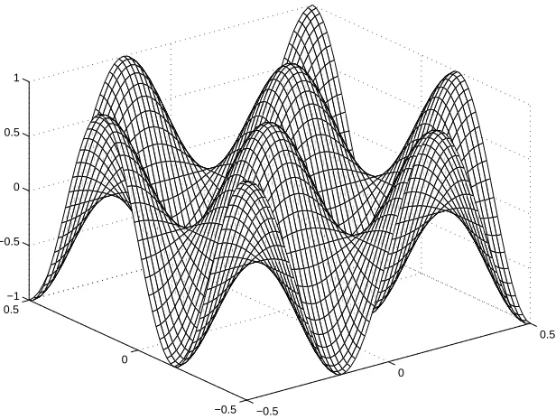
u=x[sin(2x) cosh(2y)−cos(2x) sinh(2y)]. (77)
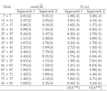
The variation of (77) over the square that covers the problem domain is plotted in Figure 4. A number of uniform grids, 7×7,11×11,· · · ,81×81, are employed. Table 3 reveals that Approach 2 is superior to Approach 1 with respect to the condition number of the system matrix, accuracy and convergence rate. The proposed method converges apparently as
O(h1.93) for Approach 1 andO(h2.40) for Approach 2. At the finest grid,Nes are 6.88×10⁻⁵
and 3.34×10⁻⁶ for Approach 1 and Approach 2, respectively. Imposing normal derivatives
by means of integration constants is recommended for use.
5
CONCLUDING REMARKS
interpolation scheme. Three types of problems, namely Poisson equation with Dirich-let boundary condition, biharmonic equation with DirichDirich-let boundary condition, Poisson equation with Dirichlet and Neumann boundary conditions, are investigated. The nodal values of the variable along the boundary can be accommodated straightforwardly, while the boundary values of its normal derivative can be imposed effectively through the pro-cess of converting network weights into nodal variable values. The proposed method requires much less computational effort than the 2D-IRBFN method. Numerical tests show that the method yields fast convergence, i.e third- and fifth-order accuracy with respect to grid size for the the solution of second- and fourth-order PDEs, respectively.
ACKNOWLEDGEMENTS
This research was supported by the Australian Research Council. Dr. N. Mai-Duy is the recipient of an Australian Research Council Post-Doctoral Fellowship. The authors would like to thank the referees for their helpful comments.
REFERENCES
1. T. Belytschko, Y. Krongauz, D. Organ, M. Fleming and P. Krysl, “Meshless meth-ods: an overview and recent developments,” Computer Methods in Applied Me-chanics and Engineering, 139, 3 (1996).
2. S.N. Atluri and S. Shen, The Meshless Local Petrov-Galerkin Method, Tech Science Press, Encino, 2002.
3. S. Li and W.K. Liu, “Meshfree and particle methods and their applications,” Applied Mechanics Reviews, 55(1), 1 (2002).
5. V. Thuraisamy, “Approximate solutions for mixed boundary value problems by finite-difference methods,” Mathematics of Computation, 23(106), 373 (1969). 6. V. Thuraisamy, “Monotone type discrete analogue for the mixed boundary value
problem,” Mathematics of Computation, 23(106), 387 (1969).
7. H. Johansen and P. Colella, “A Cartesian grid embedded boundary method for Poisson’s equation on irregular domains,” Journal of Computational Physics, 147(1), 60 (1998).
8. T. Ye, R. Mittal, H.S. Udaykumar and W. Shyy, “An accurate cartesian grid method for viscous incompressible flows with complex immersed boundaries,” Journal of Computational Physics, 156(2), 209 (1999).
9. F. Gibou, R.P. Fedkiw, L.-T. Cheng and M. Kang, “A second-order-accurate sym-metric discretization of the Poisson equation on irregular domains,” Journal of Com-putational Physics, 176(1), 205 (2002).
10. Z. Jomaa and C. Macaskill, “The embedded finite difference method for the Poisson equation in a domain with an irregular boundary and Dirichlet boundary condi-tions,” Journal of Computational Physics, 202(2), 488 (2005).
11. S. Haykin, Neural Networks: A Comprehensive Foundation, Prentice-Hall, New Jersey, 1999.
12. W.R. Madych and S.A. Nelson, “Multivariate interpolation and conditionally posi-tive definite functions,” Approximation Theory and its Applications, 4, 77 (1988). 13. W.R. Madych and S.A. Nelson, “Multivariate interpolation and conditionally
posi-tive definite functions, II,” Mathematics of Computation, 54(189), 211 (1990). 14. E.J. Kansa, “Multiquadrics- A scattered data approximation scheme with
elliptic partial differential equations,” Computers and Mathematics with Applica-tions, 19(8/9), 147 (1990).
15. G.E. Fasshauer, “Solving partial differential equations by collocation with radial basis functions,” in Surface Fitting and Multiresolution Methods, A. LeMhaut, C. Rabut and L.L. Schumaker (Editors), Vanderbilt University Press, Nashville, TN, 1997, p. 131.
16. M. Zerroukat, H. Power and C.S. Chen, “A numerical method for heat transfer problems using collocation and radial basis functions,” International Journal for Numerical Methods in Engineering, 42, 1263 (1998).
17. E.J. Kansa and Y.C. Hon, “Circumventing the ill-conditioning problem with multi-quadric radial basis functions: applications to elliptic partial differential equations,” Computers and Mathematics with Applications, 39, 123 (2000).
18. N. Mai-Duy and T. Tran-Cong, “Numerical solution of differential equations using multiquadric radial basis function networks,” Neural Networks, 14(2), 185 (2001). 19. C. Shu, H. Ding and K.S. Yeo, “Local radial basis function-based differential
quadra-ture method and its application to solve two-dimensional incompressible Navier-Stokes equations,” Computer Methods in Applied Mechanics and Engineering, 192, 941 (2003).
20. N. Mai-Duy and T. Tran-Cong, “Approximation of function and its derivatives using radial basis function networks,” Applied Mathematical Modelling, 27, 197 (2003). 21. N. Mai-Duy, “Indirect RBFN method with scattered points for numerical solution
of PDEs,” Computer Modeling in Engineering and Sciences, 6(2), 209 (2004). 22. N. Mai-Duy and R.I. Tanner, “Solving high order partial differential equations with
23. N. Mai-Duy and T. Tran-Cong, “An efficient indirect RBFN-based method for nu-merical solution of PDEs,” Nunu-merical Methods for Partial Differential Equations, 21, 770 (2005).
24. N. Mai-Duy and T. Tran-Cong, “Solving biharmonic problems with scattered-point discretisation using indirect radial-basis-function networks,” Engineering Analysis with Boundary Elements, 30(2), 77 (2006).
25. P.J. Roache, Computational Fluid Dynamics, Hermosa Publishers, Albuquerque, 1980.
26. R.V. Viswanathan, “Solution of Poisson’s equation by relaxation method–normal gradient specified on curved boundaries,” Mathematical Tables and Other Aids to Computation, 11(58), 67 (1957).
Table 1: Example 1 (Poisson equation, Dirichlet boundary conditions): Condition number and accuracy obtained by the conventional DRBFN and the proposed 1D-IRBF methods. Notice that h is the spacing (grid size) and a(−b) means a×10−b.
Grid cond(Ae) Ne(u)
DRBFN 1D-IRBFN DRBFN 1D-IRBFN 9×9 1.67(4) 3.81(0) 1.27(-1) 1.08(-1) 13×13 6.96(4) 1.98(1) 4.24(-2) 8.30(-3) 17×17 1.68(5) 3.52(1) 3.14(-2) 1.78(-3) 21×21 3.34(5) 6.03(1) 2.56(-2) 1.06(-3) 25×25 5.88(5) 4.55(1) 1.71(-2) 5.57(-4) 29×29 9.39(5) 6.19(1) 1.25(-2) 4.26(-4) 33×33 1.44(6) 1.31(2) 9.26(-3) 2.46(-4) 37×37 2.05(6) 1.62(2) 7.72(-3) 1.91(-4) 41×41 2.83(6) 2.62(2) 6.96(-3) 1.39(-4) 45×45 3.76(6) 2.59(2) 7.57(-3) 1.11(-4) 49×49 4.94(6) 3.77(2) 5.94(-3) 8.27(-5) 53×53 6.26(6) 3.37(2) 4.86(-3) 6.71(-5) 57×57 7.88(6) 4.90(2) 4.29(-3) 5.27(-5) 61×61 9.69(6) 5.24(2) 3.91(-3) 4.36(-5) 65×65 1.17(7) 5.94(2) 4.16(-3) 3.71(-5) 69×69 1.41(7) 6.84(2) 3.87(-3) 3.13(-5) 73×73 1.67(7) 8.00(2) 3.32(-3) 2.59(-5) 77×77 1.97(7) 8.13(2) 2.91(-3) 2.21(-5) 81×81 2.30(7) 9.21(2) 2.68(-3) 1.89(-5) 85×85 2.66(7) 1.31(3) 2.51(-3) 1.64(-5) 89×89 3.06(7) 1.39(3) 2.48(-3) 1.45(-5) 93×93 3.50(7) 1.03(3) 2.45(-3) 1.30(-5) 97×97 3.98(7) 1.45(3) 2.22(-3) 1.12(-5) 101×101 4.50(7) 1.34(3) 2.02(-3) 9.93(-6)
Table 2: Example 2 (biharmonic equation, Dirichlet boundary conditions): Condition number and accuracy. Notice that his the spacing (grid size) and a(−b) means a×10−b.
Grid cond(Ae) Ne(u) 11×11 2.93(1) 1.15(-2) 17×17 5.40(2) 1.05(-3) 21×21 2.12(3) 5.56(-4) 27×27 3.53(3) 4.81(-5) 31×31 1.41(4) 2.47(-5) 37×37 1.24(4) 1.46(-5) 41×41 3.41(4) 8.37(-6) 47×47 5.80(4) 1.97(-6) 51×51 8.37(4) 1.77(-6) 57×57 1.50(5) 1.37(-6) 61×61 2.29(5) 8.85(-7) 67×67 2.70(5) 5.87(-7)
Table 3: Example 3 (Poisson equation, Dirichlet and Neumann boundary conditions): Condition number and accuracy obtained by the proposed method. The Neumann bound-ary conditions are imposed by adding addition equations to the system for Approach 1, and by means of integration constants for Approach 2. Notice that h is the spacing (grid size) and a(−b) meansa×10−b.
Grid cond(Af) Ne(u)
Approach 1 Approach 2 Approach 1 Approach 2 7×7 2.01(2) 9.21(1) 1.00(-2) 2.20(-3) 11×11 5.47(2) 3.35(2) 3.91(-3) 4.13(-4) 17×17 2.06(3) 9.18(2) 1.62(-3) 1.17(-4) 21×21 3.99(3) 1.45(3) 1.05(-3) 6.85(-5) 27×27 9.34(3) 2.47(3) 6.33(-4) 3.70(-5) 31×31 1.51(4) 3.30(3) 4.79(-4) 2.69(-5) 37×37 1.67(4) 4.76(3) 3.34(-4) 1.79(-5) 41×41 2.25(4) 5.89(3) 2.72(-4) 1.42(-5) 47×47 3.40(4) 7.79(3) 2.06(-4) 1.05(-5) 51×51 4.43(4) 9.21(3) 1.75(-4) 8.84(-6) 57×57 6.85(4) 1.15(4) 1.39(-4) 7.01(-6) 61×61 7.95(4) 1.32(4) 1.21(-4) 6.04(-6) 67×67 1.08(5) 1.60(4) 1.00(-4) 4.96(-6) 71×71 1.32(5) 1.80(4) 8.98(-5) 4.40(-6) 77×77 1.48(5) 2.12(4) 7.62(-5) 3.71(-6) 81×81 1.68(5) 2.35(4) 6.88(-5) 3.34(-6)
1 2 3 x N
−0.5
0
0.5
−0.5 0
[image:30.612.158.466.361.593.2]0.5 −1 −0.5 0 0.5 1
−0.5
0
0.5
−0.5 0
[image:31.612.161.465.368.600.2]0.5 −6 −4 −2 0 2 4 6
A B C D
E
F
u
u
u
u u
∂u/∂n
0
0.2 0.4
0.6 0.8
1
[image:32.612.163.462.76.598.2]0 0.2 0.4 0.6 0.8 1 −1 0 1 2 3 4 5