This is a repository copy of Distributional logic programming for Bayesian knowledge
representation.
White Rose Research Online URL for this paper:
http://eprints.whiterose.ac.uk/108706/
Version: Accepted Version
Article:
Angelopoulos, Nikolaos and Cussens, James orcid.org/0000-0002-1363-2336 (2016)
Distributional logic programming for Bayesian knowledge representation. International
Journal of Approximate Reasoning. pp. 52-66. ISSN 0888-613X
https://doi.org/10.1016/j.ijar.2016.08.004
[email protected] Reuse
Items deposited in White Rose Research Online are protected by copyright, with all rights reserved unless indicated otherwise. They may be downloaded and/or printed for private study, or other acts as permitted by national copyright laws. The publisher or other rights holders may allow further reproduction and re-use of the full text version. This is indicated by the licence information on the White Rose Research Online record for the item.
Takedown
If you consider content in White Rose Research Online to be in breach of UK law, please notify us by
Distributional Logic Programming for Bayesian
Knowledge Representation
Nicos Angelopoulosc, James Cussensd
aWelcome Trust Sanger Institute, Hinxton, CB10 1SA, UK bDepartment of Computer Science,University of York, York UK
Distributional Logic Programming for Bayesian
Knowledge Representation
Nicos Angelopoulosc, James Cussensd
cWelcome Trust Sanger Institute, Hinxton, CB10 1SA, UK dDepartment of Computer Science,University of York, York UK
1. Introduction
Bayesianism provides a powerful framework for reasoning with statistical knowl-edge. The result of reasoning is captured by the posterior distribution. Knowledge is captured by the prior and the evidence. The former can represent expert knowledge or belief in a domain, while the latter can take the form of data to be analysed. The basic Bayesian premise can be summarised as:
posterior ∝ prior × evidence
A plethora of algorithms operate on the above principle to either locate important mem-bers of the posterior, such as the maximum a posteriori mode (MAP), or to characterise the whole distribution. Computation in both cases is often prohibitively lengthy to allow exact algorithms, so approximations are routinely used. These include varia-tional methods [26] which approximate the inference on the evidence by considering a simpler inference task while Markov chain Monte Carlo (MCMC) simulations approx-imate the whole posterior by means of a stochastic search.
Bayesian algorithms that take into account the prior part of the above premise often do so in a restricted form. For instance, [10] uses a conjugate prior over classification trees and in [21] the authors use an uninformative prior over BNs. Reasons for such restrictions include both the lack of relevant knowledge and the limited availability of formalisms that can express the known biases and for which effective inference procedures exist. However, in application areas such as computational biology and bioinformatics a growing amount of formalised knowledge is becoming available. The ability to represent complex biological knowledge would greatly benefit the application of Bayesian methods in these areas as it can focus computational resources in parts of the solution space that are most likely to hold the answer or of particular interest to the biologists. On the other hand, Bayesian methods provide a convenient, clean framework in which such knowledge can be incorporated.
and the Kyoto Encyclopedia of Genes and Genomes (KEGG, [27]) are gaining ground in both depth and breadth of the knowledge they store.
Logic programming (LP) is an attractive formalism for representing crisp knowl-edge. Probabilistic extensions to logic programming have been previously proposed for the purpose of representing Bayesian priors ([13, 3, 6]). Here, we present an ex-pressive language that extends logic clauses with probabilities which are calculated by guards encoding arbitrary relations. We also provide a characterisation that eluci-dates the interplay of nondeterminism in LP and probabilistic reasoning for a number of generative languages. Additionally, we put emphasis on representing knowledge for effective probabilistic problem solving via a number of examples that represent knowledge over model structures and which are drawn from the literature. We de-tail how the probabilistic aspects of our formalism enable Bayesian learning that can exploit both the prior information and the internal probabilistic choice points to cre-ate a search space constrained Metropolis-Hasting algorithm. This paper provides the knowledge representation machinery for the conceptual framework of [3] and the ma-chine learning results of [4, 5, 6, 7]. The full syntax is presented for the first time, along with semantic considerations and a thorough discussion and mathematical framework for probabilistic paths (Section 4). Furthermore, details on constructing effective priors that model priors from the literature are discussed. Finally, we illustrate how the knowl-edge representation discussed in this paper connects to already published research that concentrated on machine learning results [4, 5, 6, 7].
2. Preliminaries
In this section we review the necessary terminology from logic programming. A logic programLis a set of clauses of the form Head :- Body defining a number of predicates. Headis an atom, a single positive literal constructed from a predicate symbol and a number of term arguments.Bodyis a conjunction of zero or more atoms
A1, . . . An. Each term is a recursively defined structure that might be an atomic value, a
variable or a function constructed by an atomic function symbol andnterm arguments. The formHead:-Bodyis syntactic sugar for the disjunctionHead∨¬A1∨· · ·∨¬An
with all variables implicitly universally quantified. We follow LP conventions and have variables starting by a capital letter (List) and atoms by a lower case letter (constant). An example term of 4 arguments is: cart(f1, v1, L, R). It represents a classification tree which splits some data at the top level on featuref1and valuev1, while the left (L) and right (R) branches are as yet to be constructed and are shown here as free variables.
A query or goalG1is a disjunction of negative literals(¬A(1,1)∨. . .∨ ¬A(1,n)) which the logic engine attempts to refute using the clauses inL. This is done by em-ploying SLD (linear resolution of definite clauses with a selection rule). Linear resolu-tion at stepiwill resolve¬A(i,1)with the head (Hi) of the first matching clause found
(Mi) and replace it with the body of the clause thus generating a new goal. Matching
is via the unification algorithm, which when successful, provides a substitutionθisuch
thatA(i,1)/θi = Hi/θi. Intuitively, successful unification is a method for selecting
which of the clauses in the program are applicable in answering the query whileθi
to the query. A computation terminates when the current goal is the empty one or no matching clause is found. In the former case an overall substitution is constructed
θ= (θN, . . . , θ1)whereθis the composition of the substitutionsθN, . . . , θ1withG/θ
being the computed answer.
The logic engine explores yet unexplored parts of the space, by returning to the latest matching step and attempting to find alternative resolution clauses. In logic pro-gramming parlance, this is a backtracking step. In the case where no matching clauses are found, the engine will backtrack to the the second latest matching step, and thus recursively search until an alternative can be found. Computed answers in the form ofθxsubstitutions done after the backtracking point are undone. The complete search
ends when all alternatives have been exhausted. In what follows we will useAito refer
toA(i,1), that is, the literal used for theith resolution step.
As an illustrating example program, consider the following two clauses defining
themember/2predicate:
member(H,[H|T]). (C1)
member(El,[H|T]) :− (C2)
member(El, T).
The first clause, (C1), states that the head of a list is its first element, while the second clause states that element El is a member of the list, if it is a member of the tail (T) of the list. Lists are convenient recursive term structures commonly used in logic programming to hold a collection of data objects. Posed with a query of the form
?−member(X,[a, b, c])(which is syntactic sugar for¬member(X,[a, b, c])) the logic
programming engine uses SLD resolution which scans the query left to right and the program top to bottom as to provide all possible answers in the form of values forX. In our example these are the alternative valuesa,b, andcwhich are formally written asθ={X=a},θ={X =b}andθ={X =c}.
2.1. Probability Theory and Logic Programming
Logic programming implements a complete search of a nondeterministic space. We review the difficulties of mixing such spaces with probabilistic ones and present one way to achieve this. The formalism we propose here assigns probabilities to clauses defining a single probabilistic space based on a clear distribution over computed an-swersG/θ. Furthermore, the thesis we propose is that for a class of generative logic programming formalisms that treat probabilities as top-level constructs the definition of a single probabilistic space with a clear distribution over computed answersG/θis a key concept.
probabilistic construct that instantiates an unbound variable from the elements of a list according to the probability values attached to each element. Dlp is closely related to PRISM and to SLPs; we will explain the similarities and differences in Section 4.1. Another language is ProbLog [28]. This generalises the concept of assigning probabil-ities to a list of values by removing the requirement for independence between random variables.
PCLP [33] and clp(pfd(Y)) [1] employ constraint programming to create, in dis-tinct ways, two separate spaces. Nondeterminism is expressed via clausal syntax while the probabilistic is constructed in the constraint store with the constraint solver used to reason/infer from this information. A crucial point in understanding the differences of nondeterminism to probabilistic reasoning as discussed here, is that of a single substi-tution (θ) appearing twice. In terms of standard logic programming, the repetition of an already seen solution is immaterial, as the second appearance adds nothing new in terms of logical consequence with the possible exception of explanation-based interpre-tations. On the other hand, multiple probabilistic derivations of the same consequences are intrinsically important as they alter the probability attached to eachθ.
2.2. Statistical relational learning
Related research areas include that of statistical relational learning with important recent contributions such as: probabilistic relational models (PRMs, [20]), Markov logic networks (MLNs, [19]) and ProPPR [39]. These approaches use relations and logic for representing knowledge. Inference is layered on top by the statistical ma-chinery. ProPPR has been presented as an extension to SLPs which locally grounded and was introduced with the specific aim of a efficient alternative for implementing the personalised PageRank algorithm [11]. In comparison, distributional logic pro-gramming (Dlp) focuses on logic propro-gramming as a general purpose AI language by extending logical reasoning with probabilistic knowledge. The statistical machinery is built in confluence with the underlying logic inference. Figaro [30] is a powerful object oriented probabilistic programming language also coupled to a Metropolis-Hastings (MH). It is more general in that it allows objects to have constraints and relationships to other objects. In contrast, Dlp is based on logic programming which makes programs readily amenable to mathematical analysis and program transformations.
It is worth noting that probabilistic programming has seen an increase in research interest, with a number of formalisms from other paradigms. Two such systems are Church [23] and Anglican [41] that extend functional programming with probabilistic constructs.
3. Syntax
Definition 1. Let H :−B be a syntactically correct Prolog clause andφ(H) =
f unctor(H)/arity(H) be the structure denoting the functor and arity of H. Let
VGφ(H) be a list of variables andEGφ(H) an arithmetic expression involving the
vari-ables inVGφ(H) and no other variables. A probabilistic predicatePφ(H)is associated
with a single guardGφ(H)and consists of clauses of the form:
EGφ(H) ::VGφ(H) ::H :-B (C3)
We will refer toEGφ(H)as the probabilistic expression of the clause and toVGφ(H)
as the probability measure variables or simply measure variables of the clause. The probabilistic expression of a specific clause will be evaluated at resolution time to a number: the probability label of the resolved clause. The evaluation is preceded by the matching ofVGφ(H)to a list of ground arithmetic values generated by the guardGφ(H)
associated withPφ(H). Note that all clauses belonging to the same predicate should
share equal length probability measure variable lists (VGφ(H)), as they will be matched
to a list of numbers generated by a single guard. The computation of the associated guardGφ(H)occurs deterministically and if it fails or if it does not instantiateVGφ(H)
to a list of numbers, the computation halts.
Definition 2. LetAφ(H) be a goal,VAφ(H) a list of variables inAφ(H)andPφ(H) a
probabilistic predicate as defined in Definition 1. LetHǫ be a form ofP
φ(H)’s head
(H) with all its arguments replaced by variables andΛHǫ be a list of some of these variables. The single guardGφ(H)associated withPφ(H)is defined by:
VAφ(H) ::Aφ(H)∼ΛHǫ::H
ǫ (G1)
The list of variablesVAφ(H)constitutes the measure variables of the guard, and its
length should match the length of the measure variables list in the clauses ofPφ(H),
VGφ(H) in (C3), as they will be matched to them at run-time. H
ǫwill typically share
variables withAφ(H). These shared variables are the measure defining variables of the
guard, and are distinct to those inΛHǫ, which are the distributional or probabilistic
variables of the guard and associated predicate. Having a single guard means that the probabilistic dependencies of the data objects present as arguments to a predicate definition, can be defined in one place, capturing the probabilistic relation of the data and allowing the distillation onto the measure variables which in turn are used in the evaluation of the run-time probability expressions.
The intuitive reading of the measure variables inVAφ(H) of (G1) is that the
proba-bility by which data corresponding to theΛHǫ variables (by extensionPφ(H)too) are
generated, depends on the data in the shared variables ofHǫandA
φ(H). The
magni-tude of the dependency is defined byAφ(H)- an arbitrary logic goal, called at run-time.
Aφ(H) should be a pure logic goal, with no internal calls to probabilistic predicates. Communicating the results from the guard to the clauses is done via matching the po-sitioning of the variables inVGφ(H) to those ofVAφ(H). Concrete probabilistic labels
For example the following guard:
[L] ::length(List, L)∼[El] ::umember(El, List) (G2)
declares that the length L of the predicate’sumember/2input listListis the numeri-cal information needed to define a distribution over selecting an element from the input. Furthermore, in the case whereVAφ(H) andΛHǫare lists of one element we simplify
the notation by dropping the surrounding square brackets and writing (G2) as
L::length(List, L)∼El::umember(El, List) (G3)
The complete program corresponding to theumember/2example guard shown in (G2) is:
L::length(List, L)∼El::umember(El, List)
1
L ::L::umember(El,[El|T ail]). (C4)
1− 1
L ::L::umember(El,[H|T ail]) :− (C5)
umember(El, T ail).
The above program defines a uniform distribution over element selection for an input list irrespective of the length of this list. However, its execution according to what described so far, is computationally wasteful when consecutively calling the guard for
umember/2(Gumember/2) via the recursive call of (C5). For each application of the
recursive clause (C5) the length of the remaining list needs to be recalculated as to provide the measure variables ofumember/2. In order to address this inefficiency we introduce new syntax in the form of probabilistic goals.
Definition 3. LetF be a standard logic goal, H:−Ba logic clauseCor the logic part of a probabilistic clause, withB a conjunction of atomsA1, . . . , An(Section 2).
LetVC be a list combining variables inC and numeric values, with its length being
equal toVAφ(F)(Defn. 2). ForAicalling the probabilistic predicatePφ(F), we refer to
Aias a probabilistic goal if and only if it is of the form
VC::F (G4)
VCare the measure variables of the goal. The intuition behind probabilistic goals
is that when callingFin the context ofC, we might already have the necessary infor-mation regarding the relevant guard’s measure variables. So there will be no need to re-evaluateGφ(F). A typical category of predicates for which this is the case, is that of
and as before, ifVC is not instantiated to a list of arithmetic values the computation
stops. In terms of correctness, one could have a special execution mode which ensures that for a given query the values inVC of a probabilistic goal as shown in (G4) are
equal to those calculated by the guard inVGφ(A)of Definition 2.
The example program can now be written as:
L::length(List, L)∼El::umember(El, List) (G5)
1
L ::L::umember(El,[El|T ail]). (C6)
1− 1
L ::L::umember(El,[H|T ail]) :− (C7)
K is L−1,
K::umember(El, T ail).
The probabilistic expressions of clauses (C6,C7) will be computed at resolution time. Clause (C6) is labelled by L1 whereLis the length of the input list (as defined by stan-dard predicatelength/2).Lis computed at run-time by calling?−length(List, L)
which when called with a free variableLand a list of valuesListinstantiatesL to the length of the list. Clause (C7) claims the residual probability (1− L1). The re-cursive call has a label which carries forward the length ofT ail, the tail of the in-put list. This is one less than that of list [H|T ail]. By adding K as the label to the goalK :: umember(El, T ail), we avoid recomputing the guard. For the query
?−umember(X, List)whereListis a known list, the above program defines a
uni-form distribution over all the possible element selections from this list. The probabili-ties for the three possible selections (substitutions) for query
?−umember(X,[a, b, c]). (Q1)
are all equal to13and are computed by13,23×12, and23×12×1forX =a, X=band
X=c respectively.
A distributional logic programRis the union of a set of definite clausesLand a set of probabilistic clausesD. Both sets define the logical semantics ofRin unison while
Dalso defines a distribution over the substitution of the logical queries posed against
R.
4. Probabilistic paths
Recall the description of SLD-resolution given in Section 2. For query goalAlet
Aibe the selected goal for resolution at stepiandMia matching probabilistic clause.
We defineIthe index ofMi inR, such thatMi =RI (whereRI is theIthclause in
R).Eithe probabilistic expression ofMi,Githe guard ofMi(Giis short forGφ(Mi)
as defined in Defn. 1) andθ′
Gito be a complete substitution that grounds all the input
the logical parts ofR and eval(E) a function that evaluates arithmetic expressionE. The refutation choiceπi, that is the selection of which clause was used for theithstep
can be captured by
πi=
(I, eval(Ei/θU′i)) ifMi∈D∧R⊢Ui/θ
′ Ui
I ifMi∈L
The intuition is that a choice point can be abstracted to the identity of the clause used and the value of the label (probability) at run-time. Each refutation that involves a probabilistic clause produces answers of the formA/θπwhereπ= (π1, . . . , πN)is the
path of the refutation along with the probabilities attached to each choice. Similarly for iterationiwe defineπ(Ai) = (π1, . . . , πi−1), the partial path to that point. The procedure described above does not specify which literal¬A in the current goal is chosen for the next resolution step as our analysis is independent of this choice.
For queryAwe defineΛAto be the set of probabilistic variables inA.V ∈ΛAif and only if it is a variable inAand it will be matched during refutation to the output variables of a guard (V ∈ΛHǫas per Defn. 1). We restrict the class of allowable
com-binations of programs and queries (A) so that eachV can only be further instantiated by unifications to the same predicate. In theumember/2example (G5,C6,C7) and for query?−umember(X,[a, b, c]),X is a probabilistic variable and it only gets instan-tiated by the first argument ofumember/2which belongs toΛumember/2(see, (G5) and Defn. 2). Similarly, the probabilistic variables of a clause are those identified by the predicate guard, thus,Λφ(Mi)are the probabilistic variables ofMi.
We defineπ∼(Ai) as the list of choice points (clause indices) in the path that have
so far involved unification of the probabilistic variables ofMi. For example at the
end of deriving?−umember(X,[a, b, c]).forX =cagainst the program in clauses (G5,C6,C7), we haveπ∼(member(X,[a, b, c])X
=c) ={C7,C7,C6}, that is the prob-abilistic variable was passed through twice the recursive clause (C7) and once through the base, terminating, clause (C6). In this example, π(member(X,[a, b, c])X=c) =
{(C7,2/3),(C7,1/2),(C6,1)}. In general,π∼(Ai) is a subset of the choice points that
appear inπ(Ai). Choice points that are inπ(·)but notπ∼(·) are either missing due to
probabilistic goals that do not involve the probabilistic variables in the query, or due to refutations of non-probabilistic goals.
More formally,π∼(Ai) = (J·(J, X
j)∈π(Ai)∧T ∈Λφ(Mj)∧V ∈ΛAj∧V /θj ≺
T), whereV /θj≺Tis true if and only ifθjis a non empty substitution andV /θj =T.
That is,V is not a variable renaming equivalent term toT. Recall thatθjis thejstep
unification substitution withinπ(Ai). Functionuniq(θ, π, i)is defined to be true if and only ifπ∼(Ai) is unique for each distinctA/{θ
1, θ2, . . . , θi−1}. Letπ⊳(Ai)be
the sum of probabilities for clauses that lead to at least one refutation when they are resolved againstAigiven that the choices leading toAiare (π1, . . . , πi−1).
Definition 4. For programR, goalAand substitutionθwe define the following prob-ability distribution:
PR(A/θ) = X
π·R⊢A/θπ
Y
i·uniq(θ,π,i)
eval(Ei)
π⊳(Ai) (1)
uniq(·)have well-defined distributions. The constraint states that eachA/{θ1, θ2, . . . ,
θn−1}should correspond to a unique probabilistic pathπ∼(Ai) thus ensuring that a well-defined probabilistic space is considered.
The denominator in (1) normalises each choice ensuring thatP
θPR(G/θ) = 1.
In the naive case calculatingπ⊳(Ai)is a prohibitively expensive operation, as at least
one derivation for each possible continuation needs to be found. However, there are two interesting special cases. The first is whenRcan be shown to have no probability mass loss in which caseπ⊳(Ai) = 1 ⇒ P
θ∈ΘP(G/θ) = 1and the second when
all unifiable clauses forAi(u(Ai)) lead to at least oneθ, thenπ⊳(Ai)is replaced by P
a∈u(Ai)eval(Ea). Both properties may hold even in the case of infinite iand are
static properties of a program with regard to a class of queries. The main intuition behind Definition 4 is that the narrowing or instantiation of probabilistic variables inG
can be traced via the probabilistic variables in clauses used in resolution. Unification operations involving these variables are of particular interest as they define a single probabilistic space. Programs and associated queries for which nondeterministic and probabilistic predicates that incur no direct manipulation to the query probabilistic vari-ables produce a singleπ∼(Ai)for each probabilisticA
idefine a unique probabilistic
space that provides a sound platform for doing inference. This is certainly the case in the context of the inference we describe later in this paper, but likely to also hold for other types of probabilistic inference. In terms of the relation betweenπ(·)andπ∼(·)
these well behaved programs are characterised by the fact that there is an one-to-one mapping betweenπ(·)andπ∼(˙). This is a property of the program, and not a test of
admissibility for the inference described herein. We will term such programs and as-sociated queries as exhibiting”probabilistic determinism”. In general,π∼(·)provides
an abstract operational means for describing probabilistic aspects of probabilistic logic programs.
4.1. Paths in generative languages
The distribution we defined over substitutions has similarities with both the distri-butions over observables by [18] in PCCP and yields by [15] in pure normalised SLPs. However, both these formalisms steer clear of mixing probabilistic reasoning and non-determinism. PCCP replaces the nondeterministic operator of CCP by a probabilistic one and thus it does not allow any nondeterminism. This corresponds to programs where non probabilistic predicates are defined by single clauses. Clearly the unique-ness constraint is satisfied in this case. Furthermore, as PCCP is not concerned with failures, the sum of matchingeval(Ei)can be used instead ofπ⊳(Ai).
A stochastic clause in SLPs is a clause labelled by a number. [13] presented log-linear semantics for pure normalised SLPs. This is a program that only contains la-belled clauses. Following standard statistical practice, their semantics normalise over the partition function (Z), which for an SLP is equal to the sum of probabilities over
∪θ. A pure normalised SLP corresponds to a Dlp program that has just numbers as ex-pressions, guards are the true goal having no guard variables and all head variables in a clause are considered probabilistic. When there is no probability mass loss in theCi
normalised SLP can be mapped to a valid Dlp program. However, the opposite is not true. For instance, there is no intuitive way to code theumember/2program defined by clauses (C6-C7). The semantic arguments we have put forward in this paper can be viewed as an operational extension to the semantics given by Cussens [15]. Probabilis-tic paths provide a constructive history of the proof that can be used to pinpoint classes of programs and queries with desirable properties. In particular, we have argued that the desirable behaviour of pure, normalised SLPs can be seen as one manifestation of the general property ofprobabilistic determinism.
The logical-statistical programming language PRISM [35] provides a single primi-tive,msw/3, which implements aswitch: a selection of an element from a list accord-ing to an explicit fixed distribution over the list elements. This primitive is a fact, that is a clause with an empty body. In order for a query to have correct distributional seman-tics, eachθshould have a one-to-one correspondence with possible switch outcomes. PRISM presents an appealing primitive abstract machine for mixing logic program-ming and probabilistic reasoning. It has been used in efficient parameter estimation [34].
SLPs, PRISM and the much earlier formalism theIndependent Choice Logic (ICL)
[31, 32] have been shown to be very closely related. In each case a simple ‘base’ joint probability distribution is defined as a product of independent random variables. This is then extended to a more complex probability distribution using a logic program. In SLPs, the base distribution is over the choice of clause. In PRISM the base distribution is defined by theswitches. In ICL the base distribution is defined usingalternatives: sets of logical atoms exactly one of which can be true. Details can be found in [16].
Dlp extends this approach in one crucial way: the probabilities defining the ‘base’ distribution are notfixed. In contrast to SLPs, PRISM and ICL, Dlp probabilities can be computed ‘on the fly’. They can be functions of the current goal. As explained above Dlp is most easily understood as an extension of SLPs that allow for dynamic computation of clause selection probabilities. Since Dlp allows both probabilistic and non-probabilistic clauses it is, more precisely, an extension ofimpure SLPs[14]. Im-pure SLPs have both fixed-probability-labelled and unlabelled clauses, a combination which is necessary for an SLP to represent a PRISM program (which can have clauses with or without switches).
5. Priors over statistical models
We have shown previously [13] how graphical models can be represented as logic programming terms. For instance, the structure of a BN with nodes1,2and3, and two parent edges: 1 → 3 and2 → 3 is mapped to term [1−[3],2−[3],3−[]]. Logic programs can be written to define the space of all models (e.g. all BNs withN
1:f1
2:f2 = < 1
5:4/9 > 1
3:10/12 = < 0.2
[image:13.595.244.364.126.211.2]4:1/6 > 0.2
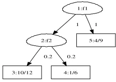
Figure 1: Classification tree: ovals are decisions on a single feature with an associated splitting value. Leaf nodes present a distribution over classes.
5.1. Classification and regression trees
Classification and regression trees [17] use a number of decisions on features to classify each element to one of a number of possible classes (classification) or fit a distribution over a range (regression). An example is shown in Fig. 1. A classification tree (similarly read for regression tree), splits a dataset on a number of features as to make decisions on which class does specific data-points belong to. Internal nodes are decisions, where those data with a value above a threshold on a specific feature go to the right branch and those with values below are placed to the left branch of the decision. Leaf nodes present a distribution over classes that is proportional to the ratio of class data-points at the leaf node. The feature of the root node of the tree in Fig. 1 is
f1and the threshold value is1. In the rightmost leaf node,4examples belong to class
0and9examples belong to class1. Having learned such a tree from training data, it can be used to provide predictions of class for data in which the class is unknown. [12] uses a prior over the set of treesTthat depends on the probability of splitting individual nodes:
ψη =α(1 +eη)−β (2)
p(T) = Y
η∈HI
ψη
Y
η∈HL
1−ψη (3)
whereeη is the depth of nodeη,αandβ are user defined parameters controlling the
size of the trees,HI is the set of internal nodes forT andHLis its set of leaf nodes.
p(T)is the prior probability of treeT andψη is the probability of splitting node η.
(A0) cart(D, Cart) :−
parameters(ψ0, β),
ψ0:: split(0, D, Cart).
(A1) ψH::ψH:: split(EH, DH, c(F, V al, L, R)) :−
parameters(α, β),
EH1isEH+ 1,
ψH1 isα∗EH1−β,
r select(F, V al, DH, DL, DR),
ψH1::split(EH1, DL, L),
ψH1::split(EH1, DR, R).
(A2) 1−ψH::ψH:: split(EH, DH, l(DH)).
(A3) parameters(α, β).
Note that the above program does not contain any guards as the probability labels are calculated within the clauses and are passed via the recursive call via probabilis-tic clauses as defined in Definition 3. Clause (A0) is non-stochastic and serves as a convenient entry point. It is called once at the very start of each invocation and it de-clares thatCartis a valid representation of a tree with prior probability as defined in (3). For each split at depthEH the leaf nodes are considered in turn with a decision
made for each of them as to whether a node is to be split or not. Clauses (A1) and (A2) correspond to the two possibilities. The node will either become an internal one (A1) or a leaf (A2). Note that although the dataDis part of the input to the program, this is purely for populating the tree and has no effect on the probability for each split decision which defines the shape of the tree and the associated prior value.
Clause (A1) states that a sub-tree is initiated at node H by randomly selecting
(r select/5) a featureF and an associated splitting valueV aland using those to
par-tition the dataDH into two distinct partsDLandDR. It then increases the depth by
one, computesψH1 and recursively calls itself onDLandDRproducing the left (L)
and right (R) sub-trees. Clause (A2) constructs a leaf node at levelEH which it
pop-ulates with all data partitioned to this branch. Each time a split is considered (A1) is selected with probabilityψH and (A2) with the complementary probability1−ψH.
For instance, atH = 0 it is the case thatψH = α. The parameters are recorded in (A3). The Dlp program captures the essence of the prior in an elegant and abstract way. SLPs cannot model such a generic prior as they only allow fixed values as labels. The recursive way in which nodes are split has the attractive property that as far as it can go on splitting for ever, the sum of the, infinite, prior is equal to1. In terms of the paths introduced previously this is a case whereπ⊳(Ai) = 1. When applying
probability loss the Dlp program can be changed to perform a one step look-ahead and redistribute the lost mass.
5.2. Bayesian Networks
One approach to constructing the acyclic directed graph for a BN is by recursively choosing parents for each of its nodes as we have shown in [6, Fig. 2]. Care must be taken however as to avoid introducing cycles in the graph. This method is well suited to situations where prior information regarding edges in the graph is available. The top level, non-stochastic part of the selection expressed in logic programming is:
(B1) bn(N ds, BN) :−
bn(N ds, N ds, BN),
no cycles(BN).
(B2) bn([ ], N ds,[ ]).
(B3) bn([N d|N ds], AllN ds, BN) :−
parents of(N d, AllN ds, P a),
BN = [N d−P a|T BN],
bn(N ds, AllN ds, T BN).
Given a list of nodes,N ds, for which we wish to construct a Bayesian network,
BN,predicatebn/2 constructs a candidate graph and then checks that the graph is acyclic. Predicatebn/3 traverses the nodes selecting parents for each one of them. When an ordering is known for the variables in the BN, its construction can proceed without checking for cycles. The ordering constraint [21] specifies that the order of nodes (N ds) is significant and that each node can only have parents from the section of the ordering that follows it.
(B4) bn(N ds, BN) :−
bn(N ds,[ ], BN).
(B5) bn([ ], AllN ds,[ ]).
(B6) bn([N d|N ds], P ossP a, BN) :−
parents of(N d, P ossP a, P a),
BN = [N d−P a|T BN],
bn(N ds,[N d|P ossP a], T BN).
reason why child variables should be selected in order. The following program merges these two ideas:
(B7) bn(N ds, BN) :−
bn(N ds, N ds,[ ], BN).
(B8) bn([ ], All, BN, BN).
(B9) bn(N ds, All, BnSoF ar, BN) :−
p member(N ds, N d, RemN ds),
poss pa(N d, BnSoF ar, All, P ossP a),
parents of(N d, P ossP a, P a),
add(N d−P a, BnSoF ar, N extBnSF),
bn(RemN ds, All, N extBnSF, BN).
The parent node is selected with relative probability (p member/3) from the nodes available. Clause (B9) utilises an auxiliary structureBnSoF arwhich accumulates the graph of the BN at the current level. This is used byposs pa/4 to eliminate cycle-introducing parents which is taken care byadd/3. Clause (B8) terminates the recursion and unifies the auxiliary structure to the BN model. A number of distributions from the literature can be fitted over the edge selection that connects children in the BN to their parents. [24] introducedp(BN)∝κδwhereκis a user defined parameter andδis the number of differing edges/arcs betweenBNand a ‘prior network’ which encapsulates the user’s prior belief about the network structure. [9] suggested a generalisation of the above that allows for arbitrary weights for each missing edge:p(BN)∝P
ijκij
whereiandjrefer to the end nodes of an edge. AssumingW sis a list of pairs matching nodes to weights for parents for this node (W s= [N d1−W1, . . . N dn−Wn] with
Wi = [Wi,1, . . . , Wi,n]) andKnownP ai is the list of parents of theith child in the
prior network, then we have:
(B10) bn([ ], All, W s, KnownBn, BN, BN).
(B11) bn(N ds, All, W s, KnownBn, BnSoF ar, BN) :−
p member(N ds, N d, RemN ds),
poss pa(N d, BnSoF ar, All, P ossP a),
member(N d−N W s, W s),
member(N d−KnownP a, KnownBn),
parents of(P ossP a, KnownP a, N W s, P a),
add(N d−P a, BnSoF ar, N extBnSF),
bn(RemN ds, All, W s, KnownBn, N extBnSF, BN).
(B12) parents of([ ], KnownP a, N W s,[ ]) .
(B13) parents of([P P|P P s], KnownP a, N W s, P a) :−
member(P P, KnownP a),
(B14) parents of([P P|P P s], KnownP a,[Wij|N W s], P a) :−
not(member(P P, KnownP a)),
Wij::parent edge(P P, P a, T P a),
parents of(P P s, KnownP a, N W s, T P a).
(B15) W::W :: parent edge(P P,[P P|T P a], T P a).
(B16) 1−W::W :: parent edge(P P, T P a, T P a).
Clause (B14) utilises probabilistic goal calling by attachingW (Wij) to the goal
parent edge/2. As far as theWijs sum up to1 for a single value ofithe program
leads to no probability loss. This can be enforced by the use of a simple guard that first sums the weights, making sure the add up to1, and then simply selects thejitem from
i’s list. In the context of learning from expression array data [40] constructed tabular priors over the existence of some edges. This is complementary to penalising missing edges. A very similar program to that presented above can capture such knowledge. Other constraints such as the one proposed in [21] where the number of parents is limited can be naturally encoded in our language.
5.3. Likelihood based learning
Bayesian learning methods either look in the posterior distribution for single mod-els that maximise some measure or seek to approximate the whole posterior. The poste-rior over models given some dataP(M|D)is proportional to the prior and a likelihood function,P(M|D)∝p(M)P(D|M). Since the space of all possible models is, in all but trivial examples, too large to enumerate, various approximate methods have been introduced. Variational methods [26] approximate the inference on the evidence by considering a simpler inference task while Markov chain Monte Carlo algorithms sam-ple from the posterior indirectly. In this section we discuss the use of the described priors in a Bayesian model averaging scenario and how this general framework can be used in machine learning tasks on biological datasets.
5.3.1. Metropolis-Hastings
Metropolis-Hastings (MH) algorithms approximate the posterior distribution by making stochastic moves through the model-space. A chain of visited models is con-structed. At each iteration the last model added to the chain, the current modelM, is used as a base from where a new modelM′ is proposed. M′ is stochastically
ac-cepted or rejected. The distribution with whichM′is reached fromM is the proposal q(M, M′)and the acceptance probability is given by
∝ p(M
′)P(M′|D)q(M, M′)
p(M)P(M|D)q(M′, M) (4)
To our knowledge all MH algorithms in the literature have distinct functions for computing the prior and the proposal. Standard MH requires two separate computa-tions. The first is the prior over models: p(M), and the second is a distribution for proposing a new modelM′ from current modelM. The proposed model is accepted
marginal likelihood of the model (measure of goodness of fit to the dataP(M|D)). This often leads to restricting the choices of either the prior [21] or the proposal [12]. Furthermore writing two programs that manipulate the same model-space means that the algorithms are hard to extend to other spaces. The MH algorithm over Dlp requires the construction of a single program, that of the prior.
Our MH scheme follows that of SLPs, which was briefly sketched in [13] and which we then formally introduced in [3]. The main idea is to use the choices in the probabilistic path as points from which alternative models can be sampled. In effect, the resulting MH is a search space constrained algorithm with the proposal reduced to choosing a backtracking strategy rather than defining operations on growing and reduc-ing model structures. Proposals are thus tightly coupled to the prior and take the form of a functionf such thatπM
j =f(πM)whereπM is the path produced for deriving
modelM. πj is the point from whichM′ will be sampled. A consequence of
defin-ing the proposalqin terms of the priorpis that, due to ‘cancelling out’, the quantity
p(M′)q(M,M′)
p(M)q(M′,M) is easy to compute. The acceptance probability (4) is just
p(M′)q(M,M′)
p(M)q(M′,M) multiplied by the likelihood ratioPP((MM′||DD)), so as long as we can compute the likelihood ratio we have an effective MH method which can use any prior defined using Dlp. We will see how likelihoods (and thus likelihood ratios) can be computed for C&RT s and BNs in Sections 5.4 and 5.5 respectively.
Dlp provides a clear connection between computed instantiations and probabilistic choices. The Metropolis-Hasting algorithm can then operate over the priors defined by these programs. Dlp is a powerful probabilistic representation that marries work from the AI community with Bayesian statistics.
5.4. Marginal likelihood for C&RT
Given a particular C&RT classification treeT, letΘ ={θi}ibe the parameters of
the tree, whereθi is the distribution over classes in leafiof the tree. Let(X, Y)be
the data, whereY is to be classified into one ofKpossible classes based on predictor variablesX. The likelihood we need for our MH algorithm is the marginal likelihood
P(Y|X, T), which requiresΘto be integrated out of the full likelihoodP(Y|X,Θ, T). This integration is with respect to the structure-conditional parameter priorP(Θ|T, X), which we define in the standard way. Firstly, we choose to define the prior to be independent ofXso thatP(Θ|T, X) =P(Θ|T). Secondly, we assume independence between theθiinΘ, so thatP(Θ|T) =Qbi=1P(θi|T)whereIis the number of leaves
inT. θi is (pi1, . . . piK): a class probability distribution in T, with pik being the
probability of a sample being of thekth class given that it is placed in theith leaf of treeT. For alli, we setP(θi|T)to the same distribution: a Dirichlet distribution with
parameters(α1, . . . , αK), for some user-defined choice ofαk(1≤k≤K).
With such a parameter prior there is a closed form for P(Y|X, T)as noted by [12]. Letnidenote the number of examples at leafiin treeT. Letnikbe the number
of examples of classk reaching leafi, (so thatni = Pknik). Then the marginal
likelihood is:
p(Y|X, T) =
Γ(P
kαk) Q
kΓ(αk)
b
Y
i=1
Q
kΓ(nik+αk)
Γ(ni+Pkαk)
5.5. Marginal likelihood for BNs
As for C&RT models, we require the marginal likelihood for Bayesian networks (BNs), and so again have to integrate away the parameters. In the case of BNs these parameters are conditional probabilities and we have to define a prior distribution for each of them. We adopt the entirely standard approach of requiring these to be Dirich-let distributions. For the details of this approach see [25]. If various independence assumptions are made about the joint distribution over parameters we have previously shown in the context of Dlp [6, Eq. 5] that for any BNGand observed dataX:
p(X|G) =
n Y
i=1
qi
Y
j=1
Γ(αij)
Γ(nij+αij)
ri
Y
k=1
Γ(nijk+αijk)
Γ(αijk) (6)
whereiranges over the n nodes in the BN,j is a joint instantiation of the parents of such a node in Gand k is a value of the node. nijk is the data count of node
i having value k when its parents have configurationj. αijk is the corresponding
Dirichlet parameter. Finally, nij = Prki=1nijk andαij = Prki=1αijk whereri is
the number of values for theith BN variable. In our past experiments we have set
αijk=N/(riqi),∀i, j, kwhereNis theprior precision) parameter. In the experiments
we reported in [6, Section 4.2] we usedN = 1andN = 10.
5.6. Priors and MH
Using priors for learning statistical models effectively, depends on the structural complexity of the models and the amount of probabilistic bias we wish to impart via the prior. Increased model complexity leads to nondeterministic programs having non-unique probabilistic paths. For instance, the classification trees shown previously are simple recursive structures, the generation of which can be done in a straightforward manner as there are no structural dependencies between the left and right branches of a split node. Thus, the prior program provided was very succinct and it was easy to calculate the probabilities of nodes and leaves. On the other hand, Bayesian networks are more complex as simple programs encoding priors might introduce cycles. As we have shown, guarding against such contextual dependencies leads to more complex programs which are harder to compute with.
Techniques such as using auxiliary arguments can help with unravelling the MH space. Here, we elucidate the effect of priors on MH and explore the difficulties arising in more complex settings.
5.6.1. Classification and regression trees
As detailed above, our approach comprises: a prior, in the form of a Dlp program, an integrated backtracking strategy that proposes new models from old ones and a likelihood which guides the choice between the current and the proposed models. By using a fake likelihood that always returns1 as the ratio of the two models, we can investigate the effect of priors on the proposed models.
2 3
0.8 0.9 1.0 1.1 1.2
alpha a vg. depth beta 0.75 0.8 0.85 0.9 0.95 1 1.05 1.1 1.15 1.2 3 4 5 6
0.8 0.9 1.0 1.1 1.2
[image:20.595.154.454.125.279.2]alpha a vg. lea ves beta 0.75 0.8 0.85 0.9 0.95 1 1.05 1.1 1.15 1.2
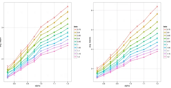
Figure 2: Classification trees prior parameters’ effect on models. Left panel: mean depth. Right panel: mean number of leaves.
of a tree is defined as the length of the longest path from a leaf to the root. The higher the two parameters,αandβ the deeper the trees and the larger the number of their leaves.
We ran3chains of length10,000while varyingαandβ. The range for the two parameters is0.75−1.2with a step increment of0.05. We then count average depth for the trees visited and number of leaves. Having isolated the effect of likelihood, the shape metrics for the trees solely reflect the effect of prior on the chain construction. Figure 2 shows that increasing values for the two parameters increase the depth and number of leaves for the visited trees.
The Dlp described in clauses (A0−A3) succinctly encodes the desired effect from the mathematical description (2 and 3). Furthermore, the probabilistic and logical parts work recursively in tandem. The probabilistic path that pertains to the decisions of constructing the right branch of an internal node is unperturbed by any decision in the left branch. In the terms of (1), ifGP,GLandGRare the goals for the parent, left and
right tree respectively,
PR(GP/θP) =PR(GL/θL)∗PR(GR/θR)
Importantly,θL⊥⊥θRandπ⊳(Ai) = 1. The latter states that within each branch the
sum of probabilities for all possible choices is equal to1thus making the probability of a derivation the exact prior probability of the derived model.
5.6.2. Bayesian networks
Bayesian networks comprise an acyclic directed graph and accompanying condi-tional tables. Here we focus on learning the structure of BNs. Structurally BNs are more complex than classification trees, as the nodes can be connected to each other arbitrarily. Furthermore, the constraint for acyclicity introduces a contextual interpre-tation, in which certain edges lead to invalid models.
1 2 3 4
1 2 3 4
prior’s mean of Gamma
a vg. f amily siz e c=Cyclic, n=BN #=Skew c02 c08 c14 c20 n02 n08 n14 n20 1 2 3 4
1 2 3 4
prior’s mean of Gamma
[image:21.595.144.462.124.289.2]a vg. f amily siz e c=Cyclic, n=BN #=Skew c02 c08 c14 c20 n02 n08 n14 n20
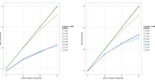
Figure 3: Bayesian networks prior parameters’ effect on models. Left panel: cyclic versus deterministic removal of edges. Right panel: cyclic versus prior using current partial network.
logic fits logic programming well and local probabilistic preferences such as control-ling the average size of (BN) families. Problems arise from the fact that the choice of parents for one node cannot be done without reference to the complete BN structure. Logic for excluding invalid edges can be added either progressively via auxiliary ar-guments that hold the part of the network which has been already constructed, or by removing enough conflicting edges at the end, as to produce a legal BN structure. It both cases though, it becomes difficult to keep the prior probabilities to simple, well understood constructs that map intuitively to the logical components.
To explore the discrepancy between intended prior distribution and actual model metrics we use a naive prior that uses theΓdistribution described by a mean,µ, and skewness parameterκ. The construction proceeds unconcerned by any cycles intro-duced. Those are removed in a deterministic manner by removing edges until an acyclic structure is derived (not shown).
(G2) P :: Γ(µ, κ, X), length(N odes, L), P is(L−1)/X
∼P a::f amily(N odes, µ, κ, P a).
(D1) cyclic bn([], , , ,[]).
(D2) cyclic bn([H|T], µ, κ, N odes,[H−P a|T Cy]) :−
select(H, N odes, P otP a),
f amily(P otP a, µ, κ, P a),
cyclic bn(T, µ, κ, N odes, T Cy).
(D3) P::P::f amily([H|T], µ, κ,[H|T P a]) :−
P ::f amily(T, µ, κ, T P a).
(D4) 1−P::P ::f amily([H|T], µ, κ, T P a) :−
We ran3 chains of length10,000while varyingµ andκ. The ranges for theµ
andκparameters are1−4and2−20with step increments of1 and6respectively. The average family size for the structures visited is then calculated. We first ran the program as shown in clauses (D1−D4), experimentsc02−c20in Figure 3 which produce cyclic structures. The prior was used to construct8-node BNs. We then ran experiments where edges were removed deterministically until a valid BN is reached. The left panel of Figure 3 shows the differential in average family size between the cyclic structures, which faithfully produce networks having average family size equal to the mean of the prior. In contrast, the removal step in the acyclic experiments reduce the average family size. The higher the prior mean the higher the proportion of edges removed as the networks become denser.
We repeated the experiments with an alternative prior in which an auxiliary vari-able held the partial network already constructed. Only candidate edges that do not introduce cycles are considered. For small values of the mean (µ) this prior follows the cyclic distribution closely (Figure 3, right panel). However, asµcomes closer to the number of nodes in the net and the networks become denser, the prior encounters smaller candidate sets from which to chose parental edges that would not introduce a cycle. Thus, the overall objective of a family size ofµcannot be fulfilled.
Writing prior programs for Bayesian network structure is a much harder task than that of composing priors for classification trees. In the cases where cycles are removed from full cyclic networks, the precise probability of a single model is hard to determine as there are multiple paths leading to the same mode. As has been shown experimen-tally the precision of even simple priors on the graphs suffer. When auxiliary arguments are used, the results can be better particularly for reasonably sparse networks. In addi-tion, each structure has a single derivation path.
Although BN priors are complex to characterise mathematically, in practice experi-mentation with unit likelihoods which set the likelihood of every mode to1can provide close enough approximations that can be effectively used for experimenting with con-structing BNs in a specific domain and evaluate the effect of the prior by factoring out the effect of the likelihood.
6. Practical MH
Although Bayesian reasoning is a conceptually simple framework, in practice a number of hurdles have to be cleared before one can use this framework for effective inference. These include expedience of calculations and visiting representative sec-tions of the posterior within a reasonable number of iterasec-tions. Improvements in the literature include parallel tempering [22] and fast likelihood calculations. Tempering is a mixing promoting technique, where a number of chains are run in parallel with swapping moves between chains occurring stochastically. Each parallel chain runs at a different likelihood temperature, a parameter that controls the smoothness of the like-lihood space as to, in turn, control fluidity of chain movement.
choices in the derivation ofM are used as possible backtrack points from which the computation forM′can be embarked on as an alternative probabilistic path. Selecting
these points uniformly can lead to unbiased exploration of the space. As all instanti-ations done forM below the chosen point are undone these type of backtracking can lead to inefficient sampling. Interestingly, the independence of branches in classifica-tion trees with regard toθcan also be exploited to provide more efficient backtracking. Returning to consider the construction of a branch in a tree should leave choices for the other branch unaffected. Executing in a naive fashion would mean that backtracking to a choice in the left branch would remove all choices for the right branch.
A system implementing the main MH algorithm over Dlp priors of model struc-tures as well as advanced feastruc-tures such as declaration of independent paths have been implemented in the Bims system [2]. The system supports expression of Dlp priors, implements a number of in-built likelihoods as well as providing a simple interface for expressing additional likelihoods. The system produces chains of visited models and provides a number of functions for extracting information from such chains. Here we present summaries from two publications that have used priors similar to those presented here.
6.1. Ligand discovery with classification trees
[7] has shown that MH over Dlp scales well and does at least as well as other ma-chine learning algorithms in a cross validation experiment over a large feature space. [7] employed the language and algorithm presented here, to learn the binding affinity of molecules to the pyruvate protein (PYK). Their data were constructed from molecules with known binding affinities from a large NIH funded screening programme. The datasets used contained582molecules from each of the two classes: binders and non-binders to PYK. A high dimensional learning space was constructed by associating each molecule with a large number of features (1572). The study established, by means of a ten-fold cross-validation, that the MH algorithm performed at least as well if not better, in terms of overall accurate prediction of positives, than Support Vector Ma-chines and Feed-Forward Neural Networks. [7] also describes advanced tempering techniques in the context of their experiments.
6.2. Bayesian networks for binding assays
MH over Dlp-defined BN priors was used in [8] to build Bayesian networks (BNs) from binding affinity data on43chromatin proteins. A gamma distribution over par-ents was used with a mean value of1.2for the average family. The dataset comprised
4380measurements and was discretised by setting the strongest5%of protein mea-surements to1and setting the rest to0. The dataset was originally presented in [38] and was analysed using bootstrapping of simulated annealing searches as implemented in the Banjo software for learning BNs [36]. [38] built a consensus network at the80%
7. Conclusions
This paper introduced a general programming language for combining nondeter-minism and probabilistic reasoning in logic programming specially for the purpose of defining prior Bayesian knowledge. The language syntax is presented along with the mathematical concept of probabilistic path that can be used to give semantics in such languages. Furthermore, we focused discussion on how to represent knowledge from the literature.
The paper also presented a characterisation that can be useful in the context of deriving probabilistic information in the form of distributions over variables. This characterisation is of relevance not only to Dlp but also to other generative formalisms that combine logic and probability. We have argued that for certain classes of programs the kind of knowledge that can be represented is substantially expanded. Furthermore, we illustrated via examples on how to write correct and efficient programs that capture knowledge from the Bayesian learning literature.
The main challenges ahead lie in the use of static analysis and program transforma-tions to create programs that exhibit the desirable properties that have been described here, from more arbitrary ones.
We have highlighted that the theoretical framework can compete in producing prac-tical results against standard, well established machine learning approaches. The abil-ity to express prior knowledge can give this approach extra leverage in domains where such knowledge is available.
Availability
The programming language and reasoning techniques described in this paper are implemented in the Bims system which is written in Prolog and freely available from
http://stoics.org.uk/˜nicos/sware/bims. It can be easily installed and
used in two Prolog system:SWI-PrologandY AP.
References
[1] Nicos Angelopoulos.Probabilistic Finite Domains. PhD thesis, City University, London, UK, 2001.
[2] Nicos Angelopoulos. Bims: Bayesian Inference of Model Structure, 2015.
http://stoics.org.uk/˜nicos/sware/bims.
[3] Nicos Angelopoulos and James Cussens. MCMC using tree-based priors on model structure. InProceedings of the 17th Conference in Uncertainty in Arti-ficial Intelligence (UAI), pages 16–23, University of Washington, Seattle, Wash-ington, USA, August 2-5 2001.
[5] Nicos Angelopoulos and James Cussens. Tempering for Bayesian C&RT. In
22nd International Conference on Machine Learning (ICML), Bonn, Germany, August 2005.
[6] Nicos Angelopoulos and James Cussens. Bayesian learning of Bayesian networks with informative priors. Journal of Annals of Mathematics and Artificial Intelli-gence, 54(1-3):53–98, 2008.
[7] Nicos Angelopoulos, Andreas Hadjiprocopis, and Malcolm D. Walkinshaw. Bayesian ligand discovery from high dimensional descriptor data. ACS Journal of Chemical Information and Modeling, 49(6):1547–1557, 2009.
[8] Nicos Angelopoulos and Lodewyk Wessels. Effective priors over model struc-tures applied to DNA binding assay data. In Probabilistic Problem Solving in BioMedicine, (ProBioMed’11), 2011.
[9] Wray Buntine. Theory refinement on Bayesian networks. InProceedings of the 7th Conference in Uncertainty in Artificial Intelligence (UAI), pages 52–60, Los Angeles, California, USA, 1991.
[10] Wray Buntine. Learning classification trees. Statistics and Computing, 2(2):63– 73, 1992.
[11] Soumen Chakrabarti. Dynamic personalized pagerank in entity-relation graphs. InProceedings of the 16th international conference on World Wide Web, pages 571–580, 2007.
[12] Hugh A. Chipman, Edward I. George, and Robert E. McCulloch. Bayesian CART model search (with discussion). Journal of the American Statistical Association, 93:935–960, 1998.
[13] James Cussens. Stochastic logic programs: Sampling, inference and applications. InProceedings of the 16th Conference in Uncertainty in Artificial Intelligence (UAI), pages 115–122, Stanford University, Stanford, CA, USA, 2000.
[14] James Cussens. Parameter estimation in stochastic logic programs. Machine Learning, 44(3):245–271, 2001.
[15] James Cussens. Statistical aspects of stochastic logic programs. InArtificial Intelligence and Statistics, pages 181–186, 2001.
[16] James Cussens. Integrating by separating: Combining probability and logic with ICL, PRISM and SLPs. APRIL project report, January 2005.
[17] David G. T. Denison, Christopher C. Holmes, Bani K. Mallick, and Adrian F. M. Smith. Bayesian Methods for Nonlinear Classification and Regression. Chich-ester: Wiley, March 2002.
[19] P. Domingos and D. Lowd.Markov Logic: An Interface Layer for AI. Morgan & Claypool, 2009.
[20] Nir Friedman, Lise Getoor, Daphne Koller, and Avi Pfeffer. Learning probabilis-tic relational models. InProceedings of the 19th International Joint Conference on Artificial Intelligence (IJCAI), volume 99, pages 1300–1309, 1999.
[21] Nir Friedman and Daphne Koller. Being Bayesian about network structure. In
16th Conference on Uncertainty in Artificial Intelligence (UAI), pages 201–210, 2000.
[22] Walter R. Gilks, Sylvia Richardson, and David Spiegelhalter. Markov Chain Monte Carlo in Practice. Chapman & Hall/CRC, 1996.
[23] Noah D. Goodman, Vikash K. Mansinghka, Daniel M. Roy, Keith Bonawitz, and Joshua B. Tenenbaum. Church: A language for generative models. In Proceed-ings of the 24th Conference in Uncertainty in Artificial Intelligence (UAI), pages 220–229, 2008.
[24] David Heckerman, Dan Geiger, and David M. Chickering. Learning Bayesian Networks: The combination of knowledge and statistical data.Machine Learning, 20(3):197–243, 1995.
[25] David Heckerman, Dan Geiger, and David M. Chickering. Learning Bayesian networks: The combination of knowledge and statistical data.Machine Learning, 20(3):197–243, 1995.
[26] Michael I. Jordan, Zoubin Ghahramani, Tommi S. Jaakkola, and Lawrence K. Saul. An introduction to variational methods for graphical models. Machine learning, 37(2):183–233, 1999.
[27] Minoru Kanehisa and Susumu Goto. KEGG: Kyoto encyclopedia of genes and genomes.Nucleic Acids Research, 28(1):27–30, 2000.
[28] Angelika Kimmig, Bart Demoen, Luc de Raedt, Vitor Santos Costa, and Ricardo Rocha. On the implementation of the probabilistic LP language ProbLog.Theory and Practice of Logic Programming, 11(2-3):235–262, 2011.
[29] Stephen H. Muggleton. Stochastic logic programs. InAdvances in Inductive Logic Programming, pages 254–264. IOS Press, 1996.
[30] Avi Pfeffer. Figaro: An object-oriented probabilistic programming language. Technical report, Charles River Analytics, 2009.
[31] David Poole. Probabilistic horn abduction and Bayesian networks. Artificial Intelligence, 64:81–129, 1993.
[33] Stefan Riezler. Probabilistic Constraint Logic Programming. PhD thesis, T¨ubingen Univ., Germany, 1998.
[34] Taisuke Sato and Yoshitaka Kameya. Prism: A symbolic-statistical modeling language. InProceedings of the 17th International Joint Conference on Artificial Intelligence (IJCAI), pages 1330–1335, 1997.
[35] Taisuke Sato and Yoshitaka Kameya. Parameter learning of logic programs for symbolic-statistical modeling. Journal of Artificial Intelligence Research, 15:391–454, 2001.
[36] V. Anne Smith, Erich D. Jarvis, and J. Alexander Hartemink. Evaluating func-tional network inference using simulations of complex biological systems. Bioin-formatics, 18:s216 – s224, 2002.
[37] The Gene Ontology Consortium. Gene ontology: tool for the unification of biol-ogy.Nature Genetics, 25(1):25–9, May 2000.
[38] Bas van Steensel, Ulrich Braunschweig, Guillaume J. Filion, Menzies Chen, Joke G. van Bemmel, and Trey Ideker. Bayesian network analysis of targeting interactions in chromatin.Genome Research, 20(2):190–200, 2010.
[39] William Yang Wang, Kathryn Mazaitis, Ni Lao, and William W. Cohen. Efficient inference and learning in a large knowledge base.Machine Learning, 100(1):101– 126, 2015.
[40] Andriano V. Werhli and Dirk Husmeier. Reconstructing gene regulatory networks with Bayesian networks by combining expression data with multiple sources of prior knowledge. Statistical Applications in Genetics and Molecular Biology, 6(1), 2007.