Foundations of and Applications for
the Abstract Boundary Construction
for Space-Time
Benjamin Edward Whale
A THESIS SUBMITTED FOR THE DEGREE
OF DOCTOR OF PHILOSOPHY OF
THE AUSTRALIAN NATIONAL UNIVERSITY
Declaration
I certify that the work contained in this thesis is my own original research, produced in collaboration with my supervisor, Prof. Susan Scott; it has not been submitted for any other degree. All material taken from other references is explicitly acknowledged as such.
Ben Whale
Dedication
For Him and her, the centres of my world.
Acknowledgements
Thank you to my supervisor, Prof. Susan Scott. You have provided me with a great deal of support and have always shown a large amount of faith in my ability to tackle the problems that you have given me and that I have encountered. In addition, thank you for your willingness to supervise me while I lived in New Zealand. Your ability to accommodate the changed circumstances of my life, is much appreciated.
Thank you, also, to my two associate supervisors, Dr Ben Andrews and Dr Mike Ashley. Dr Andrews, your technical advice has always been just the right thing to put me back on track and to give me new hope. Thank you for your continued enthusiasm for a subject on the fringes of your own. Dr Ashley, your physical insight has made up for my own lack of training in physics. Your advice on what may or may not work and your ready availability have been important to the completion of this thesis.
To everyone at the University of Canterbury, in particular David Wiltshire: thank you for the money, time and space that you provided me, free of charge. You allowed me to complete my thesis while living in the same country as my wife. For this I owe you much.
To my friends, my wife Karen, my family, and my work colleges, thank you. Al-though none of you really understood what I was doing, and at times you really didn’t want to hear about how I had just devised a new definition of something or other, you have all supported me and desired the best for me. Thank you for being there for me.
Lastly, thank you to all who have contributed to this thesis, but have not been mentioned; in particular, those researchers who have come before and on whose work I have built.
Abstract
The original content of this thesis is comprised of three parts.
First, we investigate the foundations of the Abstract Boundary. We start by pre-senting a one-to-one correspondence between the set of envelopments and a subset of the set of distances on our manifold. This correspondence allows us to define the Abstract Boundary in terms of mathematical structures defined on the manifold, rather than having to use structures additional to the manifold. We take the ideas used in the correspondence and generalise the Abstract Boundary to be applica-ble to any first countaapplica-ble topological space. Then, using the correspondence and the generalisation we give two alternative constructions for the Abstract Boundary. These new methods of construction allow us to bring many new tools to the analysis of the Abstract Boundary and thus enrich the subject and provide new avenues for research.
Second, we discuss how the limiting behaviour of curves relates to the Abstract Boundary. We restrict our attention to the manifold itself and give a classification of the behaviour of curves via the number of limit points they possess. As an application of the classification we weaken the causality assumption of the Abstract Boundary singularity theorem. As an illustration of the problems that curves in a certain class of the classification can cause we give a definition of causality for Abstract Boundary points. In the process of doing so we generalise the distinguishing and strong causality conditions for the boundaries of envelopments and the Abstract Boundary itself.
Third, we investigate the link between the Penrose-Hawking singularity theorems and the Krolak strong curvature condition. We review the singularity theorems and analyse their proofs to determine what can be said about the predicted incomplete geodesics. We see that the conclusions that can be made and the criteria for the Krolak strong curvature condition do not mesh easily. For this reason we present two necessary and sufficient conditions for a geodesic to satisfy the Krolak strong curvature condition, that provide a link between the conclusions and the Krolak condition. The result is that we need to investigate the limiting behaviour of
Contents
Declaration iii
Dedication v
Acknowledgements vii
Abstract ix
1 Introduction 1
1.1 Conventions . . . 1
1.2 Thesis overview . . . 2
1.2.1 Part one . . . 2
1.2.2 Part two . . . 3
1.2.3 Part three . . . 4
1.2.4 Part four . . . 5
1.2.5 Part five . . . 5
1.2.6 Appendix . . . 6
I
Preliminary Material
7
2 Singularities and their legacy 9 2.1 Singularities in general relativity . . . 92.2 The problems of singular behaviour . . . 11
2.3 Boundary constructions . . . 14
2.3.1 The g-boundary . . . 14
2.3.2 The b-boundary . . . 15
2.3.3 The c-boundary . . . 16
2.3.4 The Abstract Boundary or the a-boundary . . . 18
2.3.5 Other boundary constructions and approaches to singularities 20 2.4 An overview of singularity theorems . . . 20
3 A review of the Abstract Boundary 25 3.1 The Abstract Boundary . . . 25
3.1.1 Preliminaries . . . 25
3.1.2 The construction of the Abstract Boundary . . . 29
3.1.3 The classification of boundary points . . . 30
3.1.4 The classification of the Abstract Boundary . . . 34
3.2 The endpoint theorem . . . 37
3.3 The Abstract Boundary singularity theorem . . . 40
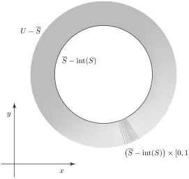
3.4 Partial cross sections . . . 42
II
Foundations of the Abstract Boundary
45
4 The equivalence between distances and envelopments 47 4.1 An equivalence on the set of envelopments . . . 474.2 An equivalence on a class of distances . . . 53
4.3 A correspondence between the equivalence classes . . . 59
4.4 Conclusions and future work . . . 62
5 Boundary sets and sets of sequences 63 5.1 Binary operations on Σ0(M) and their properties . . . 64
5.1.1 Justification for our sequence notation . . . 64
5.1.2 A preorder on Σ0(T) . . . 66
5.1.3 Binary operations on Σ0(T) . . . 67
Contents xiii
5.2 Pseudo-distances on Σ0(T) . . . 75
5.2.1 Induced pseudo-distances . . . 79
5.3 Boundary sets of an envelopment and cauchy sets . . . 86
5.3.1 The covering relation . . . 87
5.3.2 The ‘in contact’ and ‘separate’ relations . . . 88
5.4 Conclusions and future work . . . 91
6 Alternative constructions for the Abstract Boundary 93 6.1 The canonical Abstract Boundary construction . . . 93
6.2 The Abstract Boundary via distances . . . 95
6.2.1 Distance boundary sets and relations . . . 95
6.2.2 The abstract distance boundary . . . 97
6.3 The Abstract Boundary via sequences . . . 99
6.4 Conclusions and future work . . . 101
7 The classification of D(M) 103 7.1 Examples . . . 103
7.1.1 How to make distances that are not in D(M) . . . 103
7.1.2 A distance not induced by a riemannian metric . . . 105
7.2 Constructing an envelopment from a distance . . . 106
7.2.1 Connected components around a boundary point . . . 106
7.2.2 The -neighbourhood approach to construction . . . 108
7.2.3 The endpoint theorem approach . . . 116
7.2.4 Classifying D(M) via chapter 5 . . . 118
7.3 Conclusions and future work . . . 118
8 Curves and their limit points 121
8.1 The limiting behaviour of curves . . . 121
8.2 The classification of curves via their limit points . . . 123
8.2.1 Introductory material . . . 124
8.2.2 The classification . . . 124
8.2.3 |W|= 0 . . . 126
8.2.4 |W|= 1 . . . 127
8.2.5 |W|=|R| . . . 128
8.2.6 Overview . . . 129
8.3 Some examples of winding curves . . . 130
8.3.1 The Carter space-time . . . 130
8.3.2 The Misner space-time . . . 135
8.3.3 Examples of the classification . . . 139
8.4 The Abstract Boundary singularity theorem . . . 140
8.5 Conclusions and future work . . . 141
9 Causal relations for the Abstract Boundary 143 9.1 Causal definitions for boundaries . . . 144
9.2 Causality conditions for the Abstract Boundary . . . 148
9.3 The Abstract Boundary causality relations . . . 154
9.4 Conclusions and future work . . . 155
IV
Physical predictions from singularity theorems
157
10 Consequences of singularity theorems 159 10.1 Theorem 1 of [59] . . . 16010.2 Theorem 2 of [59] . . . 161
10.3 Theorem 3 of [59] . . . 163
Contents xv
10.5 Summary of conclusions . . . 166
10.6 Future Work . . . 168
11 Singularities and the Krolak curvature condition 169 11.1 Proving curvature singularity results . . . 170
11.1.1 The Krolak condition and geodesic divergence . . . 171
11.1.2 Necessary and sufficient conditions for the Krolak condition . 173 11.2 Parallelly propagated vector fields and metric extension . . . 182
11.3 Conclusions and future work . . . 186
V
Summary, Conclusions and Future Work
189
12 Summary, Conclusions and Future Work 191 12.1 Part II . . . 19112.2 Part III . . . 193
12.3 Part IV . . . 194
VI
Appendices
197
A Background results 199 A.1 Topology . . . 199A.2 Curves . . . 200
A.3 Metric spaces . . . 201
A.4 Manifolds and space-times . . . 202
A.5 Surfaces and the second fundamental form and operator . . . 205
A.6 Causality conditions . . . 207
A.7 Divergence and jacobi tensors . . . 209
List of Figures
3.1 The classification of boundary points . . . 32
3.2 Covering table for boundary points . . . 35
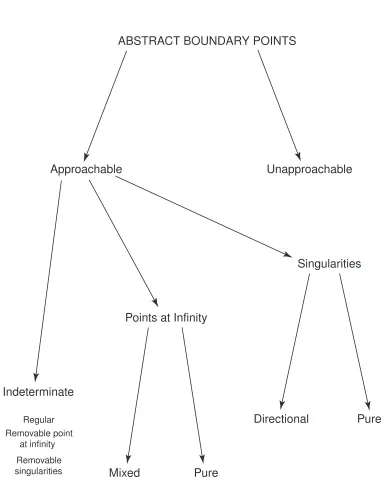
3.3 The classification of Abstract Boundary points . . . 36
5.1 Condition 4 of definition 5.2.1 . . . 77
7.1 A distance not in D(M) . . . 104
7.2 A distance in D(M) that is not induced by a riemannian metric . . . 105
7.3 A manifold with connection number one . . . 107
7.4 A manifold with connection numbers one and four . . . 108
7.5 A manifold with connection numbers one and five . . . 109
7.6 A manifold with connection numbers one and eight . . . 109
7.7 A illustration of the fiber product idea . . . 110
7.8 Attaching fibers to the boundary of an envelopment - finite connection number . . . 111
7.9 Attaching fibers to the boundary of an envelopment - infinite connec-tion number . . . 112
7.10 Pasting together the fibers joined to connection number one boundary points . . . 114
7.11 Using covering space to build -neighbourhood like embeddings . . . . 115
7.12 Using the endpoint theorem to build the envelopment . . . 117
8.1 A summary of the classification of curves by their limit points . . . . 129
8.2 The Carter space-time . . . 131
8.3 The graph of H(t) . . . 133
8.4 The Misner space-time . . . 136
9.1 The new causality relation is not transitive - one . . . 145
9.2 The new causality relation is not transitive - two . . . 146
9.3 The new causality relation is not transitive - three . . . 147
Chapter 1
Introduction
1.1
Conventions
We shall include proofs of theorems in four cases: either, the proof is instructive, we use the details of the proof, the result is not obvious, or the result is original. Throughout this thesis we take our manifolds to be paracompact, connected and hausdorff. We assume that the transition functions between charts are C∞. A Ck
(or Ck−) manifold is a manifold with a metric, g, where g is Ck (or Ck−). Unless
otherwise stated all indices giving components of tensors run across all dimensions. A Lorentzian metric of dimension n is a metric with signature n−2. Thus if our manifold is 4 dimensional a Lorentzian metric would have signature 2 and for any point p∈ M there would exist coordinates so that,
gab(p) =
−1 0 0 0 0 1 0 0 0 0 1 0 0 0 0 1
.
We shall often consider ‘sequences’ or countable subsets of a topological space X as sets; that is as sequences with no ordering. We shall denote any such ‘sequence’ by s, so thats⊂X. For various proofs we shall sometimes need to impose an order on s; in this case we shall write s = {si}i, where we consider that si =f(i) for some
bijective function f : N → s. Technical considerations about ordering only affect the results of chapter 5. In section 5.1.1 we discuss our notation and its justification further.
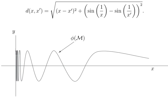
Where unambiguous we shall drop the brackets from expressions like φ(M) and write φM instead. Likewise, when dealing with a function f : X → Y we shall quite happily apply f to both elements of X as well as subsets. For example, if
s = {xi} ⊂ X is some sequence then fs = {f(xi) : xi ∈ s}, or if U ⊂ X then
f U ={f(x) :x∈U}.
Given a function φ : X → Y between two topological spaces we shall often write
∂φX to denote the boundary of the image ofXinY. That is,∂φX =φ(X)−φ(X). We sometimes drop the ◦ from function compositions and write φψ rather than
φ◦ψ.
Let X be a set. Given a function f : [a, b) → X, we will often treat f as a subset of X. For example, given x ∈ X we write x ∈ f meaning x ∈ f([a, b)) and given
g : [c, d)→X we will write f ⊂g rather than f([a, b))⊂g([c, d)).
If X is a topological space we shall denote the set of open neighbourhoods about a point x∈X byN(x). If U ⊂X we shall writeN(U) for the set of open neighbour-hoods of U. If f :X →Y is a continuous map andy ∈Y we shall sometimes write
Nf(y), rather thanN(y), to emphasise that we are using the topology relative toY.
Similarly if U ⊂ Y we shall write Nf(U) for the set of open neighbourhoods about
U inY respectively.
We shall always refer to a metric d : X ×X → R on a topological space as a distance. We do this to distinguish a distance, d : X×X → R, from the metric
g :T M ×T M →R.
1.2
Thesis overview
1.2.1
Part one
The first part of this thesis gives a review of singularities and the Abstract Bound-ary.
Chapter two
We begin by discussing singularity theorems and the need for boundary construc-tions in the analysis of singularities. We spend a while doing this to highlight the distinction between incomplete geodesics and singularities.
1.2 Thesis overview 3
between boundary constructions and try to display the historical development of the ideas behind boundary constructions so that the reader can better understand why the Abstract Boundary is needed and how it arose.
Chapter three
We present here a review of the body of knowledge about the Abstract Boundary that is relevant to this thesis.
1.2.2
Part two
Part two gives the details of two alternative constructions for the Abstract Boundary, that reveal its mathematical structure more clearly than the original construction.
Chapter four
This chapter is the first of the original content, in this thesis. We present a one-to-one correspondence between equivalence classes of the set of envelopments, Φ(M) of a manifold M and a certain subset, D(M), of the set of equivalence classes of topological metrics on the manifold. This chapter lays an important conceptual and mathematical framework for the next three chapters.
Chapter five
Chapter five continues the ideological arguments of chapter four and presents similar material. This time we abstract away from manifolds and distances and work instead only with the set of sequences without limit points and a set, DSeq(M), of functions on these sequences, which parallels the set D(M). In the course of this discussion we show how to construct Abstract Boundary-like sets for any topological space.
Chapter six
show that the Abstract Boundary is fundamentally about sequences and the ‘dis-tance’ between sequences. This in turn shows that the Abstract Boundary straddles the same fine line between topology and analysis as does the study of topological metrics.
Chapter seven
We discuss the important problem of classifying the metrics that belong to D(M). This is a non-trivial problem and we make no attempt to solve it. We do, however, present a number of examples to illustrate metrics that do and do not belong to
D(M), as well as discuss several ways to attack the problem.
1.2.3
Part three
In this part we discuss the relationship between curves and the Abstract Boundary. Our motivation is to better meld the physical content of space-times with the Ab-stract Boundary as well as to illustrate a particular problem that can occur. We give two examples by strengthening the Abstract Boundary singularity theorem and by defining the past/future of Abstract Boundary points.
Chapter eight
We begin by discussing the importance and behaviour of ‘winding’ curves. We present a number of results pertaining to the classification of curves by the number of accumulation points they possess and then use them to improve the Abstract Boundary singularity theorem.
Chapter nine
1.2 Thesis overview 5
1.2.4
Part four
In part four we build on the research program suggested by Ashley and Scott in [5], by investigating the problem of the physical properties of the incomplete geodesics predicted by the singularity theorems in [59]. While the material here does not directly refer to the Abstract Boundary, it is none-the-less intimately connected via the material in [5].
Chapter ten
We start by reviewing the details of the Penrose-Hawking singularity theorems. By analysing their proofs we are able to make a handful of conclusions about the prop-erties of the predicted incomplete geodesics. We discuss these conclusions within the context of the increasing strength and the physicality of each singularity theorem’s assumptions. We finish the chapter by suggesting a set of conditions with which to start investigation of the physical properties of the predicted incomplete curves.
Chapter eleven
By comparing the conclusions of the singularity theorems, derived in chapter ten, to the Krolak strong curvature condition we observe that there is a problem with fitting them together. To solve this problem we prove necessary and sufficient conditions for a geodesic to satisfy the Krolak strong curvature condition. This reduces the problem of connecting physical properties to predicted incomplete geodesics to an analysis of the limiting behaviour of a single divergence along the geodesic. We then give a preliminary result which shows that maximal extension of a metric is related to the behaviour of parallelly propagated frames. Future work, linking parallelly propagated frames and jacobi fields would allow us to derive the necessary results about the limiting behaviour of divergence along geodesics.
1.2.5
Part five
Chapter twelve
1.2.6
Appendix
Appendix A
Part I
Preliminary Material
Chapter 2
Singularities and their legacy
2.1
Singularities in general relativity
Singularities are a general feature of physics. A common example comes from clas-sical electrodynamics. The potential of an electric field generated by an electron has the form 1r, in polar coordinates. This potential diverges to ∞ as we let r go to 0. We can say that the potential tends to infinity in finite parameter length. Typically, this behaviour is called singular and the origin is called the singularity. Think of the potential as ‘containing’ the singular behaviour and the polar coordinates as ‘describing’ the behaviour.
In general relativity we see similar behaviour. This behaviour, however, has one very important difference from other classical physics theories. In general relativity the mathematical object that contains the singular behaviour is intimately connected to the object that describes the behaviour. In the example above the object that contains the singular behaviour is the field, 1
r, but the object that describes the
behaviour is the background space; in 4 dimensions it could beR4 plus a Lorentzian metric, g, that describes distance (among other things). In general relativity the mathematical object that contains the singular behaviour is the metric, g, itself. This causes substantial problems, indeed the majority of this thesis is about devel-oping mathematical tools to adequately deal with these problems.
As mentioned general relativity uses a Lorentzian metric on a manifold to describe space-time. By definition, the metric must be non-degenerate on the manifold. This means that the metric must be well-behaved at all points on the manifold, or that there are no points that are ‘singular’. There may be singular behaviour, but there are no points which can be called singular. It is this issue which causes the mathematical problems relating to singularities in general relativity.
To clarify I shall illustrate our two examples in more mathematical detail.
First, the case of a simplified electric field generated by an electron. The underlying manifold isR4and we choose Euclidean coordinates, (t, x, y, z)1. The object with the singular behaviour is a function from R4 to R, defined by f(t, x, y, z) = √ 1
x2+y2+z2. Note that the singular behaviour occurs as we limit to the origin and that the origin forms part of the mathematical structure.
Second, the case of the gravitational potential inside a non-rotating, non-charged, black hole, called the interior Schwarzschild space-time. Let m ∈ R, then the manifold is B3\{origin} ×R (whereB3 is the three dimensional ball) and we choose Euclidean coordinates, (t, x, y, z), so that 0 < px2+y2+z2 < 2m. The object with the singular behaviour is the metric, g, which in these coordinates takes the form −
1− √ 2m x2+y2+z2
0 0 0
0
1− √ 2m x2+y2+z2
−1
0 0
0 0 x2+y2+z2 0
0 0 0 (x2+y2+z2) sin2θ
In this case we can see that the metric has components that tend to 0 and ∞
as px2+y2+z2 tends to 2m and to 0. These are an examples of singular be-haviour. Unlike the previous example, even though the singular behaviour occurs as px2+y2+z2 tends to 2m and 0 the points (t, x, y, z), where p
x2+y2+z2 is equal to 0 can not be part of the mathematical structure; if they were the function
g would be degenerate and hence not be a metric. This same fact is not true for the points (t, x, y, z), wherepx2+y2+z2 is equal to 2m. By choosing different coordi-nates, it is possible to define a metric on a larger manifold than extends g through these points [74]. This is an example of what is called a coordinate singularity: the singular behaviour is a figment of our own construction, via our choice of coordi-nates. This neatly illustrates that the study of singular behaviour can be complex. See [16] and either [19] or [45] for further examples of coordinate singularities.
To summarize: for the first example the singularity is a part of the mathematical structure and in the second example it is not. This is forced on us by the definition of the objects that contain the singular behaviour.
1
2.2 The problems of singular behaviour 11
We have seen that there can be no singularities in general relativity, in the usual sense. This does not, however, mean that we can ignore ‘singular behaviour’. Indeed by virtue of singularities influencing physical behaviour near by it, we are compelled to examine the singular behaviour near them, see [45]. The study of singular be-haviour in general relativity comprises of two problems; location and definition. I shall continue this chapter by discussing and illustrating both problems.
2.2
The problems of singular behaviour in general
relativity
The obvious approach to studying singular behaviour is to use limits. This can be done by using a chart to describe the direction of the limit. Unfortunately, this raises the problem of location.
The limiting location of singular behaviour, studied via a particular chart, is co-ordinate dependent. For example, in the interior Schwarzschild space-time we can analyse the singular behaviour via the two limits r →2m, t = 1, φ= π
2, θ =
π
2 and
r →2m,t = 1, φ= 3π
2 , θ=
π
2. This gives us the behaviour as we approach the differ-ent coordinate points (2m,1,π2,π2) and (2m,1,π2,32π). Alternatively, we can analyse the singular behaviour in the coordinates, t, r0, θ, φ where r0 = r−2m. Under this transformation the two limits above become the limits r0 → 0, t = 1, φ = π
2, θ =
π
2 and r0 → 0, t = 1, φ = 32π, θ = π2. In this chart we study the behaviour as we ap-proach the two points (0,1,π
2,
π
2) and (0,1,
π
2, 3π
2 ), which (because of the polar nature of the r0 coordinates) are both the same point. Thus, in two different charts, the ‘same’ limits give different locations for the singular behaviour. In one chart we lo-cate the singular behaviour at two different locations, (2m,1,π2,π2) and (2m,1,π2,32π), in the other chart the singular behaviour is located at one location (0,1, θ, φ). This is a simplistic example. In many cases the location of the singular behaviour under different coordinates is not as clear as in this example, see [98, 97]. We need to find some way to describe the location of singular behaviour that accounts for changes of coordinates, or a definition of the location of singular behaviour that is coordinate invariant. This is the problem of location.
To clarify we will again use the interior Schwarzschild example. As originally pre-sented in the coordinates (t, r, θ, φ) the metric took the form
− 1− 2m r
0 0 0
0 1− 2m r
−1
0 0
0 0 r2 0
0 0 0 r2sin2θ
The metric seems to have singular behaviour towards r = 2m and r = 0. There is, however, no pathological behaviour for r = 2m. We can express the metric in a different chart. Let,
r∗ =
Z 1
1−2m r
dr
=r+ 2mlog|r−2m|
and define v =t+r∗. We shall use new coordinates (v, r, θ, φ) in which the metric is given by,
− 1− 2m r
1 0 0
1 0 0 0
0 0 r2 0 0 0 0 r2sin2θ
which we can see has no singular behaviour towards r= 2m.
We can define a new space-time with manifoldR3\{origin}×Rand with coordinates
v, r, θ, φ where 0< r and the metric is
− 1− 2m r
1 0 0
1 0 0 0
0 0 r2 0 0 0 0 r2sin2θ
Then the region given by 0< r <2m is diffeomorphic to the interior Schwarzschild space-time. The singular behaviour of the Schwarzschild space-time at r= 2m has thus been shown to be a result of a bad choice of coordinates.
2.2 The problems of singular behaviour 13
definition: when does singular behaviour lead to the existence of a singularity? Some further discussion can be found in [42].
There have been two principle approaches in the literature to these problems. The first is to approach them on a case-by-case basis, to analyse each space-time indi-vidually using properties of the space-time to build understanding of the singularity. See [25] for an advocation of a sophisticated example of this approach or [97] and [98] for a more constructive example. The second is to find a ‘universal method’, which can be applied to any space-time, for example, [99].
The first approach is useful. Its main flaw is that, by considering each space-time separately, the definition of what constitutes singular behaviour can change. In addition, for any particular space-time, what is and is not singular behaviour is somewhat open to interpretation.
The second approach, avoids the ambiguity created by a case-by-case analysis by providing a general construction applicable to a wide class of space-times. The usual approach, [42, 44, 94], is to attach boundary points to the manifold to give a unique location for the singularity. This can be problematic. In the Schwarzschild space-time, should we represent the singularity at the origin as a point, or a sphere, or some other surface? In the case of complicated space-times, such as the Curzon space-time ([98, 97]), one choice of points cannot do justice to the full range of singular behaviour and so by attaching points to the manifold we can unnecessarily complicate the study of singularities.
The Abstract Boundary [99] avoids both of these problems by giving a prescription of the location of a singularity that allows for re-expression of its location in any coordinates. So that in one representation the singularity is a point and in another it is a surface.
Of course all of this is not quite as black and white as we have discussed above. For singularities that are a subset of what Ellis and Schmidt, [31], called ‘quasi-regular singularities’, the local structure is such that a well defined notion of location can be given without reference to any boundary construction [115]2. Hence the problem of location is readily answered in this particular case. In addition, Vickers has discussed such singularities within the context of cosmic strings and distributional solutions to Einstein’s field equations [105, 114, 115, 116]. The result is an answer to the problem
2
of definition: Such singularities should be seen as physical objects. None-the-less, in the majority of cases, boundary constructions are needed to properly work with singular behaviour. Indeed in [116] Vickers uses the b-boundary to analyse a larger class of quasi-regular singularity and in [115].
We now discuss the most common boundary constructions from the point of view of the problems of location and definition. We do not give a detailed overview since two excellent reviews already exist, see [3] and [101].
2.3
Boundary constructions and the problems of
location and definition
2.3.1
The
g
-boundary
The g-boundary [41] attaches a point to the end of every incomplete geodesic in the space-time. The set of all of these points by∂g. The elements of ∂g are identified via
an equivalence relation so that the space-time with attached points satisfies certain topological properties. When the space-time is maximally extended every point of
∂g is classified as a singularity [41].
The g-boundary, as originally given, attempted to specify a unique boundary for any space-time. Further investigation [43] has shown, however, that the equivalence relation given in [41] produces unsatisfactory topological properties in some simple space-times.
There are a number of problems with theg-boundary. Firstly, in [42] Geroch presents a space-time with no g-boundary which contains an incomplete causal curve. The presence of this curve shows that the space-time contains singular behaviour and yet no g-boundary singularities. This shows a failure of the g-boundary to answer the problem of location.
The g-boundary fails to answer the problem of definition, by defining all elements of ∂g to be singular points, for a maximally extended space-time. As we shall see in
2.3 Boundary constructions 15
None-the-less theg-boundary was an important step in the development of boundary constructions. Geroch showed that it was possible to construct such a boundary and he also demonstrated its importance, [41, 42].
For more information about the problems of the g-boundary refer to [3, 41, 42, 43].
2.3.2
The
b
-boundary
The b-boundary [92] constructs a topological metric on the bundle of linear frames over the space-time and uses the continuous action of a group on the bundle to create a projection from the cauchy completion of the bundle to a manifold. By construction, this new manifold contains the original space-time as an open dense set.
This construction gives a uniquely determined boundary, ∂b. For example there is
no choice of an equivalence relation. Each boundary point is located at the end of an incomplete curve and every incomplete curve ends at a boundary point, [92]. A singularity is a pointp∈∂b that is an element of∂b for all extensions of the manifold,
[92]. Because of these properties the b-boundary solves the two main problems of the g-boundary, mentioned above.
Where the g-boundary does not include enough boundary points, however, the b -boundary includes too many. In particular, incomplete curves that are contained in compact regions (such as occur in the Misner space-time) should not end at singularities, since these singularities will not be T1 separated from the limit points of the curve, see theorem 5.1 of [92]. In addition Johnson, [65], has shown that the b-boundary gives non-Hausdorff behaviour for a large class of spacetimes, which includes both the Schwarzschild and Friedmann solutions. The acceptance of such behaviour is an ideological position, see [50, 51]. Geroch, Penrose and Kronheimer, [44], have stated that
“...since so little is known at present about the details of the structure of space-time singularities, one would like to have techniques that can - in principle, at least - cope with virtually any type of situation consistent with the requirements of causality.”
The b-boundary also suffers from another problem. It identifies singularities which, due to physical properties, are better considered to be separate, see [14, 15, 65, 66]. One example is the identification of the past and future singularities of the FRW cosmology. Hence theb-boundary’s answer to the problem of location is inadequate. Theb-boundary answers the problem of definition by defining all points of∂bthat are
an element of∂b for all extensions of the manifold to be singularities, [92]. In addition
there is a classification of these singular points based on the limiting behaviour of the metricgand related tensors and scalars, [31]. While adequate, we shall see in chapter 3 that more detail can be added to this definition of singularity. We note in passing that the classification given in [31] can be adapted to the essential singularities of the Abstract Boundary. Hence, while theb-boundary does an adequate job of answering the problem of definition the Abstract Boundary provides a more nuanced approach. It is worthwhile noting that Dodson [28, 29] and Slupinski and Clarke [102] have attempted to modify the definition of the b-boundary to avoid the problems men-tioned above. These new constructions, however, suffer from other criticisms, see [3] for a discussion. A great deal of work has been done on/using the b-boundary. For more information please refer to [3, 14, 15, 23, 25, 28, 29, 30, 43, 49, 52, 61, 62, 65, 66, 95, 93, 94, 102, 103, 104, 113].
2.3.3
The
c
-boundary
Thec-boundary uses the causal structure of the space-time to define a boundary [44]. A future (past) set C is a set so thatI+(C) =C (I−(C) = C). An indecomposable future (past) set is a future (past) set that is not the union of at least two proper subsets that are also future (past) sets. In any distinguishing space-time there exists a correspondence between the set of points in the space-time and a subset of all future (past) indecomposable sets. The set of all future (past) indecomposable sets can be given a topological structure and by using the (above-mentioned) correspondence the space-time can be homeomorphically mapped onto its image. The points in the set which are not in the image of the map are called the future (past)c-boundary, ∂f c
(∂p
c). In order to create a single boundary for the space-time an equivalence relation
is used to identify elements of ∂cf and ∂cp.
In [44] we are given the theorem:
2.3 Boundary constructions 17
Thusc-boundary points are located at the ends of causal curves, which do not have endpoints in the space-time. The paper [44] does not give an explicit definition of a singularity. It does imply, however, that the g-boundary can be classified into singular points and points at infinity.
The equivalence relation given in the originalc-boundary paper [44] gives unphysical and unintuitive answers in many simple space-times [75, 79, 107, 76]. This has led to some debate as to the correct form of the equivalence relation and the necessity to use a topology, [17, 54, 77, 79, 86, 107, 108]3. To date, however, there is no strong evidence for choosing any particular relation over any other, as similar problems have been found with these suggestions [34, 77, 79, 76]. In the very recent paper [34] Flores has claimed to have produced a construction in which, “...all previous objections disappear”. Certainly Flores has shown that his construction gives suitable results on many standard examples, but the construction is not necessarily unique, see theorem 7.2 of [34]. In addition it is yet to be seen if new examples can be given which show that Flores’ construction suffers from similar problems as those in [17, 86, 79, 107].
In addition to this ambiguity, as thec-boundary ascribes an endpoint to every causal curve, it suffers from the similar non-T1 behaviour as the b-boundary. While it is possible to remove these points directly from∂c, as is done in [34], this behaviour may
indicate an underlying problem, depending on one’s idealogical position regarding precompact incomplete geodesics, see chapter 8. Hence on these two counts the
c-boundary fails to give an adequate answer to the problem of location.
There is no systematic classification ofc-boundary points. There is, however, no the-oretical impediment to applying a similar classification as used in the b-boundary. In [44] the authors discuss singular c-boundary points of the Schwarzschild space-time, by an appeal to the incompleteness of geodesics. In [107] ‘naked’ boundary points are defined through an appeal to the structure of TIP’s and TIF’s. This indicates that a more thorough classification maybe possible. Hence, while the c -boundaries answer to the problem of definition is deficient this is probably due to lack of research.
3
Development of the c-boundary still continues. For further reading consult [1, 2, 3, 17, 20, 24, 34, 35, 53, 54, 55, 56, 68, 77, 75, 79, 86, 87, 91, 100, 108] and the references therein.
2.3.4
The Abstract Boundary or the
a
-boundary
Unlike the previous boundaries the Abstract Boundary [99] makes no unique choice of boundary. Rather it asserts that any topological embedding, φ : M → N (dim M= dim N), gives a viable boundary, ∂φ = φM −φM. This means that a
boundary is constructed for every such embedding of the manifold. An equivalence relation is formed on the union of all subsets of each boundary. This allows us to construct the abstract boundary, B(M). An element of B(M) is an equivalence class of a point in a boundary ∂φ = φM − φM for some φ : M → Mφ an
em-bedding where Mφ is of the same dimension as M. Each subset in the equivalence
class expresses the same information but in a different way.
There is an interesting analogy (that only goes so far!) between vectors and el-ements of B(M). Let v be a vector in R2, in different coordinates v could be represented as (0,0),(1,2),(π, π2) or any other ordered pair. We can consider v as the set of all ordered pairs, that in a given coordinate system represent v. So that
v = {(0,0),(1,2),(π, π2), etc...}. In fact, this is a way of representing vectors, as an equivalence class on the set of all ordered pairs of all coordinates on R2. So, just as elements of the equivalence class corresponding to v tell us different infor-mation about v, so too do elements of an equivalence class ofB(M) tell us different information about that element of the boundary. We can think of embeddings as coordinates and elements of B(M) as vectors.
As mentioned this analogy only goes so far. For example an element of the Abstract Boundary might not have a representative in a particular embedding, while a vector will always have a representation in a particular coordinate system.
It is remarkable that such an all encompassing structure as B(M) can give us any information at all, let alone answers to the problems of location and definition. The
2.3 Boundary constructions 19
points are points through which it is possible to extend the manifold and connection, in some embedding. This classification is dependent on a choice of preferred curves, such as affinely parameterised causal geodesics, or causal curves with generalised affine parameter.
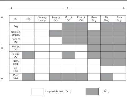
The abstract boundary does not suffer from the same issues as the g, b or c -boundaries. It does, however, have its own problems, but unlike the other boundaries they are to do with calculation, rather than the ideology behind its construction. Firstly, due to its definitionB(M) is impractical to compute since it requires knowl-edge of all possible embeddings of the manifold. There are, however, a number of results (see figure 3.2) that can be used to gain information about B(M) without explicitly constructing it. Examples of how these results are used can be found in [85]. In part II we give an alternative construction of the Abstract Boundary that, although not solving this problem, will allow for easier applications in some situations.
Secondly, because boundary points are located at the end of sequences, rather than curves, the curves that create the non-T0 behaviour in other boundary constructions cause different problems, in certain situations. For example if we have a precom-pact incomplete geodesic γ to which a boundary point p is associated then in any reasonable topology on the manifold union boundary the pointpwill be non-T0 sep-arated from the limit points ofγ. When there exist two embeddingsφ1 :M → Mφ1 and φ2 : M → Mφ2 so that for some curve γ, φ1(γ) has multiple limit points in
∂(φ1(M)) but φ2(γ) has only one limit point in∂(φ2(M)), we see the ghost of this non-T0 behaviour affect the a-boundary. These problems have to do with the inter-play between the limiting behaviour of these curves and of sequences on the curves. We discuss this problem and give more complete examples in part III.
Thirdly, because the classification of boundary points depends on a choice of pre-ferred curves it is possible for the same boundary point to have a different classifi-cation for different choices of curves. This is subtly different from the issue of the choice of an equivalence relation in theg and c-boundary. For the g andcboundary the choice of curves was used in the construction of the boundary, while for the
causal curves with generalised affine parameter with no ill effects.
2.3.5
Other boundary constructions and approaches to
sin-gularities
There are a number of other boundary constructions. The most notable of which are the atlas or A-boundary of Clarke, [26], the causal boundary (as distinct from thec-boundary) of Garcia-Parrado and Senovilla [36, 37, 38, 39, 40] and the singular cauchy boundary of Gruszczak, Heller and Pogoda [47, 48].
We do not discuss these boundaries here, either because they are rarely used in the literature (the A-boundary is used for one theorem in [26], see page 51), are very new and use a similar ideology as the a-boundary (the causal boundary [37]) or are very similar to the b-boundary (the singular cauchy boundary [49]).
2.4
An overview of singularity theorems
When the first solutions to Einstein’s field equations were found to have singular-ities, people thought that these were due to the very high level of symmetry built into these solutions [7, 59, 101]. In 1955, however, the first singularity theorem was published by Raychaudhuri [88], and independently confirmed in 1956 by Komar [69] (see [101]). These theorems depended on precise forms of matter, however, and so the debate about the existence of singularities continued. After the subject had developed enough tools to handle the global properties of space-times, Penrose published the first ‘modern’ singularity theorem [83]. This was quickly followed by singularity theorems due to Hawking, Geroch, Ellis and others, see [113]. These results showed that there must exist incomplete causal geodesics, if certain general properties of matter and of the universe were satisfied. Due to the issues discussed in section 2.2 we know that, without a proper definition of a singularity, one cannot prove that incomplete geodesics imply that there must be a singularity. Nonetheless, geodesic incompleteness is usually assumed to be a sufficient indicator of the exis-tence of a singularity. Hence theorems of this sort are called singularity theorems and are usually assumed to show that singularities are a generic feature of solutions to Einstein’s field equations4, see page 750 of [101] for further discussion.
4
2.4 An overview of singularity theorems 21
Here we review the more famous of the singularity theorems, in order to give the reader some idea of the importance of them. Since we cover the details of four of the modern singularity theorems in part IV we only give an outline of the field here. Each of the singularity theorems has three basic assumptions; firstly, an assumption about the nature of matter, secondly, an assumption about causality and thirdly, an assumption about initial or boundary conditions of the collapse or expansion. Of course each of these assumptions is open to debate and much work has gone into weakening them, see [10, 11, 12, 13, 22, 67, 78, 89, 90, 101, 109, 113, 111] and the references therein.
As mentioned previously, the first singularity theorem was proven, independently, by Raychaudhuri in 1955, [88], and Komar in 1956, [69]. Here we state a modern version of their result from [101].
2.4.1 Theorem. Assume that the matter content of the space-time can be described by an energy-momentum tensor of the perfect fluid type and that the velocity, u of the fluid is geodesic (non-accelerating) and irrotational. If the expansion is positive at an instant of time and the energy condition R(u, u) ≥ 0 holds, then there is a matter singularity in the finite past along every integral curve of u.
This theorem is specialised; however, it makes few assumptions about the geometry of the space-time. At the time this was an important theorem to counter the claims that singularities arose as a result of symmetry.
This theorem also relied on what is now known as the timelike Raychaudhuri equa-tion,
d
dτθ =−Ric(γ 0, γ0)
−tr(ω2)−tr(σ2)− θ 2
n−1
This equation relates the expansion (θ), vorticity or rotation (ω), and shear (σ) of a congruence of timelike geodesics (γ) to the curvature of space-time (τ is the affine parameter of the congruence and n is the dimension of the space-time). It can be derived from the geodesic deviation equation, although when this result was first published that was not the route followed. Note that there is also a version of the Raychaudhuri equation for null geodesics.
in geodesics and therefore also to the proofs of the singularity theorems. Refer to the proofs in section 10 for examples of this relationship.
This singularity theorem differs from the others in one important regard; it makes specific claims about the nature of the singularity and where it is located. It is an interesting feature of singularity theorems, that the more general they are, the less specific the result becomes with regards to the nature of the singularity.
Singularity theorems that use global techniques to derive the existence of an incom-plete geodesic are often referred to as ‘modern’ singularity theorems.
The first of these was proved by Penrose in [83]. We present here the version in [59, pg 273].
2.4.2 Theorem. A space-time (M, g) cannot be null geodesically complete if
1. for all null vectors v, R(v, v)≥0,
2. there exists a non-compact cauchy surface H in M,
3. there exists a closed trapped surface T in M.
This theorem generated allot of further research, along similar lines, see [113] for a review. The idea behind the proofs of all of the majority of these theorems is the same. It goes as follows: assume that the space-time is null/timelike/non-spacelike geodesically complete; show that some set (D+(S), E+(S), . . .) is compact by using the convergence condition, energy condition, the Raychaudhuri equation and the completeness of the class of geodesics to show that along some congruence each geodesic must have a conjugate point a finite distance in the future or past; then use the causality condition to show that there is a contradiction.
This theorem makes no claims as to the nature of the singularity. Some information, however, can be found after an analysis of the proof. This information is much less revealing than for the Raychaudhuri-Komar result, but is still useful. See part IV. As mentioned above, Penrose’s theorem sparked a great deal of interest in similar results. Most of which involved weakening one or more of the conditions, see above for a list of references. An excellent example was proved by Maeda and Ishibashi in 1996, [78].
2.4 An overview of singularity theorems 23
1. Every endless causal geodesic (a geodesic with an affine parameter defined for all of R) has a pair of conjugate points.
2. The space-time is not totally vicious and, if the chronology condition fails at the set V ⊂ M, then either,
(a) There exists p ∈ ∂V such that for all U ∈ N(p) and all closed future-directed timelike curves, γ, intersecting V ∩U, there exists a compact set
K so that γ ⊂K, or
(b) for all p ∈ V and all q 6∈ I+(p) ∩ I−(p) the set (∂J+(q)∩∂J−(q)) ∩ (I+(p)∩I−(p)) is not empty.
3. There exists a trapped set.
In this theorem the energy condition has been replaced by 1. This can be done because the energy condition in a singularity theorem is usually used to prove some thing similar to 1 via the Raychaudhuri equation. Statement 2 is a rather technical condition about the exact nature of causality violation. It is much weaker than the usual causality condition used because it only deals with violation of the chronol-ogy condition, while most other singularity theorems assume the strong causality condition. We can see here that, without increasing the strength of the other two conditions, the causality condition has been significantly weakened.
There are cosmologies that violate the energy conditions assumed by most singularity theorems. Some work has been done to mitigate this problem, see [9, 67, 110]. Most notably the strong energy condition can be replaced by the weak energy condition and/or an averaged strong energy condition. Namely, that
Z
R(γ0, γ0) dτ ≥0
along a geodesic γ and where
Z
R(γ0, γ0) dτ = 0
only if R(γ0, γ0) = 0 everywhere onγ.
Lastly, there are a number of results that exploit gravity waves to show that singu-larities can form in vacuum solutions to Einstein’s field equations. This theorem is taken from [112]; refer to [46] for a thorough review.
2.4.4 Theorem. Suppose that a space-time contains two global space-like killing vectors ξ2 and ξ3 acting on space-like surfaces with R2 topology. Take a
pseudo-orthonormal basis k, l, ξ2, ξ3 and assume that at least one of the Newman-Penrose
quantities σ, λ,Ψ0,Ψ4,Φ00,Φ22 is non-zero at some point p ∈ M. If ξi, i= 2,3 is
tangent to a partial Cauchy surface Σ 3 p which is non-compact in the spacelike direction orthogonal to ξi, and the null convergence condition holds, then Mis null
geodesically incomplete.
Chapter 3
A review of the Abstract
Boundary
This chapter reviews the aspects of the Abstract Boundary needed for the rest of the thesis. We do not attempt to give a thorough overview. For those that are interested, please refer to the papers [4, 5, 32, 33, 99]. There is also additional material in Ashley’s PhD thesis [3] and Philpot’s honours dissertation [85].
As mentioned earlier the Abstract Boundary takes a very different ideological ap-proach to the construction of a boundary. It still attempts to answer the problems of location and definition, but it does so in a very different way. After giving the definition we shall discuss how the Abstract Boundary answers these two problems.
3.1
The Abstract Boundary
In this section we present the Abstract Boundary. Apart from a few remarks and a definition, this section is a condensed version of the paper [99].
3.1.1
Preliminaries
Embeddings and boundary sets
This subsection covers the necessary definitions and results for the construction of the Abstract Boundary. We begin by defining an envelopment, move on to boundary sets and lastly define an equivalence relation on boundary sets that will allow us to construct the Abstract Boundary.
3.1.1 Definition. Let M and M0 be manifolds of the same dimension. If there
exists φ :M → M0 a C∞ embedding, then M is said to be enveloped by M0, M0
is the enveloping manifold and φ is an envelopment. Since both manifolds have the same dimension, φMis open inM0.
3.1.2 Definition. A boundary point of an envelopment φ : M → Mφ is a point
p∈∂φM. A boundary set of an envelopment is a non-empty set B ⊂∂φM.
We are now in a position to define a partial order (the covering relation) on the set of all boundary sets of all envelopments. This partial order is used to construct the equivalence relation necessary to form the the Abstract Boundary.
3.1.3 Definition. Let φ : M → Mφ and ϕ : M → Mϕ be envelopments. Let
Bφ be a boundary set of φ and Bϕ a boundary set of ϕ. Then Bφ covers Bϕ or
equivalently BφBϕ if for every U ∈ Nφ(Bφ) there exists V ∈ Nϕ(Bϕ) so that,
φϕ−1(V ∩ϕM)⊂U.
When either of the boundary sets is a singleton {p}we shall write pB rather than
{p}B.
Before we give the equivalence relation, there are a number of important results about the covering relation that we shall need later.
3.1.4 Theorem. A boundary set B covers a boundary set B0 if and only if B covers every point p∈B0.
3.1.5 Theorem. A boundary set Bφ ⊂ ∂φM covers another boundary set Bϕ ⊂
∂ϕMif and only if for every sequence{xi} ⊂ M so that{ϕxi}has an accumulation
point in Bϕ, the sequence {φxi} has an accumulation point in Bφ.
Given the importance of this theorem in part II of this thesis, we provide an outline of the proof.
Proof. Assume that BφBϕ. Suppose that {xi} is a sequence in M so that {ϕxi}
has an accumulation point in Bϕ. Choose some nested collection of open sets
Ui ∈ Nφ(Bφ) so that
T
Ui = Bφ then using the covering condition it is possible
to construct a subsequence {yi} of {xi}so that {φxi}has an accumulation point in
3.1 The Abstract Boundary 27
Assume that Bφ 6Bϕ. Then there existsU ∈ Nφ(Bφ) so that for all V ∈ Nϕ(Bϕ),
φϕ−1(V ∩ϕM)\U 6=∅. This condition can be used to construct a sequence{xi}so
that {ϕxi}has an accumulation point in Bϕ but {φxi} has no accumulation points
in Bφ.
We are now able to define the necessary equivalence relation.
3.1.6 Definition. Given two boundary sets, B, B0, ifBB0 and B0B thenB is
equivalent to B0 and we write B ≡B0.
3.1.7 Theorem. The relation ≡ is an equivalence relation.
Curves
The classification of the boundary points requires the choice of a family of curves. We remind the reader of a few definitions and then define a property that we require our family of curves to satisfy.
3.1.8 Definition. A (parametrised) curve in a manifold M is a C1 function γ : [a, b) → M whose tangent vector γ0 nowhere vanishes. Such a curve will be said to start at γ(a). If b < ∞ the parameter is said to be bounded, otherwise the parameter is said to be unbounded.
For convenience we give the following definition, which was not used in [99], but is extremely useful.
3.1.9 Definition. Letγ : [a, b)→ M be a curve. A full sequence inγ is a sequence
{xi =γ(ti)}, with{ti} ⊂[a, b) a sequence so that so that i < j if and only if ti < tj
and limiti =b.
This definition allows us to state the next definition more succinctly than in the original paper. The concept of a full sequence is important in the Abstract Boundary, as will be shown in part III.
3.1.10 Definition. Let γ : [a, b) → M be a curve. A limit point of γ is a point
p∈ M such that there exists a full sequence {ti} inγ so that {γ(ti)} →p.
3.1.11 Definition. Let φ :M → Mφ be an envelopment. A curveγ : [a, b)→ M
approaches a boundary set B of φ if the curve φγ has a limit point in B.
3.1.12 Theorem. If a boundary set B covers a boundary set B0 then every curve in M which approaches B0 also approachesB.
Theorem 3.1.12 has no converse in the general case. We can, however, give a converse if we assume a connectedness condition.
3.1.13 Theorem. If every curve inMwhich approaches a boundary setBϕ ⊂∂ϕM
also approaches a boundary set Bφ ⊂∂φM, and if for all V ∈ Nφ(Bφ) there exists
U ∈ Nφ(Bφ) such that U ⊂V and φM\U is connected, then BφBϕ.
We continue the main development of this subsection.
3.1.14 Definition. An endpoint p∈ M of a curveγ is a point inM so that every full sequence in γ has p as a limit point. We write γ →p.
Equivalently, an endpoint p ∈ M of a curve γ : [0, b) → M is such that for all sequences {ti}i ⊂[0, b) so that {ti} →b, then {γ(ti)}i →p.
An implication of this is that the curve γ can be extended slightly to a curve λ : [0, b] → M by defining λ(t) = γ(t), ∀ t ∈ [0, b) and λ(b) = p, as long as limt→bλ
exists and is non-zero.
3.1.15 Definition. A curve λ : [c, d) → M is a subcurve of γ : [a, b) → M if [c, d)⊂[a, b) and λ=γ|[c,d). If a=c and d < b then γ is said to be an extension of
λ. In this case we say that λ is extendible. An inextendible curve is one that has no extension.
3.1.16 Definition. A change of parameter is a strictly monotone increasing C1
function, s : [a, b) → [c, d) so that s(a) = c. The curve λ : [c, d) → M is obtained from γ : [a, b)→ M by the change of parameter s if γ =λ◦s.
3.1.17 Definition. LetC be a family of parametrised curves in Msuch that,
1. for anyp∈ M there is at least one curve, γ ∈ C, passing throughp, 2. ifγ ∈ C then so is every subcurve of γ,
3.1 The Abstract Boundary 29
Then C is said to satisfy the bounded parameter property (b.p.p.).
Examples of such collections of curves are; geodesics with affine parameter in a man-ifold, M, with affine connection, Cg(M); curves with generalised affine parameter in a manifold with affine connection, Cgap(M); timelike geodesics with proper time parameter in a Lorentzian manifold, Cgt(M).
3.1.18 Definition. A point p∈∂φM, where φ is an envelopment, is aC-boundary point or approachable if it is a limit point of some curve inC. Ifpis not approachable then we say that it is unapproachable.
The following is stated in [99] but not proved.
3.1.19 Lemma. If p≡q and pis a C-boundary point thenq is a C-boundary point.
Proof. Letp∈∂(φ(M)) andq ∈∂(ψ(M)) be boundary points so thatp≡q, where
φ : M → Mφ and ψ :M → Mψ are envelopments. Let γ ∈ C be a curve so that
p is a limit point ofφ(γ) then by theorem 3.1.12 we know that q is a limit point of
ψ(γ). Therefore q is a C-boundary point as required.
3.1.2
The construction of the Abstract Boundary
We are now in a position to give the construction of the Abstract Boundary. We be-gin by defining an Abstract Boundary set, then extend the covering relation to them. Next we give a few useful results and finish by defining the Abstract Boundary. 3.1.20 Definition. An Abstract Boundary set is an equivalence class of boundary sets, under the covering (). Given a boundary set B, we shall write [B] for the
equivalence class of B.
3.1.21 Definition. An Abstract Boundary set [B] is an Abstract Boundary point if there exists {p} ∈ [B]. Rather than write [{p}] for such an Abstract Boundary set, we shall write [p].
3.1.22 Definition. An Abstract Boundary point [p] is an abstract C-boundary point, or approachable, if p is a C-boundary point. If [p] is not approachable then we say that it is unapproachable.
3.1.23 Definition. Let [B],[B0] be two Abstract Boundary sets. IfBB0 then we
shall say that [B] covers [B0] and write [B][B0].
3.1.24 Theorem. Let [B],[B0] be two Abstract Boundary sets. The relation [B]
[B0] is well defined.
3.1.25 Theorem. If [B][B0] and [B0][B] then [B] = [B0].
Intuitively singularities are thought of as points, not sets. We hold to this idea in the definition of the Abstract Boundary. This decision also prevents much of the pathological nature of bad choices of boundary sets from making its way into the Abstract Boundary.
An example of a bad choice of an Abstract Boundary set would be one that had a cantor like set as a representative. This goes against our intuitive understanding of singularities.
As has been showed in [33] such Abstract Boundary sets do not belong to the Abstract Boundary. Fama and Scott have shown that if [B] ∈ B(M) then B is compact. Thus Abstract Boundary points are nicely behaved.
We now define the Abstract Boundary.
3.1.26 Definition (The Abstract Boundary). The set of all Abstract Boundary points is denoted by B(M), and is called the Abstract Boundary.
3.1.3
The classification of boundary points
We have now seen how to construct the Abstract Boundary. This answers the prob-lem of location, since we know where the boundary points occur; at the topological boundary of envelopments. The problem of definition, however, still remains. In this section we present a classification of boundary points which can be generalised to Abstract Boundary points. Note that although we define this classification using a metric, we could equally well have defined it using an affine connection.
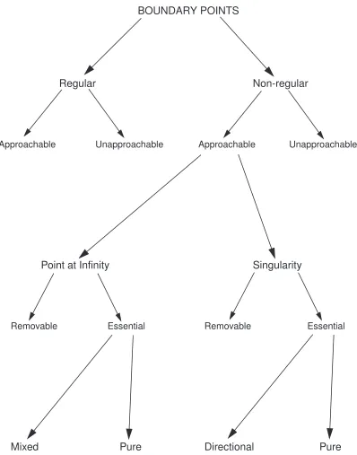
Figure 3.1, below, presents a schematic outline of the boundary point classification.
Regular points
3.1 The Abstract Boundary 31
3.1.27 Definition. Given a manifold M with a Ck pseudo-Riemannian metric g,
if there is an envelopment φ : M → Mφ so that there exists a Cl (1 ≤ l ≤ k)
pseudo-Riemannian metric gφ on Mφ, where gφ induces g, we shall say that φ is a
Cl extension, or that M
φ is aCl extension. Wherel =k we shall simply write that
φ is an extension.
3.1.28 Definition (Regular boundary point). A boundary point p of an envelop-mentφ :M → Mφ isCl regular for a metricg onM, if there exists a Cl extension
Mϕ with metric gϕ so that Mϕ ⊂ Mφ and φ|Mϕ =ϕ. Again, if l =k we drop the
Cl.
Points at infinity
Points at infinity are boundary points that are ‘far away’, with respect to the chosen family of curves. Points at infinity can be further subdivided into removable and essential points at infinity. In turn, essential points, at infinity can also be subdivided into mixed and pure points at infinity.
3.1.29 Definition (Point at infinity). Given a manifold M with a Ck metric g,
and a set C which satisfies the bounded parameter property, we shall say that a boundary point p of the envelopment φ : M → Mφ is a Cl point at infinity with
respect to C if,
1. the pointp is not aCl regular boundary point,
2. the pointp is a C-boundary point,
3. no curve in C approaches p with bounded parameter.
3.1.30 Definition (Removable point at infinity). A boundary point p which is a point at infinity is removable if there exists a boundary set B which covers p, so that for all x∈B,x is regular.
One can think of a removable point at infinity as a boundary point at infinity, that when re-expressed in a different envelopment becomes a set of regular boundary points.
Regular Non-regular
Approachable Unapproachable Approachable Unapproachable
Point at Infinity Singularity
Removable Essential
Mixed Pure Directional Pure
Removable Essential
[image:50.595.68.466.174.681.2]BOUNDARY POINTS
3.1 The Abstract Boundary 33
An essential point at infinity is a boundary point whose ‘far-awayness’ is a permanent feature of the space-time with respect to our class of curves C.
3.1.32 Theorem. Let p≡p0, then if p is an essential point at infinity so is p0.
Lastly, essential points at infinity can be subdivided into mixed and pure points at infinity. Mixed points at infinity have some character of regular points, where as pure points at infinity do not.
3.1.33 Definition (Mixed point at infinity). An essential point at infinity which covers a regular boundary point is a mixed point at infinity.
3.1.34 Definition (Pure point at infinity). An essential point at infinity which does not cover a regular boundary point is a pure point at infinity.
Singular points
We are now able to give the definition of a singularity. Just as for points at infinity, singular points can be subdivided into removable and essential singular points, and essential singular points can be divided again into directional and pure singular points.
3.1.35 Definition (Singular points). Let φ:M → Mφ be an envelopment with a
Ck metricg. A point p∈∂φM is a Cl singularity or is Cl singular if,
1. the pointp is not aCl regular boundary point,
2. the pointp is a C-boundary point,
3. there exists a curve inC which approachesp with bounded parameter.
3.1.36 Definition. A boundary set B is Cl non-singular if there does not exist an
x∈B so that x isCl singular.
3.1.37 Definition (Removable singularity). A Cl singular boundary point pis Cl
removable if it is covered by a Cl non-singular boundary set.
3.1.38 Definition (Essential singularity). A Cl singular boundary point p is Cl
essential if it is not Cl removable.