Scattering Theory

(1)

Scattering Theory

Sean Harris

October 2016

(2)

(3)

Declaration

The work in this thesis is my own except where otherwise stated. The first four chapters are largely expository, covering background material. The final two chapters contain mostly new theorems (to the best of my knowledge) proven by myself, with some help by others such as Professor Andrew Hassell.

(4)

(5)

Acknowledgements

Most of all I would like to thank my supervisor Professor Andrew Hassell, for developing my interest in this topic, always finding time to meet with me to discuss issues, and being generally great. I am also incredibly grateful to Dr Melissa Tacy for helping me draft this thesis while Andrew was absent. Thanks also goes to the many lecturers I have met leading up to this moment, for nourishing my interest in mathematics.

My fellow Dungeon-dwelling honours students have also been incredibly helpful throughout the year. Special mention to Hugh McCarthy, for always being available to chat about any problems I was having (both mathematical and otherwise).

A few more people to mention: my tutorial students, for giving me some reprieve from study; the staff at the ANU Food Co-op, for the great lunches (I wish I had discovered them earlier); and the many green envelopes and the single red envelope, for keeping me going.

I guess I should thank my parents too.

(6)

(7)

Abstract

Scattering theory studies the comparison between evolution obeying “free dynamics” and evolution obeying some “perturbed dynamics”. The asymptotic nature of free and perturbed evolution are compared to determine properties of the perturbation. A brief introduction to scattering theory and inverse scattering problems is given in Chapter3, after covering some relevant analysis concepts and the construction of Laplacian and Dirichlet to Neumann operators in Chapters 1 and 2. The spectral duality result of [EP95] is as follows.

Theorem ([EP95], Main Theorem). The following are equivalent:

1. −∆D has an M-fold degenerate eigenvalue k2₀

2. As k↑k0, exactly M eigenphasesθj(k) of SD(k) converge to π from below.

In Chapter4 this result is explained both mathematically and intuitively, and the significance of the form of the second equivalent statement is examined.

Possible generalisations of the main theorem of [EP95] to potential scattering are then inves-tigated in Chapter 5. The Cayley transform generalisation, as explained in Section 5.3, suggests studying an object which is given the name transmission operator. The transmission operator displays qualities similar to the scattering matrix and so is investigated further in Chapter 6. Many results about the spectrum of the transmission operator are proven under certain physically reasonable conditions on the considered potential for scattering.

(8)

(9)

Introduction

Our path to Scattering theory starts with the following problem:

Suppose we wish to determine properties of a person’s brain without intrusive testing. One possible way proceed would be to pass waves through the head, and observe the scattered waves which exit. We would like to know that this scattering information can return useful information, and so we will frame this as a mathematical problem.

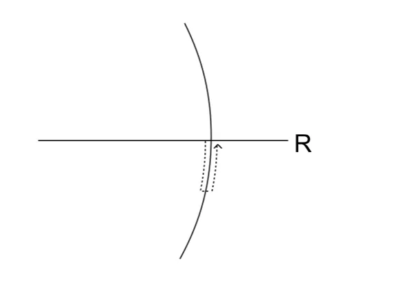
[image:9.595.164.451.489.707.2]

To find a starting point for such a theory, we may use the following thought experiment: Suppose you stand at the edge of a large lake inRn(this is mathematics, so the lake will of course be a ball). On top of this, suppose it is 2 a.m. and you are wearing your nicest shoes. In the middle of the lake, you can vaguely make out the shape of an object. Naturally you wish to determine properties of this object but you can’t see it very well due to the time of day, and you don’t want to ruin your shoes by swimming out to the object. All you can do is make splashes on the boundary of the lake, and measure the returning echoes (see Figure 1). From this wave scattering information, would it be possible to gain any knowledge of the object?

Figure 1: You stand on the edge of a lake and splash at the mysterious object. The grey solid line is the incoming and reflected wave, and the grey dotted line is the path the wave would have taken if there was no object.

(10)

The mathematical framework behind trying to solve such a problem is known as scattering theory. There are a few varieties of scattering theory, and the two we’ll focus on are potential and obstacle scattering, which both fall under the heading of concrete scattering theory. Potential scattering can be thought of as modelling waves passing through localised inhomogeneity in a media (such as a change of refractive index), while obstacle scattering can be thought of as modelling waves travelling through space with some forbidden region (such as electromagnetic waves travelling through a region with a conductive chunk of metal in the way).

Such a theory clearly has many real world applications, and it also has many interesting mathe-matical results! One such result is the spectral duality result of Eckmann and Pillet, given in their paper [EP95]. This spectral duality roughly states that an obstacle D appears “almost invisible” to some incoming radiation at frequencies approaching a given frequency k0, if and only if D can

support standing waves of the same frequencyk0.

The aim of this thesis is to explain the result of Eckmann and Pillet and to attempt to generalise the result to potential scattering. To do this, we shall start by covering some basic analysis facts, using [RS80] and [Are15] as main recource. These will be used to construct the Laplacian - a key component of scattering theory, and the Dirichlet to Neumann operators - a key component of our attempts to generalise the result of [EP95].

The Laplacian is a differential operator which governs the mathematical understanding of many physical processes. To us, its significance will be in passing from physical waves travelling through a lake to mathematical waves travelling through wherever the reader believes mathematics to live. The Dirichlet to Neumann operators relate the boundary values of some function satisfying certain physical laws on a domain, to the flux of said function through the boundary. These operators will be used to come up with a “local problem” to match the potential scattering problem, in the same way the standing wave problem matches the scattering off D.

After constructing these operators, we will explain how to pass from our physical problem of mystery objects in lakes and brain scans to a mathematical framework, known as scattering theory (following [Mel95]). This will leave us with enough knowledge to tackle the proof of Eckmann and Pillet’s, of which we will cover the main ideas.

(11)

Notation

H A separable Hilbert space over RorC.

ONB Orthonormal basis.

(·,·) An inner product on a given Hilbert space. If multiple Hilbert spaces are being considered, the inner product will be distinguished by subscripts. We use the convention that the inner product is conjugate linear in the second variable: (af, g) =a(f, g).

(·,·, . . . ,·) A tuple of elements from a given set.

V A a vector space overRorC.

|x| The standard Euclidean norm ofx∈Rn, or the norm of a numberx∈C. The distinction will be clear from the context.

||v|| The norm of a vector V in a Banach space. If multiple norms are considered, they will be distinguished by subscripts.

Γ(T) The graph of the linear operatorT.

D(T) The domain of the linear operatorT.

σ(T) The spectrum of the linear operatorT.

ρ(T) The resolvent set of the linear operatorT.

L(X),L(X, Y) The set of bounded linear transformtations from Banach spaceXto itself. The set of bounded linear transformations from Banach space X to Banach space

Y.

χΩ The characteristic function of the set Ω. I.e. for a set X containing Ω, χΩ :

X→_Ris the function which is identically 1 on Ω, and 0 elsewhere. ∆ The functional Laplacian, with sign convention based on Pn_i₌₁ _∂x∂

i.

∆U The Dirichlet Laplacian on U ⊂_Rn_{, with sign convention based on}Pn i=1

∂ ∂xi.

(14)

F The Fourier transform.

Λ, C A classical Dirichlet to Neumann operator and its Cayley transform, respec-tively.

Λ,C A semi-classical Dirichlet to Neumann operator and its Cayley transform, re-spectively.

SV(k), SD(k) The scattering matrix at frequencykfor potentialV or obstacleDwith Dirich-let boundary conditions, respectively.

H1(D), H2(D) Thep= 2 Sobolev spaces on D⊂Rn.

H₀1(D) The closure ofC_c∞(D) in H1(D).

(15)

Chapter 1

Background Analysis Concepts

This chapter will review some basics of the analysis techniques necessary throughout the rest of this thesis. These basics are more advanced than what is typically shown in an undergraduate degree in mathematics, but are still not the main component of this thesis so results will be given without proof. Most of the information below, and the relevant proofs, can be found in either [RS80] or [Are15]. Basic knowledge of Hilbert spaces and bounded operators will be assumed (roughly at an Analysis 3 level). However, the unfamiliar reader may find the earlier chapters of [RS80] a good reference for these concepts. Knowledge of Sobolev spaces will also be assumed. See [Eva10] for information. We will use the same notation as in [Eva10], which is repeated in Notation.

1.1 Unbounded Operators

There are many nice properties and definitions concerning bounded operators on Hilbert spaces, such as the notions of self-adjointness and compactness, and the spectral theorem for compact self-adjoint operators. However, in the real world bounded operators are incredibly limited. From a physics and PDE point of view, we would often like to know things about differential operators on function spaces. But differential operators are typically not bounded, as functions may have small norm, but vary wildly. This leads one to consider operators which are not required to be bounded. This section will discuss the main definitions and results for such operators.

First recall

Definition 1.1. A bounded operator on a Hilbert spaceH is a linear map T :H → H, such that there exists a constantC >0 with||T x|| ≤C||x||for allx∈X. The set of bounded operators on His written L(H).

This definition is too restrictive for our needs. We would still like some symmetry with respect to the inner product to be satisfied by the operators we consider. According to the Hellinger-Toeplitz Theorem (see Section III.5 of [RS80]), any operator T defined on all of H such that (T φ, ψ) = (φ, T ψ) for all φ, ψ ∈ H must necessarily be bounded. So we suppose that unbounded operators may not necessarily be defined on all of the Hilbert space we are working on, as is the case with differential operators on L2 spaces.

(16)

Definition 1.2. An operator A on H is a linear map from the domain of A, a linear subspace

D(A)⊂ H, toH.

Most of the operators we encounter will have dense domain, so this will be assumed unless specified otherwise. Such a general definition does lead to some issues with analysis, in that we know nothing about how the operator interacts with limits. So we make another definition, in an attempt to control limits.

Definition 1.3. Thegraph of an operatorT is the set

Γ(A) :={hφ, Aφi|φ∈D(A)} ⊂ H × H.

The product space H × H can be equipped with the inner product (hψ1, φ1i,hψ2, φ2i) := (ψ1, ψ2) + (φ1, φ2)

making H × Hinto a Hilbert space. A is called closedif Γ(A) is closed inH × H.

Note that the graph of an operator is a subspace of H × H, and we can always identify an operator with its graph. Depending on the domain which A is defined on, A may not be closed. However, if the domain is adjusted, it might be possible to define a closed operator extendingA.

Definition 1.4. LetA, A0 be operators onH. If Γ(A)⊂Γ(A0), then we sayA0 is anextensionof

A, and write A⊂A0. That is,D(A)⊂D(A0) and Aand A0 agree on D(A).

Definition 1.5. An operatorAis calledclosableif it has a closed extension. A closable operator

A has a smallest closed extension, which is denotedA.

One way to generate closed extensions of an operatorAis to take the closure of its graph, Γ(A). The issue with this is that the closure of the graph may no longer be the graph of an operator, that is it may contain points of the form h0, ψiforψ6= 0. However, ifA is closable, then it is easy to check that Γ(A) = Γ(A).

Definition 1.6. Let A be a densely defined operator on H. Let D(A∗) be the set of φ ∈ H for which there is an η∈ H with

(Aψ, φ) = (ψ, η) for all ψ∈D(A).

For eachφ∈D(A∗), we defineT∗φ=η as above. T∗ is called theadjoint of T.

It is clear that the adjoint as defined above is an operator, and that if A⊂B, then B∗ ⊂A∗. Note that if A did not have dense domain, then the above definition would not be well-defined (if D(A) is not dense, D(A)⊥ is non-trivial and we could add any element of D(A)⊥ to η while preserving the defining equality as above). In the case thatAis a bounded operator, this definition agrees with the usual definition of the adjoint constructed using the Riesz representation theorem. But in the case of unbounded operators, D(A∗) can be quite messy (even possibly just {0}!).

(17)

1.1. UNBOUNDED OPERATORS 3

Theorem 1.7 ([RS80], Theorem VIII.1). Let A be a densely defined operator onH. Then:

1. A∗ is closed.

2. A is closable if and only if D(A∗) is dense, in which case A=A∗∗. 3. IfA is closable, then (A)∗=A∗.

This theorem allows us to generally consider closable operators instead of their closures when considering things such as self-adjointness, which is typically very helpful in calculations.

Definition 1.8. LetA be a closed operator on H. A complex number λis in the resolvent set

of A, denoted ρ(A), if λI−A is a bijection ofD(A) onto H with bounded inverse. If λ∈ ρ(A),

Rλ(A) = (λI−A)−1 is called theresolventof A atλ

Theorem 1.9(First Resolvent Formula, [RS80], Theorem VI.5). Let Abe an operator onH. Then for λ, µ∈ρ(A), we have

Rλ(A)−Rµ(A) = (µ−λ)Rµ(A)Rλ(A).

The verification of this fact is a simple computation. There are a few other significant properties of the resolvent, which will be covered in the next section on differentiability and holomorphicity of Banach space valued functions.

Definition 1.10. Let A be a closed operator on H. The spectrum of A, denoted σ(A), is the compliment of ρ(A) in C. The spectrum is further divided into the point spectrum and the

residual spectrum. The point spectrum consists of all those λ for which there exists a non-zero φ ∈ D(A) such that Aφ = λφ, in which case λ is called an eigenvalue of A, with φ the correspondingeigenvector(sometimes called eigenfunction, eigenstate). The residual spectrum is everything in the spectrum that is not an eigenvalue.

We may sometimes refer to the spectrum of a closable, but not necessarily closed, operator, in which case we will always mean the spectrum of the closure.

Now we can define what it means for an operator to be self-adjoint. Note that this is a bit more complicated than in the bounded case, as we may have issues with domains. For this reason, we have an intermediate notion of a symmetric operator

Definition 1.11. A densely defined operator A on H is called symmetric ifA ⊂A∗. In other words

(Aψ, φ) = (ψ, Aφ) for all φ, ψ∈D(A).

Definition 1.12. A is called self adjointifA=A∗.

Note that by Theorem 1.7, A∗ is closed. So if A is symmetric then A ⊂A∗, so A∗ is a closed extension of A, so must also extendA=A∗∗. So for symmetric operators we have A⊂A∗∗ ⊂A∗, for closed symmetric operators we have A = A∗∗ ⊂ A∗, and for self adjoint operators we have

(18)

It turns out that this definition of self adjointness for unbounded operators is the correct one as these domain equalities allow one to form functional calculi, which we will see is incredibly important to scattering theory. It should be noted that actually checking an operator is self adjoint directly from the definition could be quite difficult. However, there are many nice theorems which give simple conditions to check self-adjointness, and to construct self adjoint extensions of symmetric operators. While these theorems give a wonderful classification of self adjoint extensions, they are not relevant to the material of this thesis. The interested reader should check [RS75].

As in the case of bounded self adjoint operators, it is easy to check that the spectrum of a self adjoint operator lies completely on the real axis. This will be important in the next section, when we define a functional calculus on self adjoint operators.

There are a slew of other definitions concerning operators, which give corresponding results on the spectrum. We say a self adjoint operator A is positive if (Ax, x) ≥ 0 for all x ∈ D(A), or that it is bounded below if there exists anM ∈_Rwith (Ax, x) ≥M||x||2_{. Note that a positive}

operator is bounded below with M = 0. We will use the notation A ≥ 0 to mean that A is a positive operator, and A≥B to mean A−B ≥ 0. Given A bounded below by M (or A≥ M I), it is quite easy to show that A−λI is invertible for any λ < M, and hence the spectrum ofA is bounded below by M. The proof of this is given as an exercise at the end of Chapter 8 of [RS80]. We will combine this knowledge with the following theorem and information about compact operators to obtain one of the most necessary theorems of this thesis, concerning self adjoint operators bounded below, with compact resolvent.

Theorem 1.13 (Hilbert-Schmidt Theorem, [RS80], Theorem VI.16). Let K be a compact self adjoint operator on H. Then there exists an ONB{φn} for Hso thatKφn=λnφn for eachn, and

λn∈R. If His infinite dimensional, then λn→0 as n→ ∞.

Recall also that the set of compact operators, denoted Com(H), form an ideal inL(H), that is Com(H) is a subspace ofL(H), and for any S, T ∈ L(H) andK ∈Com(H),SKT ∈Com(H). It is also common knowledge (amongst analysts) that Com(H) is norm closed and closed under taking adjoints. These properties are proven in [RS80].

Note that the first resolvent formula (Theorem 1.9) combined with these facts shows that if an operator A has compact resolvent Rλ(A) for some λ ∈ ρ(A), then Rµ(A) is compact for all

µ ∈ ρ(A). We can thus refer to operators with compact resolvent at some given point in their resolvent set as operators with compact resolvent.

These results can be combined to give the following desired theorem, concerning self adjoint operators, bounded below with compact resolvent.

Theorem 1.14. LetA be a self adjoint operator onHbounded below with compact resolvent. Then there exists an ONB {φn} for H consisting of eigenvectors of A with real eigenvalues {λn}. If H is infinite dimensional, then λn→ ∞ as n→ ∞.

(19)

1.2. DIFFERENTIABILITY AND HOLOMORPHICITY IN BANACH SPACES 5

1.13 is then applied to RM(A) to obtain an ONB{φn}for Hconsisting of eigenvectors of RM(A) with eigenvalues {µn}. It is then easy to check that eachφnis an eigenvalue of A, with eigenvalue

λn = M − _µ1_n. The convergence of eigenvalues is then proven by the analogous statement in Theorem1.13 and using the fact that Ais bounded below.

As one last result we include the following theorem, attributed to Riesz and Schauder, con-cerning compact operators not necessarily assumed to be self adjoint. This will play a major role throughout the later chapters of this thesis.

Theorem 1.15 (Riesz-Schauder Theorem, [RS80], Theorem VI.15). Let K be a compact operator on H. Then σ(K) is discrete, having no limit points except possibly at 0. Further, any non-zero

λ∈σ(K) is an eigenvalue of finite degeneracy.

1.2 Differentiability and Holomorphicity in Banach Spaces

There are many nuances to coming up with a definition of “differentiable” or “holomorphic” for Banach space valued functions. Differentiating operator valued functions and applying theorems of complex analysis will feature heavily in later chapters. Rather than giving a complete description of the different differentiability conditions, we will now give a very brief overview and some examples. For the most part, everything works as it does for complex valued functions.

For a Hilbert space valued function f :U ⊂ _R → H, the derivative is defined in the obvious way:

f0(t) = lim h→0

f(t+h)−f(t)

h .

It is easy to check that this notion of derivative satisfies the usual properties of a derivative, such as linearity and the following nice relationship with the inner product:

(f, g)0= (f, g0) + (f0, g).

The only Banach-space valued functions we will encounter will be operator valued. Typically these will have unbounded derivative, so we use the strong definition of the derivative. We say an operator valued function A on U ⊂ _R has derivative ˙A(t) at t ∈ U, an unbounded and densely defined operator onH, if for all v∈D

˙

A(t)

the following holds:

lim h→0

A(t+h)v−A(t)v

h = ˙A(t)v.

Example 1.16. For t ∈ [0,∞), let A(t) : R2 → L2([0,1]) be the operator sending the pair (a, b)∈_R2 _{to the solution of the following boundary value problem:}

( (−d2

dx2 −t2)u(x) = 0 on (0,1)

u(0) =a, u(1) =b.

Then at t0 ∈[0,∞), ˙A(t0) :R2 →L2([0,1]) sends the pair (a, b) to the solution of: (

(−d2

dx2 −t2₀) ˙u(x) = 2t0u(x) on (0,1)

˙

u(0) = 0, u˙(1) = 0.

(20)

We will also be confronted with situations in which understanding holomorphicity will be re-quired. For a Hilbert space valued function f from some open set U ⊂ _C to H, holomorphicity is defined exactly as one would expect. Namely, for each z ∈U the following limit is required to exist:

lim |h|→0

f(h+z)−f(z)

h .

Hilbert space valued holomorphic functions enjoy many of the properties of complex valued holo-morphic functions, such as local expressions as power series, infinite regularity and integral formulae. It is much more difficult to define a notion of holomorphic operator valued functions (also called a holomorphic family of operators). If we restrict to functions with image in the bounded operators, then we may say such functions are holomorphic if they admit local norm convergent power series representations.

Example 1.17. For an unbounded operatorT onH, the resolvent Rλ(T) is holomorphic. To see this, fix some λ0 ∈ρ(T). If we then consider λclose toλ0, we can find

Rλ0(T) I+

∞ X

n=1

(λ0−λ)n[Rλ0(T)]

n !

is a norm convergent power series for|λ−λ0|<||Rλ0(T)||

−1_{, and is the inverse of (}_λI₋_T_{). Hence}

ρ(T) is open, andRλ(T) is a holomorphic operator valued function. As a corollary, the spectrum of any operator is closed. This example was appropriated from Theorem VI.5 of [RS80].

Note that if A(z) is a holomorphic family of bounded operators in L(X, Y) for Banach spaces

X, Y, then for all x∈ X, y∗ ∈Y∗, both A(z)x and y∗(A(z)x) are holomorphic functions (Banach space valued and complex valued respectively). In fact, it can be shown that a family B(z) of bounded operators from X toY is holomorphic if and only if for allx ∈X the function B(z)x is holomorphic, if and only if for ally∗ ∈Y∗ the functiony∗(B(z)x) is holomorphic. This equivalence makes it much easier to check holomorphicity.

As mentioned at the beginning of Section 1.1, we will need to consider unbounded operators. The previous definition of holomorphicity clearly fails for unbounded operator valued functions so we will have to come up with a new one. This is done in [Kat95], Chapter 7. However, the constructions in [Kat95] are complicated and space consuming (over 60 pages!) so will be left to the reader to digest. Fortunately, every unbounded family of operators we will need to consider can be linked to a bounded family of operators via the spectral theorem of the next section, and so we may just bootleg the results from the bounded case.

1.3 The Spectral Theorem

In this section, we will outline the main results known as the Spectral Theorem. There are many different faces of the spectral theorem, and each is very powerful and relevant to the aims of this thesis.

The first form of the spectral theorem allows us to “take functions” of a self-adjoint operator

(21)

1.3. THE SPECTRAL THEOREM 7

basis {φi} given by eigenvectors of A, such that each φi has real eigenvalue λi. Then given any functionf :{λi} →C, we can define f(A) by settingf(A)φi =f(λi)φi and extending via linearity. We would like to apply this idea to the case that H is infinite dimensional, and the following theorem says that we can.

Theorem 1.18 (Spectral Theorem - Functional Calculus Form, [RS80], Theorem VIII.5). Let A

be a self adjoint operator on H. Then there exists a unique map φˆ from B(_R), the bounded Borel functions on R, toL(H) so that:

1. φˆ is an algebraic *-homomorphism, i.e.for all f, g∈ B(_R), λ∈_C, ˆ

φ(f g) = ˆφ(f) ˆφ(g) φˆ(λf) =λφˆ(f) ˆ

φ(1) =I φˆ(f) = ˆφ(f)∗.

2. ||φˆ(f)|| ≤ ||f||∞.

3. Suppose fn is a sequence of bounded Borel functions on R with hn(x) → x for each x ∈ R and |hn(x)| ≤ |x|for all x and n. Then for allψ∈D(A),φˆ(hn)ψ→Aψ.

4. Ifhn→h pointwise and ||hn||∞ is bounded, then φˆ(hn)→φˆ(h) strongly. 5. IfAψ=λψ, then φˆ(f)ψ=f(λ)ψ.

We will often write ˆφ(f) asf(A) in analogy with the construction in the finite dimensional case, and refer to ˆφ as a “functional calculus”. One of the most important applications of this form of the spectral theorem will be discussed in the later section on groups and semigroups.

There is an important point which is missed in the above theorem given the level of generality we have approached with. In the construction of the functional calculus for bounded operators, one can start with definingf(A) for continuous functionsf, defined only onσ(A). These are then used to extend the functional calculus to include all bounded Borel functions on R. But the functional calculus is still only “supported” on σ(A), in the sense thatf(A) =f◦χ_σ₍_A₎(A). This also holds for the unbounded self-adjoint operators A, although in that case this implicit dependence on only

σ(A) is hidden even deeper within the proofs. With this in mind, we have the following incredibly important theorem, a generalisation of property (v) in the previous theorem:

Theorem 1.19 (Spectral Mapping Theorem, [RS80], Theorem VII.1(e)). Let A be a self adjoint operator on H, and f be a bounded real valued Borel function on σ(A). Then σ(f ◦χ_σ₍_A₎(A)) is equal to the essential range of f, i.e.

{λ∈R;∀ >0, µ(m∈M;|f(m)−λ|< )>0}.

In the case f is continuous onσ(A), then σ(f ◦χσ(A)(A)) =f(σ(A)).

(22)

Theorem 1.20 (Spectral Theorem - Multiplication Operator Form, [RS80], Theorem VIII.4). Let

Abe a self adjoint operator onH. Then there exists a measure spacehM, µiwithµa finite measure, a unitary operator U :H →L2(M, dµ) and a real valued measurable functionf :M →_R which is finite µ-a.e. such that:

1. ψ∈D(A) if and only if f(·)(U ψ)(·)∈L2(M, dµ).

2. If φ∈U(D(A)), then (U AU−1φ)(m) =f(m)φ(m).

Remark 1.21. In applications, we will typically be able to find M and µ explicitly. In some instances, it will be more convenient to drop the finite assumption onµ, as we shall see in Chapter 2.

In the context of Theorem 1.20, the image off and the spectrum ofA can be directly related. Suppose for example thatf is identically equal toλ∈_Ron a measurable setB ⊂Mwithµ(B)6= 0. Then χB(m)6= 0 and (f(m)−λ)χB(m) = 0. We find:

A U−1χB

=U−1(f χB) =λU−1χB.

So Ahas eigenvalue λwith eigenvectorU−1χB 6= 0.

Now, suppose that λ is in the essential range of f (see Theorem 1.19 for the definition of essential range). Then for each n∈_N, choose a measurable set Bn⊂M of positive measure such that|f(m)−λ|< 1_n for allm∈Bn. Letφnbe the characteristic function ofBn, scaled to have unit

L2(M, µ) norm. Then it is easy to check that (f(m)−λ)φn→0 in L2(M, µ). By using continuity of U−1, it can be seen as before that (A−λI)U−1φn →0. But since ||U−1φn||=||φn||= 1, this implies that (A−λI) is not invertible, and soλ∈σ(A).

Before moving on to the last form of the spectral theorem, we need to use the previous theorem to specify some distinguished subsets ofσ(A). For a fixed self adjoint operator A, a vectorψ∈ H is said to be cyclic if {g(A)ψ|g ∈ C∞(R)} is dense in H (where C∞(R) is the set of continuous functions vanishing at infinity). The Riesz-Markov Theorem (see [RS75]) guarantees the existence of a Borel measure µψ on Rof finite mass, such that for all g∈C∞(R):

(ψ, g(A)ψ) = Z

R

g(λ)dµψ(λ).

The measureµψ is known as a spectral measure. In the case thatψ is cyclic forA, the spectral measure allows us to form a unitary map H → L2(R, dµψ), such that A is mapped to multi-plication by λ. In general, we can decompose H into a direct sum of (possibly infinitely many) subspaces such that each subspace has a cyclic vector, in which case we obtain a unitary map H → L∞_i₌₁L2(R, dµψi). For more information about this construction, see [RS75]. Now, for any

(23)

1.3. THE SPECTRAL THEOREM 9

Theorem 1.22 ([RS80], Theorem VII.4). Let A be a self adjoint operator on H. Let H_pp ={ψ∈ H |µψ is pure point}, Hac = {ψ ∈ H |µψ is absolutely cts} and Hs ={ψ ∈ H |µψ is singular cts}. Then H=Hpp⊕ Hac⊕ Hs, with each subspace invariant under A. A| Hpp has a complete basis of eigenvectors, A| H_pp has only absolutely continuous spectral measures and A| H_s has only singular continuous spectral measures.

From here we split the spectrum into distinguished subsets.

Definition 1.23.

σpp(A) ={λ|λis an eigenvalue ofA}, σcont(A) =σ(A|Hcont=Hac⊕ Hs),

σac(A) =σ(A|Hac),

σs(A) =σ(A|Hs).

Our definition used above is following the conventions used in [RS80]. Some authors use different notation, setting σpp(A) =σ(A| Hpp). With our conventions, we have the following theorem:

Theorem 1.24.

σcont(A) =σac(A)∪σs(A),

σ(A) =σpp(A)∪σcont(A).

This decomposition is incredibly important to scattering theory, which some mathematicians think of as the study of the absolutely continuous spectrum.

The final form of the Spectral Theorem which we will consider takes some more work to under-stand. First note that from the functional calculus form of the spectral theorem, for any measurable set Ω ⊂_R, we can form the operator PΩ = χΩ(A). Then due to the algebraic *-homomorphism

properties of the functional calculus, we find that:

1. Each PΩ is an orthogonal projection. That is,PΩ2 =PΩ∗ =PΩ.

2. P∅= 0, PR=I.

3. If Ω =F∞_n₌₁Ωn thenPΩ= s-limN→∞PN_n₌₁PΩn.

4. PΩ1PΩ2 =PΩ1∩Ω2.

A set of operators satisfying the above properties is called a projection-valued measure

(p.v.m). Note that for anyφ∈ H, (φ, PΩφ) is a well defined Borel measure onR, which is typically denoted byd(φ, Pλφ). We can then use the polarisation identity to defined(ψ, Pλφ) for allψ, φ∈ H. For a measurable Borel functiong:R→C, we can defineg(A) by setting

Dg ={φ| Z

R

(24)

and letting g(A) act on Dg via

(φ, g(A)φ) = Z

R

g(λ)d(φ, Pλφ),

using polarization to obtaing(A). We can write this symbolically as

g(A) = Z

R

g(λ)dPλ.

It is quite easy to check thatDg is dense inH, and that ifgis real valued theng(A) with domain

Dg is self adjoint. Note that we have thatA= R

RλdPλif{PΩ}is the family of spectral projections

related to A. This leads to the final form of the Spectral Theorem which we will consider.

Theorem 1.25 (Spectral Theorem - Projection Valued Measure Form, [RS80], Theorem VIII.6).

There is a one to one correspondence between self adjoint operators A and projection-valued mea-sures {PΩ} on H given by

A= Z

R

λdPλ.

If g is a real valued Borel function on R, then

g(A) = Z

R

g(λ)dPλ,

defined on Dg is self adjoint. If g is bounded, g(A) agrees with φˆ(g) of Theorem 1.18.

1.4 Forms

Working directly with operators can be quite difficult, and most operators occurring in physics tend to be obtained from something known as a form. Working with forms has many benefits over working with operators, making them typically the better choice for applications. We only need concern ourselves with bounded forms for the sake of this thesis, so will follow the material given in [Are15].

Definition 1.26. A sesquilinear form (or simply aform) on a vector spaceV overR (orC) is a map a: V ×V → R,(C), such that a is linear in the first variable and conjugate-linear in the second variable.

There are a few helpful properties of forms which we will need to cover. The form a is called

symmetricif for all u, v∈V

a(u, v) =a(v, u),

and accretiveif

<a(u, v)≥0.

If a form is accretive and symmetric, it will be called positive. We will also use the notation

(25)

1.5. GROUPS AND SEMIGROUPS 11

IfV is in fact a Hilbert space, we have some further definitions to give. We say the forma is

bounded if there exists someM ≥0 such that for all u, v∈V we have |a(u, v)| ≤M||u||_V||v||_V

and coercive if there exists someα >0 such that

<a(u)≥α||u||2_V.

With these definitions in hand, we can start to construct operators from forms.

Theorem 1.27 ([Are15], Propositions 5.5, 6.15, and Theorem 6.10). Let V,H be Hilbert spaces over R (C) and let a: V ×V → R(C) be a bounded form. Let j ∈ L(V, H) be an operator with dense range. Suppose further that if u∈V withj(u) = 0 anda(u) = 0, then u= 0. Then

A={(x, y)∈ H × H;∃u∈V :j(u) =x, a(u, v) = (y, j(v))∀v∈V}

defines an operator on H, called the operator associated to the pair(a, j)and denoted byA∼(a, j). Furthermore, ifj is compact thenA has compact resolvent, ifais symmetric thenA is self adjoint, and if ais positive then A is positive also.

This is quite a new way of obtaining operators from forms, and is quite powerful. There are many other useful properties ofAwhich are difficult to check, but can be determined directly from (much more easily verified) properties of aand the previous theorem. These are typically used for generating semigroups, and the interested reader may refer to [Are15] for more information.

Typically,jis an embedding ofV intoH, but particularly interesting operators can be obtained whenV and Hare very different spaces. We will see examples of both instances while constructing the Dirichlet Laplacian and Dirichlet to Neumann operators in Chapter2.

Note that ifais coercive, then the requirement in the preamble of Theorem1.27is guaranteed. Alternatively, if there exists some ω∈_R, α >0 such that

<a(u) +ω||j(u)||suchH2 ≥α||u||V2

for allu∈V, then we say thataisj-elliptic. Ifaisj-elliptic, then the requirement in the preamble is also readily verified.

1.5 Groups and Semigroups

Below is one form of the heat equation in one dimension,tas the time variable andx as the spatial variable

∂u ∂t =

∂2

∂x2u for all t >0

u(0, x) = g(x) for all x∈_R,

with initial conditiong in some function space onR. If we pretend that the operator A= ∂

2

∂x2 is a

constant, then we could form the symbolic solution

(26)

The basic motivation of semigroup theory is to make sense of the above expression, and use it to understand the dynamics of evolution equations.

Definition 1.28. Let X be a real or complex Banach space. A one-parameter semigroup on

X is a function T : [0,∞)→ L(X) satisfying

T(s+t) =T(s)T(t), for all t, s≥0.

If additionally

lim

t→0t(t)x=x, for all x∈X,

then T is called a C0-semigroup or a strongly continuous semigroup. If T is defined on R and the first property holds,T is aone-parameter group, and if the second condition also holds

T is called a C0-group

Example 1.29. The simplest example of a C0-group is the usual exponential. Given some fixed

a ∈ _R, we define T(t) on the Banach space R by T(t)x = eatx. It is easy to check that T is a

C0-group.

Example 1.30. As another simple example, letX be any Banach space, and fix someA∈ L(X). Define T(t) by

T(t) :=etA= ∞ X

j=0

(tA)j

j! .

It is easy to check that the sum above converges in norm (by using the triangle inequality, the fact that ||AB|| ≤ ||A|| ∗ ||B|| for all A, B ∈ L(X), and the convergence of the power series for the exponential onR). It is also quite easy to check that the defining properties of aC0-group are

satisfied by T(t). This example almost solves our issue with the heat equation mentioned at the beginning of this section, except that _∂x∂22 is unbounded (depending on its domain of definition)!

In the previous example, we say that etA is the semigroup generated by A. It turns out that allC0-semigroups have generators, in the following sense.

Definition 1.31. For a C0-semigroup T, we say A is the generator of T, whereA is the linear

operator with graph

A={(x, y)∈X×X|y= lim h→0+

T(h)x−x

h exists}.

There are some important properties of the generator of aC0-semigroup which we need to know

before being able to study them. These are collected below:

Theorem 1.32 ([Are15], Theorem 1.10). Let T be a C0-semigroup onX, with generatorA. Then

the following hold:

1. For x∈D(A), T(t)x∈D(A) for allt≥0, then function t7→T(t)x is continuously differen-tiable on [0,∞), and

d

(27)

1.5. GROUPS AND SEMIGROUPS 13

2. For allx∈X, t >0 one has Rt

0T(s)xds∈D(A), and

A

Z t

0

T(s)xds=T(t)x−x.

3. D(A) is dense in X, andA is a closed operator.

4. Lett0 >0, and letu: [0, t0)→X be continuous,u(t)∈D(A)for allt∈(0, t0),ucontinuously

differentiable on (0, t0), and u0(t) = Au(t) for all t ∈ (0, t0). Then u(t) = T(t)u(0) for all

t∈[0, t0).

5. LetS be a C0-semigroup on X, with generator B ⊃A. Then S=T, B =A.

It is the fourth property above that really relates semigroups to the solution of evolution equa-tions. Of course, we are much more interested in starting with an operator A, and then finding a

C0-semigroup so thatA is its generator, as this will then allow us to solve the evolution equation:

d

dtu(t) = Au(t) for allt >0

u(0) = g.

There is a large theory relating spectral properties of a given operatorAto whenAcan be used to generate a semigroup, and what properties the resulting semigroup achieves. However, only a very small part of this theory is relevant to the topics of this thesis. For a more elaborate view of semigroup generation, see [Are15].

What we will focus on is the generation ofC0-semigroups by self-adjoint operators on a Hilbert

spaceH. In this case, we actually want to construct the semigroupeitA_{, which will provide solutions} to the equation:

−i_dtdu(t) = Au(t)

u(0) = g.

This is then related to the wave equation: d2

dt2u(t) = −A2u(t)

u(0) = g.

So eitA is often considered a “wave operator”, where the above equation is a generalisation of the wave equation _dtd22u(x, t) = ∂

2

∂x2u(x, t). This is the basis of the “abstract” scattering theory, set

forth at the end of Chapter 3.

Since we are only interested in self adjoint operators, we can apply the spectral theorem in its functional calculus form (Theorem1.18) to defineeitA forAself-adjoint. This immediately implies the following properties:

Theorem 1.33. Let A be a self adjoint operator on H and defineU(t) =eitA. Then:

1. For each t∈_R,U(t) is a unitary operator (that is, (U(t)φ, U(t)ψ) = (φ, ψ) for allφ, ψ∈ H, or equivalently U(t)∗ =U(t)−1). Also, for alls, t∈R, U(s+t) =U(s)U(t).

(28)

3. For φ∈D(A), U(h)_hφ−φ →iAφ as h→0. 4. If limh→0U(h)φ−phi_h exists, then φ∈D(A).

We useU because the group is unitary, rather thanT, which is more commonly associated with translation. A family of unitary operators indexed byRsatisfying properties 1 and 2 above is called aC0- orstrongly continuous one-parameter unitary group. The following theorem of Stone’s

says that all strongly continuous one-parameter unitary groups are obtained by exponentiating iA

for some self adjoint operatorA.

Theorem 1.34(Stone’s Theorem, [RS80], Theorem VIII.8). LetU(t)be a strongly continuous one-parameter unitary group onH. Then, there is a self-adjoint operatorAonHsuch thatU(t) =eitA. The importance of unitarity should be made clear. The basic dynamics of quantum mechanics follow an equation of the form

−id

dtϕ(t) =Hϕ(t),

in which H is theHamiltonian, a self adjoint operator on a “state space”. Observable quantities in quantum mechanics are given by other self adjoint operators, A, in which an observation is formed by finding (ϕ(t), Aϕ(t)). Under certain commutation conditions onA and H (which I will not spell out, as commutativity is understandably complicated for unbounded operators, due to domain considerations), we can commuteA and U(t) to find

(ϕ(t), Aϕ(t)) = (U(t)ϕ(0), AU(t)ϕ(0)) = (U(t)ϕ(0), U(t)Aϕ(0)) = (ϕ(0), Aϕ(0)).

(29)

Chapter 2

The Laplacian and Dirichlet to

Neumann Operators

In this section, we will construct two of the most important operators in scattering theory, the Laplacian and the Dirichlet to Neumann operators, and determine some of their properties. We will (almost) only consider these operators on open subsets ofRn, but the definitions and theorems can be extended quite naturally to smooth manifolds.

2.1 The Laplacian

The Laplacian is a basic component of many PDE governing physical situations, such as the diffu-sion of heat and the propagation of waves.

The standard Laplacian on an open set U ⊂ Rn is defined to be the operator ∆ acting on a functionf ∈C2(U) as

∆f := n X

i=1

∂2 ∂x2

i

f.

We will take this sign convention. In this case −∆ will be a positive operator. This definition suffices forC2(U), and has many nice integration properties and relations to the Fourier transform (if U = Rn). But C2(U) is a difficult space to work over, especially when it comes to showing existence and uniqueness of solutions to PDE. So we need to come up with ways of extending the Laplacian to act on better spaces, ideallyL2(U). The good news is that this can be done, by using a the machinery already covered Chapter1.

To motivate our extensions, recall the following theorem:

Theorem 2.1 (Green’s Formula, [Eva10], Theorem 3 p.628). Let U ⊂ Rn be open with smooth boundary, u, v ∈ C2(U). Let dn and dS be the outward facing normal derivative operator and surface measure on ∂U respectively. Then:

1. R_UDu·Dvdx=−R

Uv∆udx+ R

∂UvdnudS

2. R

U(v∆u−u∆v)dx= R

(30)

If we take v compactly supported in U in the first formula, then Z

U

Du·Dvdx=− Z

U

v∆udx.

The left hand side of this looks like a form onH1(U), while the right hand side is an inner product of v with−∆u (up to taking the complex conjugate ofv). This suggests that we might be able to use our form methods to define a reasonable extension of the Laplacian toL2₍_U_{). Instead, we will}

start by extending to L2_loc(U). This brings us to our first extension of the Laplacian.

Definition 2.2. Thefunctional Laplacian∆ is defined as the operator onL2_loc(U) with domain

D(∆) = (

u∈H_loc1 (U);∃f ∈L2_loc(U) s.t. (Du, Dv) = (f, v),

∀v∈H1(U) compactly supported

)

defined by

∆u=−f.

This is the functional definition of the Laplacian, which only acts “locally”. It is easy to check thatH_loc2 (U)⊂D(∆), and for u∈H_loc2 (U), ∆u=Pn_i₌₁_∂x∂22

i

uin the weak sense. The domain of the Laplacian defined above is actually larger than H_loc2 (U) for certain U, although we will see later that ifU =Rn, thenD(∆)∩L2(Rn) =H2(Rn) exactly.

Definition2.2will suffice for defining Dirichlet to Neumann operators later in this chapter, but this definition does not have many nice properties beyond that. For the sake of Scattering Theory, we wish to be able to specify some kind of boundary conditions on solutions of PDE governed by a Laplacian-style operator. This is achieved by modifying the domain of the form considered above, and using our constructions relating forms and operators given in Section 1.4.

We will run through the construction of the Dirichlet Laplacian, ∆U, which has domain

D(∆U) ={u∈H01(U); ∆u∈L2(U)}. (2.1)

The Dirichlet Laplacian can be used to model the diffusion of heat or the propagation of waves when the dynamics are required to vanish on the boundary. Again, it is interesting to note that if the boundary of Dis not nice enough then it is possible to find elements of D(∆U) which are not in H2(U), although H2(U)∩H₀1(U) ⊂ D(∆U) always, with the same action as in the local case. To construct ∆U, we will consider the classical Dirichlet form,a:H01(U)×H01(U)→Cdefined by

a(u, v) = Z

U

Du·Dvdx.

Note thatais bounded, as

|a(u, v)| ≤ ||Du||_L2₍_U₎||Dv||_L2₍_U₎≤ ||u||_H1₍_U₎||v||_H1₍_U₎.

Now, if we let j:H₀1(U)→L2(U) be the usual inclusion, we find that

(31)

2.1. THE LAPLACIAN 17

So ais j-elliptic. Hence we can form the operatorA associated to (a, j), using Theorem 1.27. We claim (and it is easy to verify), that A = −∆_U as defined in Equation 2.1. For a more detailed explanation of this construction, see Example 5.13 of [Are15]. Note−∆U is positive and self adjoint by Theorem 1.27, sinceais positive and symmetric, and so has spectrum lying in [0,∞).

In the case that U is bounded with continuous boundary, the Rellich-Kondrachov Theorem (Theorem 7.11 of [Are15]) states thatjis compact, in which case Theorem1.27states that−∆Uhas compact resolvent. So L2(U) has an ONB consisting of eigenvectors of −∆_U with real eigenvalues, due to Theorem1.14, and these eigenvalues must be real, discrete and converging to +∞. This will be an incredibly important property when we consider Concrete Scattering Theory in Chapter 3. A similar construction can be used to show that forV ∈L∞(U) real valued, the operator−∆_U+V

is self adjoint, bounded below, with compact resolvent and so L2(U) has an ONB consisting of eigenvectors of−∆_U+V with real eigenvalues, which are discrete and converge to +∞(see [Are15] for details).

For an open setU ⊂_Rn_{, we call the equation}

(−∆−k2)u= 0 on U (2.2)

the Helmholtz equation at frequency k, or energyk2, onU. Note that this uses the functional Laplacian, so there are no assumed boundary conditions. For example, ifU =Rn, we obtain for each

θ∈Sn−1 a solution Φ0(k, x, θ) =eikx·θ of the Helmholtz equation at frequencyk. These solutions

do not lie in any reasonable Lp space besides L∞. There are many local regularity theorems concerning solutions of the Helmholtz equation, although as this example shows global regularity is not guaranteed. In this way, the Helmholtz equation doesn’t necessarily give eigenfunctions of the Laplacian on a sensible space. However, these solutions are incredibly important to scattering theory, as we shall see in Chapter 3.

2.1.1 The Laplacian in Spherical Coordinates

Throughout some of the calculations performed in later chapters we will wish to use some spherical symmetry arguments, decomposing functions into a certain collection of functions called spherical harmonics. This will allow us to perform calculations on the spherical harmonic decomposition, in which symmetry arguments are best suited. For this purpose, we will introduce the spherical Laplacian. It will become apparent that this operator will only be applied to sufficiently smooth functions, and so can just be given in terms of an explicit formula rather than as an unbounded operator with specified domain.

Given a functionf(x)∈C2(U) on some open set U ⊂Rn with continuous boundary, we may pass to spherical coordinates r =|x| ∈ [0,∞), θ = _|x|x ∈Sn−1, in which case we may consider f as a function from some subset of [0,∞)×Sn−1 _to

Cgiven byf(r, θ) =f(rθ), wheneverrθ∈U. The standard Laplacian on U can then be expressed in these new coordinates, with the formula:

∆f(r, θ) = ∂

2

∂r2f(r, θ) +

n−1

r ∂

∂rf(r, θ) +

1

(32)

where ∆tan is the tangential Laplacian acting on C2(Sn−1), andSn−1 is given its usual smooth

structure induced by its inclusion into Rn. For information about this, see any text on differential geometry, such as [Can13]. In the casen= 2, the tangential Laplacian onS1 is given by ∆tang(θ) =

∂2

∂θ2g(θ), and in higher dimensions there is a more complicated formula which is still known explicitly.

As in our extension of the Laplacian to L2, the tangential Laplacian onSn−1 may be extended to an unbounded self adjoint operator onL2₍_Sn−1_{). In this case the self adjoint extension is unique,}

because there are no boundary conditions which can be changed (since Sn−1 has no boundary). For a construction of this extension, see Section 7 of [Can13]. We will need some properties of this self adjoint extension:

Theorem 2.3 (Sturm-Liouville Decomposition, [Can13], Theorem 44). There exists an ONB {Θi(θ)} of L2(Sn−1) consisting of eigenfunctions of ∆tan, with eigenvalues {Ci}, such that:

0≤C1 ≤C2 ≤. . .

Furthermore, Θi ∈C∞(Sn−1) for each i.

The functions Θi are referred to asspherical harmonics. This theorem holds in more gener-ality, replacing Sn−1 with any compact smooth Riemannian manifold. The proof given in [Can13] is very nice, and works by considering diffusion under a heat equation. In keeping with our sign convention for the Laplacian onRn, the tangential Laplacian on the sphere has non-positive eigen-values. For this reason, some consider the Laplacian to be−∆tan.

Now we may finally get to the main purpose of this section, the decomposition of a function into spherical harmonics.

Theorem 2.4. GivenU ⊂Rn open bounded and symmetric about the origin, and somef ∈L2(U), there exists functions Ri from an open bounded subset of [0,∞) to C, such that:

f(r, θ) = ∞ X

i=1

Ri(r)Θi(θ),

in the L2(U) sense. Iff is smooth, each Ri is smooth.

Proof. To begin the proof, recall the fact that given two measure spaces (M, µ) and (M0, µ0), and ONBs{φi(x)}forL2(M, µ),{ψi(y)}forL2(M, µ), then{φi(x)ψj(y)}is an ONB forL2(M×M0, µ⊗

µ0). This is proven on page 51 of [RS80].

Since U is spherically symmetric around the origin, we may writeU =I×Sn−1 for some open bounded set I ⊂ [0,∞), where r ∈ I and θ ∈ Sn−1. There is some issue with this identification if 0 ∈ I. However, note that for the measure on I ×Sn−1 _{to be the Lebesgue measure (up to}

identification of f(r, θ) = f(rθ)), the measure on I must be rn−1dr (this is common knowledge, and can be found in any vector calculus textbook). Then {0} ⊂ _R2 _{has measure zero, as does}

{0} ×Sn−1 ⊂I×Sn−1, so both subsets can be ignored in considering L2 spaces.

(33)

2.2. THE SPECTRAL THEOREM APPLIED TO ∆ 19

Hence we can represent:

f(r, θ) = ∞ X

i,j=1

aijψj(r)Θi(θ) = ∞ X

i=1

Ri(r)Θi(θ),

whereRi(r) =P∞_j₌₁aijψj(r). Since the sum representingf(r, θ) converges inL2 and{ψj(r)Θi(θ)} is an ONB, the sum P∞_i,j₌₁|aij|2 must converge, and hence Ri ∈L2(I, rn−1dr). Note by orthonor-mality of {Θi(θ)}, we find

Ri(r) = (f(r, θ),Θi(θ))_L2₍_Sn−1₎.

If f is smooth f will be smooth in the r variable, and hence we can differentiate the above in r

(passing through the integration in the inner product, since everything is well behaved), to find that Ri(r) is smooth.

The main use of this theorem is the justification of separation of variables, used as a method of solving PDE with spherical symmetry. We will see many examples of this in Chapter 6. This actually requires more work, as we would like to differentiate term by term. In general, if a series of functions converges in L2 the such term-wise differentiation is not valid, so we need improved our method of convergence. Ideally we would like uniform convergence, at least locally. That uniform convergence holds is quite difficult to verify, and will generally require specifying the type of PDE the given function must satisfy, and using regularity and uniqueness arguments. Luckily for us, this has been checked in [Gus99] and will hold in each case investigated in this thesis.

2.2 The Spectral Theorem applied to

∆

Throughout this section we will work with ∆_Rn, which is self-adjoint as shown in Section 2.1. So

we can use the spectral theorem in the multiplication operator form, Theorem1.20applied to ∆_Rn.

This provides a measure space (M, µ), a unitary operator U : L2(Rn) → L2(M, dµ) and a real valued function f :M →_R which is finiteµ-a.e. such that:

1. u∈D(∆_Rn) if and only iff(·)(U u)(·)∈L2(M, dµ).

2. If φ∈U(D(∆_Rn)), then (U∆ RnU

−1_φ₎₍_m_{) =}_f₍_m₎_φ₍_m₎

In this case, we can give (M, µ) andU explicitly. In fact, we can take (M, µ) to beRnwith Lebesgue measure and U to be the Fourier transform.

Theorem 2.5([RS75], Theorem XI.6 and unnumbered Lemma on page 2). The Fourier transform F :L2(Rn)→L2(Rn) given by

F(u)(ξ) = 1 (2π)n2

Z

Rn

f(x)e−ix·ξdx

(34)

Sincef(ξ) =−|ξ|2_{is not constant on any sets of positive measure, the remark following Theorem}

1.20 implies that ∆_Rn has no eigenvalues. In fact, since f is continuous ∆

Rn has only purely

absolutely continuous spectrum, equal to Ranf = [0,∞).

Note that the properties given by Theorem 2.5 work for the functional Laplacian ∆ (although the functional Laplacian is not self adjoint) as for ∆_Rn whenever the Fourier transform of something

inD(∆) can be defined. We also have the familiar result:

Theorem 2.6 ([RS75], unnumbered Lemma, page 2). Foru∈H1(Rn) andj ∈ {1, . . . , n}

F(−i ∂ ∂xj

f)(ξ) =ξjF(f)(ξ).

These properties of the Fourier transform are incredibly useful for solving PDE and analysing systems. For our purposes, the Fourier transform is very important in Concrete Scattering Theory, as covered in Chapter 3.

We will now prove a useful result using the Fourier transform. Note that it is clear from the definition of the functional and Dirichlet Laplacians on Rn thatD(∆)∩L2(Rn) =D(∆Rn). So as

promised after Definition 2.2, we shall prove the following theorem:

Theorem 2.7. D(∆_Rn) =H2(_Rn)

Proof. Showing thatH2(Rn)⊂D(∆Rn) is trivial. So suppose thatu∈D(∆Rn). By Theorems2.5

and 1.20,|ξ|2_(F_u₎₍_ξ₎_∈_L2₍

Rn). But then for each i, j= 1, . . . , n: |ξiξj(Fu)(ξ)| ≤ |ξ|2|(Fu)(ξ)| ∈L2(Rn)

So ξiξj(Fu)(ξ) ∈L2(Rn). Taking the inverse Fourier transform and applying Theorem 2.6 shows ∂

∂xi

∂

∂xju(x)∈L 2₍

Rn). Since this holds for all i, j= 1, . . . , n, we find u∈H2(Rn) as claimed.

2.3 Dirichlet to Neumann Operators

Dirichlet to Neumann type operators are incredibly important in applications, so this section will start by motivating their study.

Suppose you have some open set U in Rn with some density function ρ on U. Think of U as your own head, and ρ as mass density function. Say that you would like to know the value of ρ

to determine properties of your head, such as possible medical issues. Ideally you would like to determine properties ofρ without any intrusive measurements of U, so only measurements on∂U

can be made.

(35)

2.3. DIRICHLET TO NEUMANN OPERATORS 21

(

Lu = 0 on U

u ≡ f on ∂U, (2.4)

for some second order differential operatorLdepending onρ. So, up to some rescaling, Λf =dnu, where f, u are as above, and dn is the outward facing normal. Would knowing Λ be enough to reconstruct ρ?

This clearly has many practical purposes, from medical imaging to determining conductivity of a medium to geology. The problem was first posed by Albert Calder´on (see [Cal80]).

We will consider a special case of this, in which L = −∆ +A, for some real-valued bounded measurable functionAonU. This has significant applications in attempting to generalise the results of [EP95] to potential scattering with potential A, as we shall see in Chapter 5. In some sense, the Dirichlet to Neumann operator produces reasonable “inside problems” for potential scattering, in analogue to the inside problem of the main result of [EP95], the Dirichlet eigenvalue problem. Before showing that a Dirichlet to Neumann style operator exists for suchL we need to generalise the definition of normal derivatives, since solutions of Equation 2.4 withf not smooth will fail to be smooth. The main aim is that an analogue of Green’s Formula (Theorem2.1) holds. So we have the following definition:

Definition 2.8 (Weak Normal Derivative, [Are15], Section 7.3). LetU ⊂Rn be bounded withC1 boundary. Let u∈H1(U) with ∆u∈L2(U). We say u has (outward pointing) weak normal derivativednu∈L2(∂U) if there exists an h∈L2(∂U such that for allv∈H1(U)

Z

U

Du·Dvdx+ Z

U

v∆u= Z

∂U

vhdS,

In which case we write dnu=h.

Note that if u ∈ C2₍_U_{) then the above definition agrees with the standard notion of normal}

derivative. So by using the density ofC2(U) inH1(U), it can be shown that weak normal derivatives are unique, when they exist. Interestingly, we can define the class of functions with “dnu= 0” for

U open with arbitrarily complicated boundary, as the set of u ∈ H1(U) with ∆u ∈ L2(U) such that for all v∈H1(U)

Z

U

Du·Dvdx+ Z

U

v∆u= 0.

In this sense, the weak normal derivative is much nicer than the standard normal derivative of second year calculus.

2.3.1 Dirichlet to Neumann Operator with respect to −∆

Now we will construct the Dirichlet to Neumann operator Λ0 forL=−∆ on an open bounded set

U ⊂_Rn_with_C1_{boundary, and determine some of its properties. This will again use the machinery}

of quadratic forms explained in Chapter 1, but will use the full force of Theorem 1.27 with j not just an inclusion.

The operator we are aiming for has graph

(36)

Before we get to constructing such an operator, recall the following:

Theorem 2.9 ([Are15], a conglomeration of many theorems and remarks from Chapter 7). Let

U ⊂ _Rn _{be open and bounded with} _C1 _{boundary. There exists a unique bounded operator tr} _:

H1₍_U₎ _→ _L2₍_∂U₎ _{known as the} _{trace operator}_{, such that tr(}_u_{) =} _u_|

∂U for all smooth u. The trace operator is compact.

We will typically write tr(u) =u|∂U. We will also extend the classical Dirichlet form

a(u, v) = Z

U

Du·Dvdx

to the domainH1(U)×H1(U). We will construct Λ0 as the operator associated with (a,tr) using

Theorem1.27, after the following Lemma.

Lemma 2.10 ([Are15], Proposition 8.1). The form a as above is tr-elliptic. Now we come to our existence theorem:

Theorem 2.11 ([Are15], Theorem 8.4). The operator A on L2(∂U) associated to(a,tr) via The-orem 1.27 agrees with the desired Dirichlet to Neumann operator Λ0; that is

Γ(A) ={(f, g)∈L2(∂U)×L2(∂U);∃u∈H1(U),−∆u= 0, u|∂U =f, dnu=g}. The operator Λ0 is self-adjoint and positive, with compact resolvent.

Remark 2.12. Applying Theorem1.14shows thatL2(∂U) has an ONB consisting of eigenvectors of Λ0, each having positive eigenvalue and such that the eigenvalues converge to +∞.

2.3.2 Dirichlet to Neumann Operator with respect to −∆ +A

While the Dirichlet to Neumann operator with respect to−∆ is quite interesting, it is far from good enough for the purposes of the rest of this thesis. To be able to generalise the main result of [EP95] to potential scattering, we need to come up with an “inside problem” for potential scattering. For this, we would like to consider ΛA, the Dirichlet to Neumann operator with respect to the operator

L=−∆ +A, whereA∈L∞(U) andAonly takes real values. Such anLcan be used for modelling the motion of waves or diffusion of heat through an inhomogeneous medium.

One issue in this case is that uniqueness of solutions to (

Lu = 0 onU u ≡ f on∂U

are no longer guaranteed (as they are in the case L=−∆). For example, if 0∈σ(−∆_U +A),

then we can add anyu0 ∈ker(−∆U +A) to u as above to find (

(37)

2.3. DIRICHLET TO NEUMANN OPERATORS 23

since u0 ∈ H₀1(U). But then we might find that dnu 6= dn(u+u0), so the Dirichlet to Neumann operator can’t be defined uniquely (although it will still be a linear relation).

Luckily we have the following theorem, courtesy of [Are15].

Theorem 2.13 ([Are15], Theorem 8.14). Suppose 0∈/σ(−∆U+A). Then

{(f, g)∈L2(∂U)×L2(∂U);∃u∈H1(U),−∆u+Au= 0, u|∂U =f, dnu=g}

is the graph of a a self-adjoint operator ΛA with compact resolvent. Also, ΛA is bounded below. The proof of this theorem requires a lot of supplementary results, so will not be given. The interested reader may find the proof in [Are15] however.

(38)

(39)

Chapter 3

Scattering Theory

In this chapter we will introduce Scattering Theory in two main flavours: concrete and abstract. The focus will be on concrete scattering theory, as this is most relevant to our objectives. However, the abstract formulation has some important qualities, so will be briefly mentioned at the end.

We will start by setting up the mathematical framework behind the real world problem given in the Introduction, which will be referred to as Concrete Scattering Theory. As a basic case, we will start by looking at trivial scattering in which there is no object.

3.1 Trivial Scattering

Given we wish to examine asymptotics of waves, we will start by examining solutions to the wave equation:

−∆u(x, t) =−∂

2

∂t2u(x, t), onR

n_×

R. (3.1)

As discussed in Section2.2, the spectrum of −∆_Rn is positive and is purely absolutely continuous.

So −∆ has no eigenfunctions inL2 (notingD(∆)∩L2(Rn) =D(∆Rn)). However, we may consider generalized eigenfunctions of −∆ on _Rn_{, that is, bounded solutions of}

−∆u(x) =k2u(x),

where we take k real and greater than 0, since −∆_Rn has positive spectrum. Then eiktu(x) will

be a bounded solution of Equation 3.1. We exclude the case k = 0, as this corresponds to no evolution in time. So instead of the time dependent equation 3.1, we will look at the generalised eigenfunction time independentequation, which is

(−∆−k2)u(x) = 0, on Rn, (3.2)

fork >0. This is the Helmholtz equation, as described in Section2.1. As our physical problem re-quires examining asymptotics of solutions of the Helmholtz equation, we also impose theradiation conditions:

∂ ∂r+ik

2

u(rθ)∈L2(Rn). (3.3)

(40)

where r=|x|, θ = _|x|x are the spherical coordinates. We will call solutions of any of the PDE that we encounter which satisfy these radiation conditionsscattering solutions.

The keen reader might have noticed that the plane waves Φ0(k, x, θ) :=eikx·θforθ∈Sn−1satisfy

these two conditions. Essentially, the radiation condition is required to remove the possibility of the plane waves e−ikx·θ, which will be used for uniqueness results later. We can use this to obtain a wide class of solutions in the following way. Giveng∈C∞(Sn−1), we define the functionH0(k)g

on Rnby:

(H0(k)g)(x) =

Z

Sn−1

Φ0(k, x, ω)g(ω)dω.

Checking that H0(k)g satisfies Equations 3.2 and 3.3 and that it is bounded is trivial, by

commuting integration and differentiation (valid since everything is smooth and integration is over a compact set) and using the fact that Φ0(k, x, θ) satisfy the same equations.

Now we may apply the Principle of Stationary Phase to obtain an asymptotic form for H0g,

expressed in spherical coordinates r=|r|,θ= _|x|x:

H0(k)g)(rθ) =

eikr

(kr)12(n−1)

e−14π(n−1)ig(θ)

+ e

−ikr

(kr)12(n−1)

e14π(n−1)ig0(θ) +O(r− 1

2(n+1)), asr → ∞

The Principle of Stationary Phase essentially says that since we are integrating against a highly oscillatory function Φ0(k, x, ω), the main contributions to the integral come from the points where

the phase x·ω is stationary in ω, which is at ω = ±θ. See [Ros03] for more information. A consequence of applying this is that

g0(θ) =in−1g(−θ)

To interpret this asymptotic form in the terms of our original problem, we can reintroduce the time dependence, obtaining the travelling wave:

eik(t+r)

(kr)12(n−1)

e−14π(n−1)ig(θ) + e

ik(t−r)

(kr)12(n−1)

e14π(n−1)iin−1g(−θ) +O(r− 1

2(n+1)) (3.4)

The first term will maintain constant phaseeik(t+r) along curves of withr+t, so astincreasesr

must decrease, representing an incoming wave. Similarly, the second term will have constant phase

eik(t−r) along curves of constant t−r, and so represents an outgoing wave. The factors r−12(n−1)

cause dissipative nature asr increases. This form provides one lemma, which we require before we can relate this solution to our scattering problem. This lemma provides us with uniqueness of the associationg7→g0.

Lemma 3.1 ([Mel95], Lemma 1.2). For each k > 0 and g ∈ C∞(Sn−1) there exists a unique scattering solution u of Equations3.2 of the form

u= e ikr

r12(n−1)

g(θ) + e −ikr

r12(n−1)

g0(θ) +O(r−12(n+1)), as r → ∞.

Scattering Theory

Scattering Theory

Sean Harris

October 2016

Declaration

Acknowledgements

Abstract

Introduction

Contents

Notation

Chapter 1

Background Analysis Concepts

1.1

Unbounded Operators

1.2

Differentiability and Holomorphicity in Banach Spaces

1.3

The Spectral Theorem

1.4

Forms

1.5

Groups and Semigroups

Chapter 2

The Laplacian and Dirichlet to

Neumann Operators

2.1

The Laplacian

2.2

The Spectral Theorem applied to

∆

2.3

Dirichlet to Neumann Operators

Chapter 3

Scattering Theory

3.1

Trivial Scattering