A Novel Approach on Power System Fault Detection Using Bayes Optimisation

International Journal of Innovative Technology and Exploring Engineering (IJITEE) ISSN: 2278-3075,Volume-8 Issue-6, April 2019



Abstract. One of the substantial tools for the diagnosis of the transmission line faults is the artificial neural network, due to its ability to distinguish between variegated configurations. The data fed to the network get noisy sometimes that cause miscalculate at the output of the plant. By using Bayesian optimization techniques which commission the naive baye’sprocess [11] that minimize the sample data to quench the misreading at the output. “This process scrutinizes the use of an optimization technique to pinout the selective collection of data set in real time using limited amount of sample data. Importantly, this paper investigates with the Bayesian approach that mixes the strengths of bayesian optimization [13]. The usage of gaussian regression strategies [15] requires just a few number of information factors to model the complex goal gadget. Moreover because of using trust place constraint on sampling process, bayesian analysis tends to growth the target cost and converge toward near the superior. Simulation research the use of analytical features display that the Bayesian optimization can achieve an almost optimizing in a target value with rapid convergence. And these converged data sets are used to rehearse artificial neural networks (ANNs) for the fault classification in” high voltage transmission lines. The back propagation algorithm [19] and gradient boosting function has been employed for detection and classification of the fault type.

Keywords: power system faults, neural networks, optimization.

I.INTRODUCTION

The electric utilities organizations are required to give buyers a persistent and fantastic administration at a focused and sensible expense. This implies they need to safeguard the unwavering quality of the framework to give shoppers an administration what is “predictable with the security work force and hardware, and satisfy their needs inside indicated voltage and recurrence. Blames in the transmission lines are one of the components that the unwavering quality of the framework is influenced by. The more blames that happen, the less dependable the framework is, since they could cause blackouts in the power framework, which may result in an intrusion of the administration. In this manner, when planning the power transmission frameworks, electric organizations are required to pursue the arrangement of standard determinations, the less blames events will be and the more solid the power framework will” be. To diminish the shortcomings and impact of flaws, compels identified with the transmission framework get the chance to improve. Enhancement is the scientific strategy which is worry with

Revised Manuscript Received on April 07, 2019.

V Vijay Kumar, Department of EEE, Godavari Institute of Engineering and Technology (A), Rajahmundry, India,

Jillella Gopinath, Department of EEE, Godavari Institute of Engineering and Technology (A), Rajahmundry, India

finding the most extreme and least of the capacity, perhaps subject to the requirements for nonstop and differential capacities. Enhancement approach can be utilized in various regions like engineering, financial aspects, material structure and transportation yet in this paper we center around voltage mutilations in three stage organize because of issues and characterize the sort of blame utilizing neural system by streamline the system parameters utilizing baye's hypothesis. “The idea of bayes' hypothesis is one of the major and critical speculations among contingent likelihood. As per the likelihood hypothesis, the contingent likelihood can decide bycalculating the likelihood of an activity happened at a given another occasion has happened. On the off chance that the some occasion An and occasion B are expected to have happened then the contingent likelihood of A given upon B or the restrictive likelihood of B given upon An is typically composed as P(A|B). For instance, the likelihood that any given transmission line has a blame on some random unit of time might be x%. In any case, on the off chance that we know or expect that the line which get blame condition, at that point they are substantially more prone to be glitch of hardware now and then harm. The contingent likelihood of hardware harm given that you have a blame on framework may be an a lot higher X%.” This procedure is determined by utilizing baye's hypothesis [11] that gives estimated likelihood esteem utilizing typical conveyance which the given information is have a place with either flawed esteem or non-defective esteem. So by utilizing probabilistic capacity P(A|B), we can arrange the informational collections that we gauged amid blame happened on three stage line and limit the mistake at the characterization organize [4]. “The way toward perceiving the kind of blame is finished by a neural system prepared by the information which experiences through the streamlining. The procedure is essentially looks a ton due to the extensive number of informational indexes get handled in disconnected condition. Yet, the outcome toward the end is very fulfilled when contrasted and the non-advanced information that yields colossal blunders on account of rehashed estimations and commotion amid the task of three stage transmission framework”.

II. FAULT CLASSIFICATION ON POWER SYSTEM Deficiencies can be characterized as the stream of a high plentifulness current throughan ill-advised way which could cause substantial equipmentdamage which will prompt interference of intensity, individual damage.

A Novel Approach on Power System Fault

Detection Using Bayes Optimisation

In augmentation, the size of voltage level will alternatewhich can influence the hardware protection in the event of anincrease or could cause a disappointment of gear start-up if thevoltage is beneath a base dimension [1]. “Hence,equipment will be presented to the threat ofelectricity which isn't accepted.In request to forestall suchan occasion, control framework blame investigation was presented. Theprocess of assessing the framework voltages and flows under different kinds of hardware conditions is called blame examination [3], whichcan decide the important security measures and the requiredprotection framework. It is fundamental to ensure the security of open .The examination of shortcomings prompts appropriateprotection settings which can be figured so as to selectsuitable wire, electrical switch size and kind of hand-off. Theseverity of the blame relies upon the short or open circuit areas, thepath taken by blame current, the framework impedance and itsvoltage level. So as to keep up the continuation of intensity supply to all clients which is the center motivation behind the power framework presence, all blamed parts must be segregated from thesystem transitory by the security plans.” At the point when a blame exists inside the assurance zone at any transmissionline, a flag will excursion or open the electrical switch secluding thefaultedline.Faults as a rule happen in a power framework because of protection breakdown, flashover, and physical harm. Thesefaults may either be three stages in nature including all threephases in a symmetrical way, or might be asymmetricalwhere normally just a single or two stages might be included. Faultsmay likewise be brought about by either shortcircuits to earth or betweenlive conductors, or might be brought about by broken conductors inone or more stages. Now and then concurrent deficiencies may occurinvolving both short out and broken-conductor blames otherwise called open-circuit faults.Overhead transmission line presented to basic climatic conditions, so the odds ofoccurrence of issues in overhead transmission lines were more when contrasted with underground links. Faultsin overhead transmission framework can be arranged into two kinds, for example open circuit blames and short out blame. Open circuit deficiencies can be recognized effectively by watching the each stage voltage. In the event that the voltagevalues expands, it shows that open conductor blame is happened. “These shortcomings are very rarelyoccurredfaults.Short circuit issues can be distinguished effectively by watching the each stage current. In the event that the present qualities increases,it shows cut off is happened. Short out issues are partitioned into two sorts, for example asymmetricalfaults, and symmetrical issues [2] [3]. Uneven shortcomings line to ground, line to line, and twofold line to ground, and symmetrical deficiencies are triple lineand triple line to ground issues. A vital target of all the power frameworks is to keep up an abnormal state of continuityof administration, and when unusual conditions happen, to limit the blackout times. It ispractically difficult to maintain a strategic distance from outcomes of regular occasions, physical mishaps, gear disappointment which results in the loss of intensity, voltage plunges on the power system.Natural occasions can cause shortcircuits for example shortcomings which can either be single stage to groundor stage to stage or stage to stage to ground or a three stage blame. Most blames in an electrical framework happen with

a system of overhead lines are single-stage” to ground deficiencies caused because of lightning actuated transient high voltage and from falling trees. In the overhead lines, tree contact brought about by wind is a noteworthy reason for blame. The recurrence of event of various sorts of flaws can be given as, Single line to ground blame – 70-80%, Line-Line blame - 10-17%, Line-Line to ground blame – 8-10%, Three stage – 2-3%.

Fig. 1 Three phase voltage waveform during fault and no fault conditions

III. BAYESIANANALYSIS AND OPTIMIZATION OF DATA To illustrate the Bayesian approach [9], consider a fair coin that is equally balanced on both sides with neglecting the physical forces of it. If we throw the coin up in the air, it will come to relaxation both on its factor heads or on itstails. Assume we turn the coin n+1 instances, makingsure that the bodily properties of the coin and the conditions below which it's miles flipped continue to be strong extra time. “From the first n observations, we need to determine the chance of heads on the n+1th toss. Within the classical analysis of this hassle, we assert that there's a few bodily probabilityofheads, that is unknown. We estimate this physical probability from the n observationsusing criteria which includes low bias and occasional variance. We then use this estimate as our opportunity for heads on the n+1th toss. Within the bayesian approach, we additionally assert that there's somephysical possibility of heads, but we encode our uncertainty about this physical chance the use of bayesian possibilities, and use the regulations of possibility to compute our possibility of heads on the n+1th toss. To have a look at the bayesian evaluation of this hassle, we need a few variable set a is in configuration x. We use p(x/b) asa shorthand to indicate the possibility that a=x of a pattern with kingdom of data.” We additionally use p(x/b) to denote the possibility distribution for a (density features). Whether p(x/b) refers to a posterior chance or aprobability distribution [11] could be clear from context.

P

Where

International Journal of Innovative Technology and Exploring Engineering (IJITEE) ISSN: 2278-3075,Volume-8 Issue-6, April 2019 The quantities a and b are stated to be sufficient statistics for

binomial sampling,due to the fact they offer a summarization of the data that is enough to compute the posteriorfrom the previous. Eventually, we common over the viable values of x(using the expansion ruleof probability) to decide the possibility that the n+1th toss of the coin willcome up heads:

Where denotes the expectation of with respect to the distribution .

There want no longer be a causal relationship among a and b, and they don’t must arise concurrently. P(amay or might not be identicalb)= p(a), then occasions a and b are stated to be independent: in such a case, “having expertise about either event does no longer change our expertise approximately the opposite event. Additionally, in wellknown, p(aisn'tequala). For example, if a person has sold an article they might have a ninety% threat of checking out superb for damage. In this situation what is being measured is that if event b ("having harm") has came about, the possibility of a (check is advantageous) given that b (having harm) befell is 90%: this is, p(a90%. Rather, if someone tests effective for harm of that article which could have most effective a 15% danger of really having harm due to the fact most articles do not have harm element and the false fantastic rate for the test can be high. In this situation what's being measured is the opportunity of the occasion b (having damage component) for the reason that the event a (test is advantageous) has cameabouta) = 15%. Falsely equating the 2 chances causes diverse mistakes of reasoning consisting of the base price fallacy”. Conditional probabilities can be correctly reversed the use of bayes' theorem.

IV. BAYESIANOPTIMIZATION WITH GAUSSIAN PROCESS Bayesian optimization is an method to optimizing goal capabilities [10] (the characteristic that it is favored to maximise or decrease) that take a long time to assessment. It is great-acceptable for optimization over continuous domains and resist to noise in feature reviews. It builds a surrogate for the objective and quantifies the uncertainty in that surrogate using a bayesian optimization, gaussian regression method, after which uses a further characteristic defined from this surrogate to decide wherein to sample. The gaussian system is based totally on bayes’ theorem with the impartial information sets among predictors. A gaussian version is uncomplicated manner to assemble the sequential parameter estimation which makes it specially beneficial for terribly huge datasets.

Bayes theorem provides a way to estimate the posterior probability P(A|B) from P(A), P(B), and P(B|A). The Gaussian approach assumes that the effect of the value of a predictor (B) on a given class (A) is independent of the values of other predictors. This assumption is called class conditional independence [8].

P(A|B) is a posterior probability of type given predictor. P(A) is the prior chance of class.

P(B|A) is a likelihood likelihood of predictor given class.

P(B) is the prior likelihood of predictor.

The unknown data set which contains Xn attributes. That is, for any choice of distinct values n = 1, 2, 3…. the random vector Xn = (x1, x2….) has a multivariate normal distribution [12] with mean (µ) and the covariance , which will be denoted by,

X N (µ, )

Gaussian probability density function for likelihood given by,

P(B|A) f(x) =

Co-variance, =

Mean, =

V.GAUSSIAN PROCESSES

That is, the estimation of a capacity at x is emphatically related with the qualities near x, these relationships getting to be more fragile further away. For this situation, the covariance will be of the homogenous form.The mean here communicates our assumption regarding the capacity esteems y before having mentioned any objective facts. This mean is produced by a mean capacity (X, n).”

Fig. 2 Model to optimize the unknown data sample

Gaussian methods arethe extension of multivariate Gaussians to infinite-sized collectionsof real-valued variables. Specifically, “this extension will allow us to consider gaussian methods as distributions now not simply over random vectors but in reality distributions over random features. To recognize how one may parametrize possibility distributions over functions, take into account the subsequent easy instance [7]. Permit x = x1…. Xm be any finite set of

factors. Now take into account the set ybe a class of functions mapping from x → y. A random characteristic f(y) from x is generated through which it became randomly drawn from x, in line with chance distribution over x. One ability supply of misunderstanding is that you'll be tempted to consider random functions as capabilities whose outputs are in some” manner stochastic; this isn't always the case. Instead, a random feature f(y), as soon as selected from x probabilistically, implies a probabilistic mapping from inputs in x to outputs in y of all viable features mapping from x to r. As an example, one example of a function f0(Y)∈X is given by f (Yn)=[f(y1),f(y2),…..]. Since the domain of any f(Y) ∈ X has only nelements, we can always represent f(Y) compactly as an m-dimensional vector,

f(Y) = [f(y1),f(y2),…..,f(yn)]T

In order to specify a chance distribution over features f(Y) ∈ X, we must companion some “probability density” with each function in X. One herbal way to do this is to discover the one-to-one correspondence between features f(Y) ∈ X. In unique if we specify to characterize the characteristic as follows,

f(X)∼ N ( , )

Then this in flip implies a likelihood distribution over functions f(Y), whose likelihood density characteristic is

given through

P(Y) =

Therefore probability distributions over capabilities with finite domains may be represented the use of a finite-dimensional multivariate gaussian distribution over characteristic outputs f(y1),f(y2),…..,f(yn) at a finite number of input points x1,….. Xm. “How can we specify opportunity distributions over capabilities while the domain size may be countless? For this, we flip to a fancier kind of possibility distribution known as a gaussian process. A stochastic manner is a group of random variables, f(y): y ∈y. Inside the models which are used for gaussian method regression, however, the unknown set is taken to be the enter area of our regression hassle. A gaussian system is a stochastic method such that any finite sub series of random variables has a multivariate gaussian distribution. Specially, a set of random variables f(x) : x ∈ x is said to be drawn from a gaussian procedure with imply characteristic” and covariance characteristic if for any finite set of factors x1, . . . ,xm∈ x, the associated finite set of random variables is represented as,

This can denoted using the notation,

International Journal of Innovative Technology and Exploring Engineering (IJITEE) ISSN: 2278-3075,Volume-8 Issue-6, April 2019

“Intuitively, you may consider a characteristic f(y) drawn from a gaussian technique earlier as anextremely high-dimensional vector drawn from an exceptionally excessive-dimensional multivariate gaussian [9]. Right here, each size of the gaussian corresponds to an element x of the random vector represents the fee of f(x). The use of the marginalization belongings for multivariate” gaussians, we are able to achieve the marginal multivariate gaussian density corresponding to any finite sub-collection of variables. In general, any actual-valued feature is suitable, however for , it must be the case that for any set of elements x1….. Xm∈ x, then the ensuing matrix.

K=

It's miles a valid covariance matrix similar to a few multivariate gaussian distribution. Astandard result in probability concept states that that is authentic provided that ok is positivesemidefinite. The advantageous semi definiteness requirement for covariance matrices computed based totally onarbitrary enter points. A feature is a valid kernel furnished the resulting kernel matrix okay defined as above is continually nice semidefinite for any set of enter points x1……xm∈ x. Gaussian procedures, consequently, are kernel-based opportunity distributions inside the feel that any valid kernel characteristic may be used as a covariance characteristic.

VI. PERFORMANCE OF SIMULATED MODEL This section discusses about the construction and working of the every element used in the process to demonstrate the aim of this paper by using the Matlab software. “Using the simulated data in the graphical user interface of the Matlab software that is voltage values that are recorded on the time scale is used to calculate the density function of P(A|B). Then data under the curve is edited to form a neural network which is employed to detect the fault and monitors the type of fault that occurred on the power system”.

VII.SAMPLING THE DATA FOR THE CALCULATION OF

LIKELIHOOD PROBABILITY FUNCTION

At first process begins with the collection of different voltage readings corresponding to system conditions either the fault or no fault condition.

Fig. 3 known data X to calculate the density function f(x)

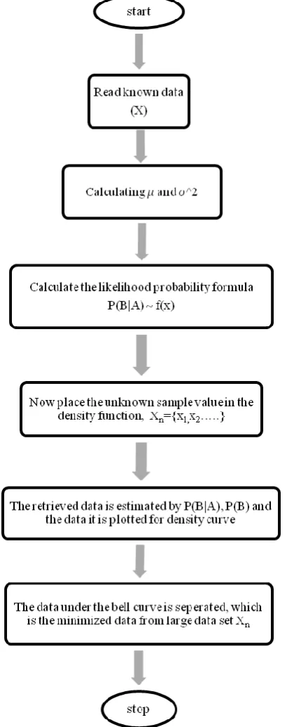
The graph shows the magnitude of voltage at various data points on a single phase. This procedure is repeated for remaining phases to get the required sample data sets.Then mean and covariance values are calculated by using these constructed data sets.

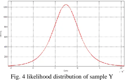
Values which are obtained after the evaluation is get substitute in the Gaussian process to get the values of X at x1…xn. The Bayesian approach discussed in earlier parts the entire data set is consider being the likelihood to estimate the posterior distribution.

Fig. 4 likelihood distribution of sample Y

Now the new observation Y as y1…..yn is made it will processed to the already existing likelihood p(Y) to estimate the posterior distribution p(X|Y). This means every time a new set of values is available, when the set Y is placed in the posterior distribution. The data that received from the distribution function (data under the bell) is separated. The valued and separated information is compared with the already existing simulated data, which are used to form a separate data sheet to train a neural network that can identify the type of fault occurred on the power system.

VIII. ARTIFICIAL NEURAL NETWORK

Fig. 5 neural network architecture

Lower back propagation [19] neural community is employed in this fault detection procedure. It's miles a feedback type machine that makes use of errors signal to modify the weights of the neural network to get the desired output this is the method calculates the gradient of loss function with respect to all weights within the network. The gradient [16] is “fed to the optimization technique which in turn uses it to update the weights, in an attempt to minimize the loss feature. A two-layer feed-forward network with sigmoid hiddenneurons and linear output neurons can healthy multi-dimensional mapping [17] troubles arbitrarily well, given constant statistics and enough neurons in its hidden layer. The network will be skilled with backpropagation algorithm, until there is not sufficient reminiscence, in which case scaled conjugate gradient backpropagation may be used. The simulated community includes input layer, hidden layer, output layer. It feed with line voltage values at the side of the time axis. The network here is the use of ‘trinelm’ trining function. Trainlm is a community education feature that updates weight and bias values in keeping with levenberg-marquardt optimization. Trainlm is often the quickest backpropagation algorithm [18] within the toolbox, and is fantastically advocated as a primary-preference supervised algorithm, even though it does require more memory than different algorithms. This feature makes use of the jacobian for calculations, which assumes that overall performance is a median or sum of squared errors. And the adaptive getting to know program used by the community is gradient boosting system characteristic. To establish a reference to the statistical framework, a gradient-descent based components of boosting methods was derived. This framework also provided the essential justifications of the version hyper parameters and established the methodological base for in addition gradient boosting model improvement. The mastering system consecutively suits new fashions to offer a extra accurate estimate of the response variable. The precept idea behind this set of rules is to construct the new base-newcomers to be maximally correlated with the poor gradient of the loss feature, associated with the whole ensemble. The reduction functions carried out can be unpredictable, but to present a exceptional consequences”. If the mistake characteristic is almost identical to the squared-error loss, the development of the neural community could result in continuous error-becoming procedure. In widespread, the staying power of the errorfunction is up to the studies method, with each a wealthy type of error capabilities derived so far and with the

possibility of implementing one's personal assignment-particular loss.

Fig. 6 neural network for fault detection

The fault detection process [5] is totally depending on predetermined values and the error that “back forwarded during process of evaluation. The output of network is a single variable with respective to the three phase line voltage. The result of the system is equivalent to respective inputs that are measured from the power lines”.

IX. EXECUTION OF SIMULATION MODEL

The model is consists of basic transmission system stages that is generation, transmission and demand side. The source side is taken as constant voltage station that delivers 230kv rms line voltage. “The 3-segment source offers a balanced 3-section voltage supply with internal r-l impedance. The three voltage sources are linked in y with a impartial connection that now not grounded. The source inner resistance and inductance can specify by using converting the source inductive short-circuit stage and x/r ratio.The source internal resistance is 0.8929 ohms (Ω).The source internal inductance is 16.58e-3 henry (H)”.

The transmission lines shown here are characterize with the pi section parameters and complete line is parted into two where the fault get created in between two pi section lines. The specifications each pi section of the transmission line is shown below as.

Positive-sequence resistances (Ohms/km) [ r1 ]=0.01273 Zero-sequence resistances (Ohms/km) [ r0 ]=0.3864 Positive- sequence inductances (H/km) [ l1]=0.9337e-3 Zero-sequence inductances (H/km) [ l0]=4.1264e-3 Positive- sequence capacitances (F/km) [ c1]=12.74e-9 Zero-sequence capacitances (F/km) [ c0]=7.751e-9 Line size (km)=100

International Journal of Innovative Technology and Exploring Engineering (IJITEE) ISSN: 2278-3075,Volume-8 Issue-6, April 2019 When fault occurred on the line, voltage waveform gets

distorted and gives harmonic content. The bus at the receiving end measure the three phase voltage and fed the values to the neural network which was trained. The ANN classifies the fault type by evaluating the given input to it.

Type of fault Trained input Output of neural network

AB 1 1.6

AG 2 2.6

BC 3 2.8

BG 4 3.9

AC 5 5.1

CG 6 5.9

ABC 7 6.8

NO_FAULT 0 0.5

Table. Output of ANN for different types of faults

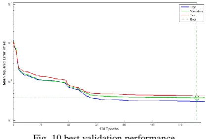
The neural network trained here on the input which is optimized by the Bayesian process. The data that received at the beginning was separated by highest probability rate which categorized into faulty and non-faulty readings. This sequential process is one time process to display the above shown output.

Fig. 10 best validation performance

X.CONCLUSION

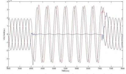
In thispaper “The Bayesian optimization method was used to optimize the sample data and converges to required result with minuscule amount of error due to repeated data points and tiny error in calculation of weights of neural network. The objective of fault identification by comparing the slight variation values ofthe detail signal in different phases. The Gaussian process algorithm for the Bayes theory allows us to estimate the true region and that give access to explore the behaviour of power system faults by using different types of data set. The evaluated posterior distribution divulges probabilistic density of each individual data point in the unknown data set that goes under Gaussian distribution. So the algorithm depends on the pre-recorded data and post-recording data sets to confine the fault type. The following figure explains the difference between the normal data set and optimized data” set.

Fig. 11 output of neural network compared with input when Bayesian optimization applied to unknown dataset

Fig. 12 output of neural network compared with input when Bayesian optimization not applied to unknown dataset

Gaussian process can fit a wide range of smooth normal distribution surface while being “computationally traceable even for moderate to large number of predictors. The posteriors are used to select the next query point as well. This algorithm is simple and flexible in terms of conditioning and inference. The main weakness of the process is it need to process a lot of unknown data samples to generate a small collection of data set that which under the curve of normal distribution”.

REFERENCES

1. TuranGonen,”Third Edition, Electrical Power Transmission System Engineering, Analysis and Design”, pp.537-630. May 2014.

2. Pooja.P, Preethi.K.R, Prof. Chetan H R, Prof.Nandish B M, “Three Phase Transmission Line Fault Analysis using Matlab Simulink”. International Journal of Scientific Development and Research.May 2016 IJSDR. 3. J.Lewis Blackburn, ThamousJ.Domin,” Third Edition, Protective Relaying

Principles and Application”, pp.105-159. December 2006.

4. Avagaddi Prasad, J. Belwin Edward, K. Ravi. “A Review on Fault Classification Methodologies in Power Transmission Systems: Part-II”.

Journal of Electrical Systems and Information Technology.October 2016doi: 10.1016/j.jesit.2016.10.003.

5. Ashish Maheshwari, Dr. Sanjeev Sharma, “Classification of Fault Identification Techniques in Power System Transmission Lines”. Journal of Emerging Technologies and Innovative Research. January 2018. 6. Alok Mukherjee, PalashKundu, ArabindaDas,”Identification and

Classification of Power System Faults using Ratio Analysis of Principal Component Distances”.Telkomnika Indonesian Journal of Electrical Engineering, November 2014 doi: 10.11591/telkomnika.v12i11.6496. 7. Eric Brochu, Vlad M. Cora and Nando de Freitas,”A Tutorial on Bayesian

8. Javier Molinero Velasco,” A Bayesian Network approach to diagnosing the root cause of failure from trouble tickets”. December 2012, doi: 10.5430/air.v1n2p75.

9. Sham Kakade and Greg Shakhnarovich,”Nearest Neighbor Rules”, Large Scale Learning, Lecture-5. July 2009.

10.Anna pernestal,” A Bayesian Approach to Fault Isolation with Application to Diesel Engine Diagnosis”.Stockholm, Sweden 2007.

11.Daniel Berrar,Bayes’ Theorem and Naïve BayesClassifier. Tokyo Institute of Technology (2018). doi:10.1016/B978-0-12-809633-8.20473-1. 12.Wei Chu, ZoubinGhahramani,”Gaussian Processes for Ordinal

Regression”. Journal of Machine Learning Research. May 2005. 13.Michael A. Osborne, Roman Garnett, and Stephen J. Roberts,” Gaussian

Processes For Global Optimization”. University of Oxford, January 2009. 14.Luc Devroye, Laszlo Gyorfi, Gabor Lugosi,” A Probabilistic Theory of

Pattern Recognition”. Springer (2009).

15.Phillip Boyle,” Gaussian Processes ForRegressionAndOptimisation”.Victoria University of Wellington (2007).

16.H. Balaga, D. N. Vishwakarma,”Artificial Neural Network Based Backup Differential Protection of Generator-Transformer Unit”.International Journal of Electronics and Electrical Engineering. December 2015. doi: 10.12720/ijeee.3.6.482-487.

17.Avagaddi Prasad, J. Belwin Edward, C. Shashank Roy, G. Divyansh and AbhayKumar,”Classification of Faults in Power Transmission Lines using Fuzzy-Logic Technique”.Indian Journal of Science and Technology.November 2015. doi: 10.17485/ijst/2015/v8i30/77065. 18.KarthikeyanKasinathan,” Power System Fault Detection And

Classification By Wavelet Transformer And Adaptive Resonance Theory Neural Networks”.University of Kentucky (2006).

19.Priyanka Pawar, Prof.NileshMohota,”Hand Gesture Recognition Using Back Prorogation Algorithm Based on Neural Network”. International Journal on Recent and Innovation Trends in Computing and Communication.July 2015. ISSN: 2321-8169.

AUTHORS PROFILE

Narni Vijaya Kumar born in vijayawada1985. He persud his bachelor degree (B.Tech) in Electrical and Electronics at Sasi Institute of Technology and Engineering in 2007. He got his masters degree (M.Tech) in JNTU-hyderabad specialization in electrical power engineering in 2009.at present he was working as assistant professor at godavari institute of engineering and technology rajahmundry.