Cloud Technologies for Bioinformatics Applications
Xiaohong Qiu
1, Jaliya Ekanayake
1,2, Scott Beason
1, Thilina Gunarathne
1,2,
Geoffrey Fox
1,21
Pervasive Technology Institute,
2School of Informatics and Computing,
Indiana University
Bloomington IN, U.S.A.
{ xqiu, jekanaya, smbeason, tgunarat, [email protected]}
Roger Barga
3, Dennis Gannon
33
Microsoft Research
Microsoft Corporation
Redmond WA, U.S.A
{Barga, [email protected]}
ABSTRACT
Executing large number of independent tasks or tasks that perform minimal inter-task communication in parallel is a common requirement in many domains. In this paper, we present our experience in applying two new Microsoft technologies Dryad and Azure to three bioinformatics applications. We also compare with traditional MPI and Apache Hadoop MapReduce implementation in one example. The applications are an EST (Expressed Sequence Tag) sequence assembly program, PhyloD statistical package to identify HLA-associated viral evolution, and a pairwise Alu gene alignment application. We give detailed performance discussion on a 768 core Windows HPC Server cluster and an Azure cloud. All the applications start with a “doubly data parallel step” involving independent data chosen from two similar (EST, Alu) or two different databases (PhyloD). There are different structures for final stages in each application.
Categories and Subject Descriptors
C.4 PERFORMANCE OF SYSTEMS; D.1.3 Concurrent Programming; E.5 FILES; J.3 LIFE AND MEDICAL SCIENCES
General Terms
Algorithms, Performance.Keywords
Cloud, bioinformatics, Multicore, Dryad, Hadoop, MPI
1.
INTRODUCTION
There is increasing interest in approaches to data analysis in scientific computing as essentially every field is seeing an exponential increase in the size of the data deluge. The data sizes imply that parallelism is essential to process the information in a timely fashion. This is generating justified interest in new runtimes and programming models that unlike traditional parallel models such as MPI, directly address the data-specific issues.
Experience has shown that at least the initial (and often most time consuming) parts of data analysis are naturally data parallel and the processing can be made independent with perhaps some collective (reduction) operation. This structure has motivated the important MapReduce paradigm and many follow-on extensions. Here we examine four technologies (Dryad [1], Azure [2] Hadoop [8] and MPI) on three different bioinformatics application (PhyloD [3], EST [4, 5] and Alu clustering [6, 7]). Dryad is an implementation of extended MapReduce from Microsoft and Azure is Microsoft’s cloud technology. All our computations were performed on Windows Servers with the Dryad and MPI work using a 768 core cluster Tempest consisting of 32 nodes each of 24-cores. Each node has 48GB of memory and four Intel six core Xenon E7450 2.4 Ghz chips. All the applications are (as is often so in Biology) “doubly data parallel” (or “all pairs” [24]) as the basic computational unit is replicated over all pairs of data items from the same (EST, Alu) or different sources (PhyloD). In the EST example, each parallel task executes the CAP3 program on an input data file independently of others and there is no “reduction” or “aggregation” necessary at the end of the computation, where as in the Alu case, a global aggregation is necessary at the end of the independent computations to produce the resulting dissimilarity matrix that is fed into traditional high performance MPI. PhyloD has a similar initial stage which is followed by an aggregation step. In this paper we evaluate the different technologies showing they give similar performance in spite of the different programming models.
In section 2, we describe the three applications EST, PhyloD and Alu sequencing while the technologies are discussed in section 3 (without details of the well known Hadoop system). Section 4 presents some performance results. Conclusions are given in section 6 after a discussion of related work in section 5.
2.
APPLICATIONS
2.1
EST and its software CAP3
An EST (Expressed Sequence Tag) corresponds to messenger RNAs (mRNAs) transcribed from the genes residing on chromosomes. Each individual EST sequence represents a fragment of mRNA, and the EST assembly aims to re-construct full-length mRNA sequences for each expressed gene. Because ESTs correspond to the gene regions of a genome, EST sequencing has become a standard practice for gene discovery, Permission to make digital or hard copies of all or part of this work
for personal or classroom use is granted without fee provided that copies are not made or distributed for profit or commercial advantage and that copies bear this notice and the full citation on the first page. To copy otherwise, or republish, to post on servers or to redistribute to lists, requires prior specific permission and/or a fee.
especially for the genomes of many organisms that may be too complex for whole-genome sequencing. EST is addressed by the software CAP3 which is a DNA sequence assembly program developed by Huang and Madan [4]. that performs several major assembly steps: these steps include computation of overlaps, construction of contigs, construction of multiple sequence alignments, and generation of consensus sequences to a given set of gene sequences. The program reads a collection of gene sequences from an input file (FASTA file format) and writes its output to several output files, as well as the standard output.
We have implemented a parallel version of CAP3 using Hadoop [8], CGL-MapReduce [12], and Dryad but we only report on a new Dryad study here.
[image:2.612.78.267.244.402.2]2.2
PhyloD
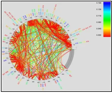
Figure 1. Pictorial representation of PhyloD output.
PhyloD is a statistical package to identify HLA-associated viral evolution from the given sample data. It is available today as a web application [13] and as downloadable source code [11]. Running PhyloD jobs is a compute intensive process. PhyloD-Cloud is an effort to leverage Windows Azure as a computing platform and create a scalable web-based application to process PhyloD jobs. Users should be able to submit reasonably large jobs using this web application with minimal manual involvement.
The package is used to derive associations between HLA alleles and HIV codons and between codons themselves. The uniqueness of PhyloD comes from the fact that it takes into consideration the phylogenic evolution of the codons for producing its results. The package takes as input the phylogenic tree information of the codons, the information about presence or absence of HLA alleles and the information about presence or absence of HIV codons. It fits its inputs to a generative model and computes a ‘p-value’, a measure of the association between HLA alleles and the HIV codons. For a set of such computed p-values, the package may also compute a ‘q-value’ per p-value which is an indicative measure of the significance of the result. Figure 1 presents the output of one such run. Arcs indicate association between codons, colors indicate q-values of the most significant association between the two attributes.
At a high level, a run of PhyloD does the following: (i) compute a cross product of input files to produce all allele-codon pairs, (ii) For each allele-codon pair, compute p value, and (iii) using the p values from the previous step, compute the q value for each allele-codon pair. The computation of p value for an allele-allele-codon pair
can be done independently of other p value computations and each such computation can use the same input files. This gives PhyloD its “data-parallel” characteristics namely, (i) ability to partition input data into smaller logical parts and (ii) workers performing same computation on data partitions without much inter-process communication.
2.3
Alu Sequence Classification
The Alu clustering problem [7] is one of the most challenging problems for sequencing clustering because Alus represent the largest repeat families in human genome. There are about 1 million copies of Alu sequences in human genome, in which most insertions can be found in other primates and only a small fraction (~ 7000) are human-specific. This indicates that the classification of Alu repeats can be deduced solely from the 1 million human Alu elements. Notable, Alu clustering can be viewed as a classical case study for the capacity of computational infrastructures because it is not only of great intrinsic biological interests, but also a problem of a scale that will remain as the upper limit of many other clustering problem in bioinformatics for the next few years, e.g. the automated protein family classification for a few millions of proteins predicted from large metagenomics projects. In our work here we examine Alu samples of 35339 and 50,000 sequences.
3.
TECHNOLOGIES EXPLORED
3.1
Dryad
Dryad is a distributed execution engine for coarse grain data parallel applications. It combines the MapReduce programming style with dataflow graphs to solve the computation tasks. Dryad considers computation tasks as directed acyclic graph (DAG) where the vertices represent computation tasks and with the edges acting as communication channels over which the data flow from one vertex to another. The data is stored in (or partitioned to) local disks via the Windows shared directories and meta-data files and Dryad schedules the execution of vertices depending on the data locality. (Note: The academic release of Dryad only exposes the DryadLINQ API for programmers [9, 10]. Therefore, all our implementations are written using DryadLINQ although it uses Dryad as the underlying runtime). Dryad also stores the output of vertices in local disks, and the other vertices which depend on these results, access them via the shared directories. This enables Dryad to re-execute failed vertices, a step which improves the fault tolerance in the programming model.
3.2
Azure
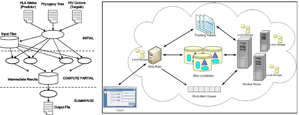
Figure 2. Architecture of a typical Azure application
[image:2.612.319.549.541.647.2]Amazon S3 etc., Azure offers a collection of discrete scalable components known as “roles” along with a set of storage and communication components. The architecture of a typical Azure
application is shown infigure 2.
The web role and the worker role represent the processing components of an Azure application. The web role is a web application accessible via HTTP or HTTPs endpoints and is hosted in an environment that supports subset of ASP.NET and Windows Communication Foundation (WCF) technologies. Worker role is the main processing entity in the Azure platform which can be used to execute functions written in managed code, scripts, or standalone executables on data products. Both web role instances and worker role instances can access the storage services.
Azure Queues are First in, First Out (not guaranteed) persistent communication channels which can be used to develop complex communication patterns among a set of corporation worker roles and web roles. A set of tasks/jobs can be organized as a collection of messages in an Azure queue and a set of workers can be deployed to remove a message (a task/job) from the queue and execute it. Azure provides three types of storage services Blob, Queue, and Table. The blob represents a persistence storage services comprising of collection of blocks. The user can store data (or partitioned data) in blobs and access them from web and worker role instances. Azure Tables provides structured storage for maintaining service state. The Azure blobs and Queues have close similarities to the Amazon Elastic Block storage and Simple Queue Service.
3.3
Old Fashioned Parallel Computing
One can implement many of the functionalities of Dryad or Hadoop using classic parallel computing including threading and MPI. MPI in particular supports “Reduce” in MapReduce parlance through its collective operations. The “Map” operation in MPI, is just the concurrent execution of MPI processes in between communication and synchronization operations. There are some important differences such as MPI being oriented towards memory to memory operations whereas Hadoop and Dryad are file oriented. This difference makes these new technologies far more robust and flexible. On the other the file orientation implies that there is much greater overhead in the new technologies. This is a not a problem for initial stages of data analysis where file I/O is separated by a long processing phase. However as discussed in [6], this feature means that one cannot execute efficiently on MapReduce, traditional MPI programs that iteratively switch between “map” and “communication” activities. We have shown that an extension CGL-MapReduce can support both classic MPI and MapReduce operations and we will comment further in section 4.3 on this. CGL-MapReduce has a larger overhead than good MPI implementations but this overhead does decrease to zero as one runs larger and larger problems.
Simple thread-based parallelism can also support “almost pleasingly parallel” applications but we showed that under Windows, threading was significantly slower than MPI for Alu sequencing. This we traced down to excessive context switching in the threaded case. Thus in this paper we only look at MPI running 24 processes per node on the Tempest cluster. Note that when we look at more traditional MPI applications with substantial communication between processes, one will reach different conclusions as use of hybrid threaded on node-MPI between node strategies, does reduce overhead [6].
4.
PERFORMANCE ANALYSIS
[image:3.612.320.554.72.251.2]4.1
EST and CAP3
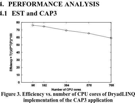
Figure 3. Efficiency vs. number of CPU cores of DryadLINQ implementation of the CAP3 application
We implemented a DryadLINQ application that performs CAP3 sequence assembly program in parallel. As discussed in section 2.1 CAP3 is a standalone executable that processes a single file containing DNA sequences. To implement a parallel application for CAP3 using DryadLINQ we adopt the following approach: (i) the input files are partitioned among the nodes of the cluster so that each node of the cluster stores roughly the same number of input files; (ii) a “data-partition” (A text file for this application) is created in each node containing the names of the input files available in that node; (iii) a DryadLINQ “partitioned-file” (a meta-data file understood by DryadLINQ) is created to point to the individual data-partitions located in the nodes of the cluster.
Then we used the “Select” operation available in DryadLINQ to apply a function (developed by us) on each of these input sequence files. The function calls the CAP3 executable passing the input file name and other necessary program parameters as command line arguments. The function also captures the standard output of the CAP3 program and saves it to a file. Then it moves all the output files generated by CAP3 to a predefined location.
This application resembles a common parallelization requirement, where an executable, a script, or a function in a special framework such as Matlab or R, needs to be applied on a collection of data items. We can develop DryadLINQ applications similar to the above for all these use cases.
We measured the efficiency of the DryadLINQ implementation of the CAP3 application using a data set of 2304 input files by varying the number of nodes used for processing. The result of
this benchmark is shown in figure 3.The collection of input files
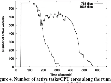
maps/reducers (in MapReduce) or vertices (in Dryad) is handled based on the availability of data and the computation power and not by the priorities. To verify the above observation we measured the utilization of vertices during two runs of the CAP3 program. In our first run we used 768 input files so that Dryad schedules 768 vertices on 768 CPU cores, while in the second Dryad schedules 1536 vertices on 768 CPU cores. The result of this benchmark is shown in figure 4.
Figure 4. Number of active tasks/CPU cores along the running times of two runs of CAP3.
The first graph in figure 4 corresponding to 768 files indicates that although DryadLINQ starts all the 768 vertices at the same time they finish at different times with long running tasks taking roughly 40% of the overall time. The second graph (1536 files) shows that the above effect has caused lower utilization of vertices when Dryad schedules 1536 vertices to 768 CPU cores. This is due to the way Dryad schedule tasks to compute nodes and we have discussed this behavior extensively in [10]. We would not expect the same behavior (for graph 2) in other MapReduce implementations such as Hadoop, however, still the non-uniformity of the processing time of parallel tasks and the simple scheduling adopted by the MapReduce runtimes may not produce optimal scheduling of tasks.
4.2
PhyloD
The parallel solution of PhyloD can be visualized as consisting of the following three different phases as shown in Figure 2 (left).
Initial – During this phase, the input files are collected from the user and copied to a shared storage available to all workers. Then a sufficient number of workers are instantiated, each with the information of the data partition it has to work on. To reduce the parallel overhead, a worker can process multiple allele-codon
pairs. ComputePartial – Each worker processes its allotted
partition and produces intermediate results. These results are again copied to a shared storage.
Summarize – During this phase, each of the intermediate results
produced during the ComputePartial phase are aggregated and the
final output is produced.
We developed an Azure application for the PhyloD application by utilizing Azure Web Role, Worker Role, Blob Container, Work Item Queue and Tracking tables described in sec. 3.2 generally and their use in PhyloD is shown in Figure 2 (Right). The web role is a simple ASP.NET application that allows clients to upload input files and provide other job parameters. A blob container is created per job which hosts the shared data between web and
worker roles. The uploaded input files are copied to this container
and an Initial work item is enqueued in the shared queue by the
web role. Worker roles continuously poll the work item queue for
new messages. A message encapsulates one of {Initial,
ComputePartial, Summarize} work items. The evaluation of these work items is delegated to their respective processors. The processors return a Boolean result for the evaluation. The calling worker then removes the message from the queue or leaves it there based on the results of the evaluation.
While processing an Initial work item, a worker role first tries to
locate the entry for this task in the JobSteps table. If the job step is not found then it means that the web role enqueued the work item and then encountered some error before creating the job step entry in the table storage. No further action is taken in this case and the job is marked ‘Aborted’. If the job step entry is found and its status is ‘Completed’ we just remove this message from the queue. A ‘Completed’ status indicates that a worker has already
processed this work item successfully but could not delete the
message from the queue due to, for example, network errors or message timeout. After these checks are satisfied, the worker updates the status of parent job to ‘In Progress’. It then enqueues
multiple ComputePartial work items in the queue and also creates
corresponding job steps in the JobSteps table. Each
ComputePartial work item has the partition information. The
worker then enqueues a Summarize work item and creates its
corresponding job step. Finally, it updates the status of Initial job
step to ‘Completed’ and removes the Initial work item from the
queue. ComputePartial work items are processed by multiple
worker roles simultaneously. Each worker processes its allotted partition of the input data and copies the intermediate results to the blob container. PhyloD engine works exclusively on files. So, a pre-processing task of copying the original input files to worker
role’s local storage is required for each ComputePartial work
item. The worker follows similar checks for the status as in the
Initial processing. Finally, the Summarize work item is processed. Intermediate results are aggregated to produce the final output which is again copied back to the blob container. The results can be downloaded via the web role. During the complete process, status information is updated in azure tables for tracking purposes.
We are currently developing a DryadLINQ application for the PhyloD data analysis where the set of tasks are directly assigned to a collection of vertices where each of them process some number of tasks and give intermediate results. Unlike in Azure
[image:5.612.59.561.114.307.2]implementation, in Dryad case, the intermediate results can directly be transferred to a vertex for aggregation to produce the final output.
[image:5.612.70.278.328.644.2]Figure 6. Efficiency vs. number of worker roles in PhyloD prototype run on Azure March CTP
Figure 7. Number of active Azure workers during a run of PhyloD application.
4.3
Alu Sequence Classification
4.3.1
Complete Problem with MPI and MapReduce
This application uses two highly parallel traditional MPI applications MDS (Multi-Dimensional Scaling) and Pairwise (PW) Clustering algorithms described in Fox, Bae et al. [6]. The latter identifies sequence families as relatively isolated as seen for example in figure 8. MDS allows visualization by mapping the high dimension sequence data to three dimensions for visualization.
Figure 8. Alu: Display of Alu families from MDS calculation from 35339 sequences using SW-G distances. The younger
families AluYa, AluYb show tight clusters
MDS has a very formulation as it finds the best set of 3D vectors x(i) such that a weighted least squares sum of the difference between the sequence dissimilarity D(i,j) and the Euclidean distance |x(i) - x(j)| is minimized. This has a computational
complexity of O(N2) to find 3N unknowns for N sequences. It can
[image:5.612.318.560.438.603.2]Maximization and use of traditional excellent χ2 minimization methods. The latter are used here.
The PWClustering algorithm is an efficient MPI parallelization of a robust EM (Expectation Maximization) method using annealing (deterministic not Monte Carlo) originally developed by Ken Rose, Fox [14, 15] and others [16]. This improves over clustering methods like Kmeans which are sensitive to false minima. The original clustering work was based in a vector space (like Kmeans) where a cluster is defined by a vector as its center. However in a major advance 10 years ago [16], it was shown how one could use a vector free approach and operate with just the distances D(i,j). This method is clearly most natural for problems like Alu sequences where currently global sequence alignment (over all N sequences) is problematic but D(i,j) can be precisely
calculated. PWClustering also has a time complexity of O(N2) and
in practice we find all three steps (Calculate D(i,j), MDS and PWClustering) take comparable times (a few hours for 50,000 sequences) although searching for a lot of clusters and refining the MDS can increase their execution time significantly. We have presented performance results for MDS and PWClustering elsewhere [6, 17] and for large datasets the efficiencies are high (showing sometimes super linear speed up). For a node architecture reason, the initial distance calculation phase reported below has efficiencies of around 40-50% as the Smith Waterman computations are memory bandwidth limited. The more complex MDS and PWClustering algorithms show more computation per data access and high efficiency.
4.3.2
Structure of all pair distance processing
The Alu sequencing problem shows a well known factor of 2
issue present in many O(N2) parallel algorithms such as those in
direct simulations of astrophysical stems. We initially calculate in parallel the Distance D(i,j) between points (sequences) i and j. This is done in parallel over all processor nodes selecting criteria i < j (or j > i for upper triangular case) to avoid calculating both D(i,j) and the identical D(j,i). This can require substantial file transfer as it is unlikely that nodes requiring D(i,j) in a later step will find that it was calculated on nodes where it is needed.
The MDS and PWClustering algorithms described in section 4.3.1, require a particular parallel decomposition where each of N processes (MPI processes, threads) has 1/N of sequences and for this subset {i} of sequences stores in memory D({i},j) for all sequences j and the subset {i} of sequences for which this node is responsible. This implies that we need D(i,j) and D(j,i) (which are equal) stored in different processors/disks. This is a well known collective operation in MPI called either gather or scatter but we did not use this in current work. Rather we designed our initial calculation of D(i,j) so that efficiently we only calculated the independent set but the data was stored so that the later MPI jobs could efficiently access the data needed. We chose the simplest approach where the initial phase produced a single file holding the full set of D(i,j) stored by rows – all j for each successive value of i. We commented in introduction that the initial phase is “doubly data parallel” over i and j whereas the MPI algorithms have the straightforward data parallelism over just a single sequence index i; there is further the typical iterative communication-compute phases in both MDS and PWClustering that implies one needs extensions of MapReduce (such as CGL-MapReduce) if you wish to execute the whole problem in a single programming paradigm. In both MDS and PWClustering, the only MPI primitives needed are MPI Broadcast, AllReduce, and Barrier so it will be quite elegantly implemented in CGL-MapReduce.
4.3.3
Smith Waterman Dissimilarities
We identified samples of the human and Chimpanzee Alu gene sequences using Repeatmasker [18] with Repbase Update [19]. We have been gradually increasing the size of our projects with the current largest samples having 35339 and 50000 sequences and these require a modest cluster such as Tempest (768 cores) for processing in a reasonable time (a few hours as shown in section 4.3.6). Note from the discussion in section 4.3.2, we are aiming at supporting problems with a million sequences -- quite practical today on TeraGrid and equivalent facilities given basic analysis
steps scale like O(N2). We used open source version NAligner
[20] of the Smith Waterman – Gotoh algorithm SW-G [21, 22] modified to ensure low start up effects by each thread/processing large numbers (above a few hundred) at a time. Memory bandwidth needed was reduced by storing data items in as few bytes as possible. In the following two sections, we just discuss the initial phase of calculating distances D(i,j) for each pair of sequences so we can efficiently use either MapReduce and MPI.
4.3.4
Dryad Implementation
We developed a DryadLINQ application to perform the calculation of pairwise SW-G distances for a given set of genes by adopting a coarse grain task decomposition approach which requires minimum inter-process communicational requirements to ameliorate the higher communication and synchronization costs of the parallel runtime. To clarify our algorithm, let’s consider an example where N gene sequences produces a pairwise distance matrix of size NxN. We decompose the computation task by considering the resultant matrix and groups the overall computation into a block matrix of size DxD where D is a multiple (>2) of the available computation nodes. Due to the symmetry of the distances D(i,j) and D(j,i) we only calculate the distances in the blocks of the upper triangle of the block matrix as shown in figure 9 (left). Diagonal blocks are specially handled and calculated as full sub blocks. As number of diagonal blocks D and total number D(D+1)/2, there is no significant compute overhead added. The blocks in the upper triangle are partitioned (assigned) to the available compute nodes and an “Apply” operation is used to execute a function to calculate (N/D)x(N/D) distances in each block, where d is defined as N/D. After computing the distances in each block, the function calculates the transpose matrix of the result matrix which corresponds to a block in the lower triangle, and writes both these matrices into two output files in the local file system. The names of these files and their block numbers are communicated back to the main program. The main program sort the files based on their block number s and perform another “Apply” operation to combine the files corresponding to a row of blocks in a single large row block as shown in the figure 9 (right).
4.3.5
MPI Implementation of Distance Calculation
and MPI). We provide options for any combinations of thread vs. process vs. node but in earlier papers [6, 17], we have shown as discussed in section 3.3 that threading is much slower than MPI for this class of problem. We explored two different algorithms
termed “Space Filling” and “Block Scattered” below. In each case, we must calculate the independent distances and then build the full matrix exploiting symmetry of D(i,j).
[image:7.612.113.500.120.272.2][image:7.612.106.501.302.462.2]
Figure 9. Task decomposition (left) and the DryadLINQ vertex hierarchy (right) of the DryadLINQ implementation of SW-G pairwise distance calculation application.
Figure 10. Space Filling MPI Algorithm: Task decomposition (left) and SW-G implementation calculation (right).
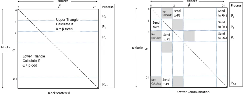
The “Space Filling” MPI algorithm is shown in figure 10, where the data decomposition strategy runs a "space filling curve through lower triangular matrix" to produce equal numbers of pairs for each parallel unit such as process or thread. It is necessary to map indexes in each pairs group back to corresponding matrix coordinates (i, j) for constructing full matrix later on. We implemented a special function "PairEnumertator" as the convertor. We tried to limit runtime memory usage for performance optimization. This is done by writing a triple of i, j, and distance value of pairwise alignment to a stream writer and the system flashes accumulated results to a local file periodically. As the final stage, individual files are merged to form a full distance matrix. Next we describe the “Block Scattered” MPI algorithm shown in figure 11. Points are divided into blocks such that each processor is responsible for all blocks in a simple decomposition illustrated in the figure 11 (Left). This also illustrates the initial computation, where to respect symmetry, we
calculate half the D(α,β) using the following criterion:
If β >= α, we only calculate D(α,β) if α+β is even while in the lower triangle, β < α, we only calculate D(α,β) if α+β is odd.
This approach can be applied to points or blocks. In our implementation, we applied to blocks of points -- of size (N/P)x(N/P) where we use P MPI processes. Note we get better load balancing than the “Space Filling” algorithm as each
processor samples all values of β. This computation step must be
followed by a communication step illustrated in Figure 11 (Right) which gives full strips in each process. The latter can be straightforwardly written out as properly ordered file(s).
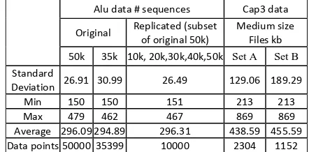
Alu data # sequences Cap3 data Original Replicated (subset of original 50k) Medium size Files kb 50k 35k 10k, 20k,30k,40k,50k Set A Set B
Standard
Deviation 26.91 30.99 26.49 129.06 189.29 Min 150 150 151 213 213 Max 479 462 467 869 869 Average 296.09294.89 296.31 438.59 455.59 Data points5000035399 10000 2304 1152
Table 1: Mean and Standard Deviation of Alu & CAP3 data
0
..
..
(0,d-1) (0,d-1)
Upper triangle
0
1
2
D-1
0 1 2 D-1
NxN matrix broken down to DxD blocks
Blocks in lower triangle are not calculated directly
0
(0,2d-1) (0,d-1)
0 ((D-1)d,Dd-1)D-1
(0,d-1)
D
(0,d-1) (d,2d-1)
D+1
(d,2d-1) (d,2d-1)
((D-1)d,Dd-1) ((D-1)d,Dd-1)
DD-1
0 1 DD-1
V V V
..
..
V V V
..
DryadLINQ vertices
File I/O DryadLINQ
vertices
Each D consecutive blocks are merged to form a set of row blocks each with NxD elementsprocess has workload of NxD elements
Blocks in upper triangle
0 1 1T 1 2T DD-1
V 2
File I/O File I/O
M =
0 1 Nx(N-1)/2
P0 P1
..
PP..
T0M/P M/P M/P
T0 T0 T0 T0 T0
I/O I/O I/O
..
Merge files File I/O MPI
Threading
Each process has workload of M/P elements
Indexing
0
2 1
N(N-1)/2
..
..
(1,0)
(2,0) (2,1)
(N-1,N-2)
Lower triangle
0
1
2
N-1
0 1 2 N-1
Space filling curve
[image:7.612.326.547.590.699.2]4.3.6
Alu SW-G Distance Calculation Performance
We present a summary of results for both Dryad and MPI computations of the Alu distance matrix in figures 12 and 13. We used several data sets and there is inhomogeneity in sequence size throughout these sets quantified in table 1. Two of 35,339 and [image:8.612.96.523.132.299.2]50,000 sequences were comprised of distinct sequences while we also prepared datasets allowing us to test scaling as a function of dataset size by taking 10,000 sequences and replicating them 2-5 times to produce 10K, 20K, 30K, 40K, 50K “homogeneous” or replicated datasets.
[image:8.612.63.280.342.518.2]Figure 11. Block Scattered MPI Algorithm: Decomposition (Left) and Scattered Communication (Right) to construct full matrix.
Figure 12. Performance of Dryad implementation of SW-G (note that the Y-axis has a logarithmic scale)
Figure 13. Comparison of Dryad and MPI on SW-G alignment on replicated and original raw data samples
In figure 12, we present Dryad results for the replicated dataset showing the dominant compute time compared to the small partition and merge phases. Further for the Block Scattered MPI approach, the final “scatter” communication takes a negligible time. Figure 13 compares the performance of Dryad and the two MPI approaches on the homogeneous (10K – 50K) and heterogeneous (35K, 50K) datasets. We present the results as the time in milliseconds per distance pair per core. This is measured total time of figure 12 multiplied by number of cores and divided by square of dataset size i.e. it is time a single core would take to calculate a single distance. Then “perfect scaling in dataset size or number of nodes” should imply a constant value for this quantity. We find that for Dryad and MPI, the replicated dataset time is roughly constant as a function of sequence number and the original 35339 and 50,000 sequence samples are just a little slower than the replicated case. Note from table 1, that there is little variation in measure of inhomogeneity between replicated and raw data. A surprising feature of our results is that the Space Filling MPI algorithm is faster than the Block Scattered approach. Dryad lies in between the two MPI implementations and is about 20% slower on the replicated and heterogeneous dataset compared to Space-Filling MPI. We are currently investigating this but given the complex final data structure, we see that it is impressive that the still preliminary Dryad implementation does very well.
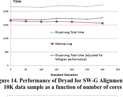
[image:8.612.56.291.546.684.2]In figure 14, we show that Dryad scales well with number of nodes in that time per distance pair per core is roughly constant on the 10K replicated SW-G data and consistent with Dryad replicated data points in figure 13. In table 1, we showed that SW-G is more homogeneous than CAP3 in that standard deviation/mean is lower. However we also got reasonable scaling in figure 3 for CAP3 which corresponds to data set A of table 1 while preliminary results for the more heterogeneous “Set B”, also shows good scaling from 192 to 576 cores. The dependence on data homogeneity is very important and needs better study and perhaps dynamic scheduling or more
D blocks 0 1 D-1 2 β α D blocks 0 D-1 Upper Triangle Calculate if
α+ βeven
Lower Triangle Calculate if
α+ βodd
Process P0 P1 P2 PP-1 Block Scattered D blocks 0 1 D-1 2 β α D blocks
0 D-1 Process
P0
P1
P2
PP-1
Send to P2
Send to PD-1 Send to PD-1 Send to PD-1 Send
to P0
Send to P1
Send to P1
1 2 Not Calculate Not Calculate Not Calculate
Scatter Communication
1 10 100 1000 10000 100000
0 10000 20000 30000 40000 50000 60000
Ti m e (s e co n d s) Sequences
Dyrad Implementation of SW-G alignment (homogenous data) Partition Time Computation Time Merge Time Total Time 0 1 2 3 4 5 6 7
0 10000 20000 30000 40000 50000 60000
Ti m e p er d is ta nc e c al cu la ti on p er c or e (m ili se co nd s) Sequeneces
Performance of Dryad vs. MPI of SW-Gotoh Alignment
sophisticated scattering of data between processes to achieve statistical load balance.
[image:9.612.70.268.195.351.2]We study the effect of inhomogeneous gene sequence lengths for SW-G pairwise distance calculation applications. These results also present comparisons of Hadoop and Dryad on identical hardware rebooted with Linux and Windows respectively. The data sets used were randomly generated with a given mean sequence length (400) with varying standard deviations following a normal distribution of the sequence lengths.
Figure 14. Performance of Dryad for SW-G Alignment on 10K data sample as a function of number of cores
Figure 15. Performance of Dryad vs. Hadoop for SW-G for inhomogeneous data as a function of standard deviation with
mean sequence length of 400
Each data set contained a set of 10000 sequences and a 100 million pairwise distance calculations to perform. Sequences of varying lengths are randomly distributed across the data set. The Dryad-adjusted results depict the raw Dryad results adjusted for the performance difference of the NAligner (C#) and JAligner (Java) base Smith-Waterman alignment programs. As we notice from the figure 15, both the Dryad implementation as well as the Hadoop implementation performed satisfactorily, without showing significant performance degradations for high standard deviation. In fact the Hadoop implementation showed minor improvements in the execution times. The acceptable performance can be attributed to the fact that the sequences with varying lengths are randomly distributed across the data set, giving a natural load balancing to the sequence blocks. The Hadoop implementations’ slight performance improvement can be attributed to the global pipeline scheduling of map tasks that Hadoop performs. In Hadoop, the administrator can specify the map task capacity of a particular worker node and then Hadoop global scheduler schedules the map tasks directly on to those placeholders when individual tasks finish in a much finer
granularity than in Dryad. This allows the Hadoop implementation to perform natural global level load balancing.
5.
RELATED WORK
There have been several papers discussing data analysis using a variety of cloud and more traditional cluster/Grid technologies with the Chicago paper [23] influential in posing the broad importance of this type of problem. The Notre Dame all pairs system [24] clearly identified the “doubly data parallel” structure seen in all of our applications. We discuss in the Alu case the linking of an initial doubly data parallel to more traditional “singly data parallel” MPI applications. BLAST is a well known doubly data parallel problem and has been discussed in several papers [25, 26]. The Swarm project [5] successfully uses traditional distributed clustering scheduling to address the EST and CAP3 problem. Note approaches like Condor have significant startup time dominating performance. For basic operations [27], we find Hadoop and Dryad get similar performance on bioinformatics, particle physics and the well known kernels. Wilde [28] has emphasized the value of scripting to control these (task parallel) problems and here DryadLINQ offers some capabilities that we exploited. We note that most previous work has used Linux based systems and technologies. Our work shows that Windows HPC server based systems can also be very effective.
6.
CONCLUSIONS
We have studied three data analysis problems with four different technologies. The applications each start with a “doubly data-parallel” (all pairs) phase that can be implemented in MapReduce, MPI or using cloud resources on demand. The flexibility of clouds and MapReduce suggest they will become the preferred approaches. We showed how one can support an application (Alu) requiring a detailed output structure to allow follow-on iterative MPI computations. The applications differed in the heterogeneity of the initial data sets but in each case good performance is observed with the new cloud technologies competitive with MPI performance. The simple structure of the data/compute flow and the minimum inter-task communicational requirements of these “pleasingly parallel” applications enabled them to be implemented using a wide variety of technologies. The support for handling large data sets, the concept of moving computation to data, and the better quality of services provided by the cloud technologies, simplify the implementation of some problems over traditional systems. We find that different programming constructs available in cloud technologies such as independent “maps” in MapReduce, “homomorphic Apply” in Dryad, and the “worker roles” in Azure are all suitable for implementing applications of the type we examine. In the Alu case, we show that Dryad and Hadoop can be programmed to prepare data for use in later parallel MPI/threaded applications used for further analysis. Our Dryad and Azure work was all performed on Windows machines and achieved very large speed ups (limited by memory bandwidth on 24 core nodes). Similar conclusions would be seen on Linux machines as long as they can support the DryadLINQ and Azure functionalities used. The current results suggest several follow up measurements including the overhead of clouds on our Hadoop and Dryad implementations as well as further comparisons of them.
7.
ACKNOWLEDGMENTS
We thank our collaborators from Biology whose help was essential. In particular Alu work is with Haixu Tang and Mina 0
1 2 3 4 5 6 7
288 336 384 432 480 528 576 624 672 720
Ti
m
e p
er
d
is
ta
nc
e c
al
cu
la
ti
on
p
er
c
or
e
(m
ill
is
ec
on
ds
)
Cores
DryadLINQ Scaling Test on SW-G Alignment
0 500 1000 1500 2000 2500
0 50 100 150 200 250 300 350
Standard Deviation
Dryad-swg Total time
Hadoop-swg
Rho from Bioinformatics at Indiana University and the EST work is with Qunfeng Dong from Center for Genomics and Bioinformatics at Indiana University. We also thank Microsoft Research for providing data used in PhyloD and Azure applications.
8.
REFERENCES
[1] M. Isard, M. Budiu, Y. Yu, A. Birrell, D. Fetterly, “Dryad: Distributed data-parallel programs from sequential building blocks,” European Conference on Computer Systems, March 2007.
[2] Microsoft Windows Azure,
http://www.microsoft.com/azure/windowsazure.mspx
[3] C. Kadie, PhyloD. Microsoft Computational Biology Tools. http://mscompbio.codeplex.com/Wiki/View.aspx?title=Phy loD
[4] X. Huang, A. Madan, “CAP3: A DNA Sequence Assembly Program,” Genome Research, vol. 9, no. 9, pp. 868-877, 1999.
[5] S. L. Pallickara, M. Pierce, Q. Dong, and C. Kong, “Enabling Large Scale Scientific Computations for Expressed Sequence Tag Sequencing over Grid and Cloud Computing Clusters”, PPAM 2009 EIGHTH
INTERNATIONAL CONFERENCE ON PARALLEL PROCESSING AND APPLIED MATHEMATICS Wroclaw, Poland, September 13-16, 2009
[6] G. Fox, S.H. Bae, J. Ekanayake, X. Qiu, H. Yuan Parallel Data Mining from Multicore to Cloudy Grids Proceedings of HPC 2008 High Performance Computing and Grids workshop Cetraro Italy July 3 2008
http://grids.ucs.indiana.edu/ptliupages/publications/Cetraro WriteupJan09_v12.pdf
[7] M.A. Batzer, P.L. Deininger, 2002. "Alu Repeats And Human Genomic Diversity." Nature Reviews Genetics 3, no. 5: 370-379. 2002
[8] Apache Hadoop,
[9] Y.Yu, M. Isard, D. Fetterly, M. Budiu, Ú. Erlingsson, P. Gunda, J. Currey, “DryadLINQ: A System for General-Purpose Distributed Data-Parallel Computing Using a High-Level Language,” Symposium on Operating System Design and Implementation (OSDI), CA, December 8-10, 2008.
[10] J. Ekanayake, A. S. Balkir, T. Gunarathne, G. Fox, C. Poulain, N. Araujo, R. Barga. "DryadLINQ for Scientific Analyses", Technical report, Submitted to eScience 2009
[11] Source Code. Microsoft Computational Biology Tools.
[12] J. Ekanayake, S. Pallickara, “MapReduce for Data Intensive Scientific Analysis,” Fourth IEEE International Conference on eScience, 2008, pp.277-284.
[13] T. Bhattacharya, M. Daniels, D. Heckerman, B. Foley, N. Frahm, C. Kadie, J. Carlson, K. Yusim, B. McMahon, B. Gaschen, S. Mallal, J. I. Mullins, D. C. Nickle, J. Herbeck, C. Rousseau, G. H. Lear. PhyloD . Microsoft
Computational Biology Web Tools.
[14] K. Rose, “Deterministic Annealing for Clustering, Compression, Classification, Regression, and
RelatedOptimization Problems”, Proceedings of the IEEE, vol. 80, pp. 2210-2239, November 1998.
[15] Kenneth Rose, Eitan Gurewitz, and Geoffrey C. Fox “Statistical mechanics and phase transitions in clustering” Phys. Rev. Lett. 65, 945 - 948 (1990)
[16] T Hofmann, JM Buhmann “Pairwise data clustering by deterministic annealing”, IEEE Transactions on Pattern Analysis and Machine Intelligence 19, pp1-13 1997
[17] Geoffrey Fox, Xiaohong Qiu, Scott Beason, Jong Youl Choi, Mina Rho, Haixu Tang, Neil Devadasan, Gilbert Liu “Biomedical Case Studies in Data Intensive Computing” Keynote talk at The 1st International Conference on Cloud Computing (CloudCom 2009) at Beijing Jiaotong University, China December 1-4, 2009
[18] A. F. A. Smit, R. Hubley, P. Green, 2004. Repeatmasker. http://www.repeatmasker.org
[19] J. Jurka, 2000. Repbase Update: a database and an electronic journal of repetitive elements. Trends Genet. 9:418-420 (2000).
[20] Source Code. Smith Waterman Software. http://jaligner.sourceforge.net/naligner/.
[21] O. Gotoh, An improved algorithm for matching biological sequences. Journal of Molecular Biology 162:705-708 1982.
[22] T.F. Smith, M.S.Waterman,. Identification of common molecular subsequences. Journal of Molecular Biology 147:195-197, 1981
[23] I. Raicu, I.T. Foster, Y. Zhao, Many-Task Computing for Grids and Supercomputers,: Workshop on Many-Task Computing on Grids and Supercomputers MTAGS 2008. 17 Nov. 2008 IEEE pages 1-11
[24] C. Moretti, H. Bui, K. Hollingsworth, B. Rich, P. Flynn, D. Thain, "All-Pairs: An Abstraction for Data Intensive Computing on Campus Grids," IEEE Transactions on Parallel and Distributed Systems, 13 Mar. 2009, DOI 10.1109/TPDS.2009.49
[25] M. C. Schatz “CloudBurst: highly sensitive read mapping with MapReduce”, Bioinformatics 2009 25(11):1363-1369; doi:10.1093/bioinformatics/btp236
[26] K. Keahey, R. Figueiredo, J. Fortes, T. Freeman, M. Tsugawa, “Science clouds: Early experiences in Cloud computing for scientific applications”. In Cloud Computing and Applications 2008 (CCA08), 2008.
[27] J. Ekanayake, X. Qiu, T. Gunarathne, S. Beason, G. Fox “High Performance Parallel Computing with Clouds and Cloud Technologies”, Technical Report August 25 2009