This is a repository copy of
A Gaussian Process Convolution Particle Filter for Multiple
Extended Objects Tracking with Non-Regular Shapes
.
White Rose Research Online URL for this paper:
http://eprints.whiterose.ac.uk/131615/
Version: Accepted Version
Proceedings Paper:
Aftab, W., De Freitas, A., Arvaneh, M. et al. (1 more author) (2018) A Gaussian Process
Convolution Particle Filter for Multiple Extended Objects Tracking with Non-Regular
Shapes. In: 2018 21st International Conference on Information Fusion (FUSION) (FUSION
2018). 21st International Conference on Information Fusion, 10-13 Jul 2018, Cambridge,
UK. IEEE . ISBN 978-0-9964527-6-2
10.23919/ICIF.2018.8455501
[email protected] https://eprints.whiterose.ac.uk/
Reuse
Items deposited in White Rose Research Online are protected by copyright, with all rights reserved unless indicated otherwise. They may be downloaded and/or printed for private study, or other acts as permitted by national copyright laws. The publisher or other rights holders may allow further reproduction and re-use of the full text version. This is indicated by the licence information on the White Rose Research Online record for the item.
Takedown
If you consider content in White Rose Research Online to be in breach of UK law, please notify us by
A Gaussian Process Convolution Particle Filter for
Multiple Extended Objects Tracking with
Non-Regular Shapes
Waqas Aftab
The University of Sheffield Sheffield, UK [email protected]
Allan De Freitas
University of Pretoria Pretoria, South Africa [email protected]
Mahnaz Arvaneh
The University of Sheffield Sheffield, UK [email protected]
Lyudmila Mihaylova
The University of Sheffield Sheffield, UK
Abstract—Extended object tracking has become an integral part of various autonomous systems in diverse fields. Although it has been extensively studied over the past decade, many complex challenges remain in the context of extended object tracking. In this paper, a new method for tracking multiple irregularly shaped extended objects using surface measurements is proposed. The Gaussian Process Convolution Particle Filter proposed in [1], designed to track a single extended/group object, is enhanced for tracking multiple extended objects. A convolution kernel is proposed to estimate the multi-object likelihood. A target birth/death model based on the proposed method is also introduced for automatic initiation and deletion of the objects. The proposed approach is validated on real-world LiDAR data which shows that the method is efficient in tracking multiple irregularly shaped extended objects in challenging scenarios involving occlusion, dense clutter and low object detection.
I. INTRODUCTION
Recently, extended object tracking (EOT) has become a fundamental process in various autonomous systems. These systems belong to a wide spectrum of fields such as navigat-ing autonomous cars through traffic [2], autonomous human and surrounding objects tracking based on Microsoft Kinect sensors [3], tracking of hazardous clouds [4] and many more. EOT requires estimation of the kinematics and the shape of an object of interest from a sequence of noisy sensor measurements. The kinematic states include the position of the centre of the object and its higher order time derivatives. The states related to the shape of the object are commonly the extent of the object from the centre.
Object tracking is not a new area of research and dates back to the times of the second world war. Traditionally, object tracking has been referred to as multiple target tracking (MTT) [5]. MTT deals only with the estimation of the ob-ject kinematics. It is also referred as point obob-jects tracking (POT) [6] and [7]. The state estimation of the kinematics states in the EOT is done using the methods similar to those proposed in the traditional MTT literature [8], [9]. The focus of the EOT research has been on the shape estimation methods and the measurement models. The different methods proposed over time have been extensively covered in the two overview papers [6], [7]. Typically, the object kinematics are modelled in the global frame while the object shape is modelled in the object centered frame.
Similarly to the POT, the tracking of a single extended object is comparatively simpler to the problem of tracking
multiple extended objects. A single EOT problem provides a solution to the challenges of unknown object kinematics, shape and shape dynamics, measurement error and uncertainty of the measurements origin using Bayesian inference methods. The object kinematics models are inherited from the literature of the POT. Various shape models have been proposed for the single EOT. These include techniques which model the object shape as a basic geometric shape, e.g. tracking of a cyclist using a stick model [7], a car using a rectangular model [10], a ship using an ellipsoidal model [11] etc. Although these methods have been proved to be simple and efficient on real-world data, the shapes of these and other extended objects are different to the basic geometric shapes. The tracking accuracy increases as the precision of the shape estimation increases [7]. Some advanced shape estimation methods have also been proposed for tracking the object as an irregularly shaped (star-convex) object. These include the random hypersurface model (RHM) [12], Gaussian Process (GP) based models [13], [1] and mixture of sub-objects [14].
The measurement models include the measurement source and clutter model and the sensor measurement error model. The complexity of the methods increases when the measure-ments are received from the surface of the object. In such scenarios, the RHM and the GP model of [13] are sensitive to the statistical properties of the measurements coming from the object, which might be unknown in real-world scenarios. The analytical expression of the measurement likelihood is also not available due to the non-linearity of the problem. The Gaussian Process Convolution Particle Filter (GPCPF) [1] does not require any prior knowledge of measurement statistics and an analytical expression of the likelihood function. Moreover, unlike the method proposed in [13], this method can track a single object moving in clutter.
performance for classification of multiple objects. However, advanced clustering and inference techniques are required when the objects come close or cross each other. In such sce-narios, the most likely sets of measurement clusters are used for inference. A stochastic optimisation based method [16] has been demonstrated to track closely moving objects by proposing an efficient method to determine the most likely sets. In this paper, a GPCPF based method is proposed for tracking of multiple extended objects with non-regular shapes.
A. Contributions
The contributions of this work are as follows; (i) A new Gaussian process convolution particle filter (GPCPF) based approach for tracking multiple extended objects having non-regular shapes is proposed. A GPCPF for tracking a single extended object is proposed in [1]. (ii) A new convolutional kernel is proposed to track different complex shaped objects using surface measurements without any prior knowledge of the measurement statistics. The typical complex-shaped multiple extended objects tracking methods require prior in-formation of the object size or the statistical properties of the measurements [17], [18]. (iii) A new object birth/death model based on the likelihood estimation using convolu-tion kernel is proposed. This framework treats the object detection, false-alarm rejection, object existence and death in a probabilistic framework without the requirement of an explicit likelihood function. (iv) The performance validation of the proposed method on real data from extended objects is presented in the results section.
The structure of the paper is as follows. The system dynamical model is presented in Section II, the theoretical background of GP and GPCPF is described in Section III, the proposed multiple EOT GPCPF is given in Section IV, the performance validation and results are given in Section V followed by conclusions in Section VI.
II. SYSTEMMODEL
A. System Dynamics Model
The dynamics of the centre of the object (COO) are assumed independent of those of the object shape. The discrete time COO state update equation is given below:
ck = (INg,k⊗F
c
)ck−1+w
c
k−1, (1) where ck =
h
c1kT , c2kT
,· · · , cNg,k
k
TiT represents the multiple objects COO state vector, In represents an n
-dimensional identity matrix, (·)T represents the transpose
operation, Ng,k represents the number of extended objects at
time k, Fc represents the single object COO state transition matrix,wc
k−1∼ N 0,INg,k⊗Q
c
represents the COO model process noise, Qc represents the process noise covariance of the COO of a single object and(.)k represents that the vector
/ matrix corresponds to time k. The extent states dynamics is modelled as a random walk [1] and is described by the following equation:
sk = (INg,k⊗IB)sk−1+w
s
k−1, (2) where sk =
h
s1kT , s2kT
,· · · , sNg,k
k
TiT represents the
multiple objects extent state vector, wsk−1 ∼ N 0,INg,k⊗ Qs
represents the extent dynamics model noise, Qs
repre-sents the process noise covariance of a single object extent dynamics. The Qs can be modelled based on the prior knowledge of the objects being tracked, e.g. if the objects are axis-symmetric then an axis-symmetric covariance kernel can be used to determine this matrix. If there is no prior knowledge of the object shape, then it can be modelled as given below [1]:
Qs=σe2IB, (3)
whereσ2
e represents the variance of the change in extent per
sample time. B. State Vector
The multiple objects state vectorXk is given below:
Xk=
h
(x1k)T (x2
k)T · · · (x Ng,k
k )T
iT
, (4)
xik=
(cik)T (si k)T
T
, (5)
where xik represents the ith object state, ci
k represents the
states related to the centre andsik denotes the states related to the shape (extent) of the ith object. The extent states consist
of the radial extent of the object at B different angles from the COO. The COO and the extent states are given below:
cik = xi
k x˙ik yik y˙ik
T
, (6)
sik =
ri,k1 rki,2 · · · rki,BT. (7) where(xi
k, yik)and( ˙xik,y˙ik)represent the position and velocity
of theithobject’s COO.ri,j
k represents the radial value of the ith object at the jth angle of the input vectorθb
. The input angle vector is given below:
θb=
θ1 θ2 · · · θBT
, θl= (l−1)2π
B. (8) C. Shape Model and the GP
The shape of the object is assumed to be star-convex1 and
is modelled using a Gaussian Process (GP) model as proposed in [13]. The extent is modelled as a function of the angle from the COO. This mapping function for anithobject is given by
the following equation:
ri=fi(θ), (9) whererirepresents the true radial values andfirepresents the
true mapping function of theithobject. The function maps the
continuous domainθ to the rangesr. As the object can have any arbitrary shape hence fi is a non-linear function and a
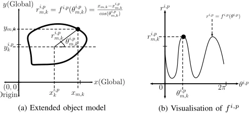
GP is used to estimate this mapping function. This is further realised in Figs 1a and 1b. A Von Mises covariance kernel [1] is used:
kvm(θi, θj′) =σ
2
feσ
2
acos(θi−θ′j), (10)
where σ2
f, σ2a control the magnitude and the length-scale of
the kernel, respectively. D. Measurement Model
The sensor reports measurements in Cartesian coordinates and the measurement noise is assumed to be independent and identically distributed Gaussian. The measurement equation is given below:
zk =H(Xk) +vk, vk ∼ N(0,Σk), (11)
Σk =diag(R1,k,R2,k,· · · ,RNk,k), (12) 1A polygon is called star-convex, if all line segments from its center to the
x(Global)
y(Global)
xik,p
yi,pk
b
xm,k
ym,k
θi,pm,k
(0,0)
ri,pm,k=fi,p(θ i,p m,k) =
xm,k−xi,pm,k
cos(θi,p m,k)
Origin
ri,pm,k
(a) Extended object model
b
0 2π
rim,k,p
θm,ki,p
θi,p
ri,p
ri,p=fi,p(θi,p)
(b) Visualisation offi,p
Fig. 1: (a) Fig. 1a shows an ith extended object (thick solid
line) in the global Cartesian frame. The sensor measurements and the COO kinematics are modelled in the global frame. The extent states are modelled in the polar frame local to each object. The ith object’s local frame has origin located
at (xi,pk , yi,pk ). The radial extent r of the object is modelled as a function f of the angle θ in the local frame given by r = f(θ). The coordinates of the mth measurement are
shown in the global and theithobjects local frame. The
non-linear relation between the two frames is also presented for this measurement. (b) Fig. 1b visualises the non-linear radial functionf of Fig. 1a. The origin corresponds to the centre of theithobject. Themthmeasurement is shown for comparison.
where zk = [zT1,k,z2T,k,· · ·,zTNk,k]
T denotes the
measure-ment vector,Nk represents the total number of measurements,
H(·) represents the non-linear measurement function, vk is
the measurement noise vector, Σk is the measurement noise
covariance matrix, zm,k = [xm,k, ym,k]T represents the mth
measurement, (xm,k, ym,k) are the Cartesian coordinates of
the mth measurement, R
m,k = diag(σx2m, σ
2
ym) is the
cor-responding measurement noise covariance matrix, σ2xm, σ
2
ym
represent the sensor noise variances in thexandydimensions, respectively and diag(·)represents a diagonal matrix.
III. THEORETICALBACKGROUND
A. Gaussian Process
A GP is a stochastic process for mapping non-linear func-tions from an input to an output space. The GP is defined by a mean and a covariance kernel. The parameters of the mean and the covariance kernel are called hyperparameters. These hyperparameters are learned using training data. A trained and learned GP can be used to determine the output at input locations other than those present in the training data. An elaborate account of the GP and its applications can be found in [19].
Let the input and output spaces be represented by the random vectors θ andr, respectively. A GP, mathematically represented as GP(µ(θ),C(θ,θ′)), is described by a non-linear function f given below:
r=f(θ), (13)
C(θ,θ′) =
k(θ1, θ1′) k(θ1, θ′2) ... k(θ1, θ′N) k(θ2, θ1′) k(θ2, θ′2) ... k(θ2, θ′N)
..
. ... ... ... k(θN, θ′1) k(θN, θ2′) ... k(θN, θN′ )
, (14)
where the mean of the GP is generally modelled as a constant,
[image:4.612.52.299.63.175.2]C(θ,θ′)is the covariance matrix of the GP and k(·,·)is the
TABLE I: GP-CPF Recursion
1 fork≤2,θB= 0 : 360/B: 360Initialise statex0
2 fork= 3findx˜n0 =N(x0, σ2x0),w n 0 =
1 N
3 fork >3Re-sample : Residual Re-sampling as in [20]. 4 fork≥3
4a State Sample: forn= 1,2, ...N ˜
xn
k =Fx˜ n k−1+wk
4b Measurement Simulation : Simulate measurements using the measurement model
4c Measurement Gating : A measurement is considered gated if it lies within the region of the measurement sample 4d Weight Update : forn= 1,2, ...N find
wn k =
QL
l=1K z
h(zk,l)×wnk−1
4e Normalise Weight : forn= 1,2, ...N determine
wn k =
wkn
PN n=1wnk 4f Estimation :pn
k(xk|z1:K) =PNn=1w n kx˜
n k
corresponding covariance kernel. Let θ′ ∈RN and r′
repre-sent the training data input and output vectors, respectively. The GP regression equation for an unknown input vector θ⋆
is given below:
p(r⋆|θ⋆) =N(Cθ⋆θ′(Cθ′θ′+σ2IN)
−1r′,Cθ⋆θ⋆
−Cθ⋆θ′(Cθ′θ′+σ2IN)−1Cθ′θ⋆), (15)
where r⋆ represents the output vector, (·)−1 represents the matrix inverse and σ2 is measurement noise variance.
B. Gaussian Process Convolution Particle Filter
The GPCPF [1] tracks an irregularly shaped extended object moving through clutter using noisy sensor measurements orig-inating from the surface of an extended object. The filter has two major components namely the GP model for the object shape and the CPF for the posterior density estimation. The GPCPF recursion is summarised in Table I.
IV. MULTIPLEGROUPOBJECTSTRACKING USING
GAUSSIANPROCESSCONVOLUTIONPARTICLEFILTER
[image:4.612.323.550.64.252.2]are then used to update the posterior density estimation using the CPF measurement kernel.
A. The Convolution Particle Filter Kernel
The CPF kernel is used for the multi-modal density es-timation. The CPF in a state space setting for the multiple objects tracking relies on two kernels. The first kernel KX
hX
is defined for the predictive distribution in the state space of state vectorX. The second kernel is defined for the likelihood estimation in the measurement spaceKz
hz of the measurement
vector z. The hX and hz represent the predictive and the
likelihood kernel bandwidths, respectively. As proposed in [1], the state vector Xk maps to multiple independent regions in
the measurement space and is equivalent to the functional-ity of the kernel KX
hX. Hence, K
X
hX is not required to be
defined explicitly. The likelihood kernel Kz
hz is defined for
measurements originating from the objects as well as clutter. This kernel has the form:
Kz
hz(z
m− ˜
Zi,pk ) =
(
UZi,p(z), zm∈ Zi,p
UV(z), zm∈ Z/ i,p
, (16)
where zm represents the mth measurement, Z˜i,p
k represents
the measurement sample of thepthparticle and theithobject,
UR represents a uniform distribution supported by the region
R, V represents the sensor coverage and Zi,p represents the ithregion in the measurement space of thepth particle. Each
particle creates Ng,k regions in the measurement space. The
uniform kernels described in (16) are given below:
UZi,p(z) =
1
Area(Zi,p), UV(z) =
1
Area(V), (17)
whereArea(·)returns the area of the region within brackets. B. State Sampling
The state sample of apthparticle at timekis given below:
˜
Xpk=h(x˜1k,p)T (
˜
x2k,p)T · · ·(
˜ xNg,k,p
k )T
iT
, (18)
˜ xi,pk =
(c˜i,pk )T (s˜i,p k )T
T
, (19)
where X˜pk represents the multiple objects state sample,x˜i,pk
represents the ith object state andc˜i,p k ands˜
i,p
k represent the ithobject COO and the extent states sample of thepthparticle.
The COO and the extent states samples are determined using equations (1) and (2), respectively.
C. Measurement Sampling
The measurement sample is given below:
˜
Zi,pk =h(z˜i,p1,k)T (z˜i,p
2,k)T · · · (z˜ i,p B,k)T
iT
, (20)
where z˜i,pb,k represents the measurement sample of the bth
extent state and is determined as follows:
˜
zi,pb,k = [˜xi,pk ,y˜i,pk ]T + [cosθb,sinθb]T ⊙
˜
si,pb,k+vb,k, (21)
vb,k ∼ N
0, diag(σ2x, σy2) ,
where(˜xi,pk ,y˜i,pk )represent the positional samples of theci,pk ,
˜
si,pb,krepresents thebthextent state sample ofsi,p
k ,⊙represents
element-wise product, vb,k represents the sensor noise and σ2
x, σ2y represent the sensor noise variances, respectively. The
measurement sample Z˜i,pk is a collection of points in the measurement space. These points are used to train the GP of theith object and thepthparticle. The GP regression (15)
is then used to define a region in the measurement space for theithobject and thepthparticle denoted asZi,p .
D. Likelihood Calculation / Weight Update
Consider Nk measurements are received at time k from
the sensor in Cartesian coordinates. To perform the likelihood calculation and the weight update, the measurements are first gated with the particle measurement samples. This gating is done in two steps. First, the measurements are gated based on their locations and subsequently, the measurement clustering information is included to improve the gating process.
As soon as the measurements are received, the measure-ment vector zk is clustered using DBSCAN [15]. For each
measurementmthe polar coordinates are determined as given below:
θi,pm,k=tan−1 ym,k−y˜i,pk xm,k−x˜i,pk
!
, (22)
ri,pm,k=
q
(xm,k−x˜i,pk )2+ (ym,k−y˜i,pk )2, (23)
where(θm,ki,p , ri,pm,k)represents the polar coordinates of themth
measurement in the local frame of the ithobject and the pth
particle. The GP is used to predict the range of theithextended
object of thepth particle at an angleθi,p
m,k as given below:
˜
ri,pm,k=Cθi,p m,kθbC
−1
θbθbs˜
i,p
k , (24)
The measurement is considered belonging to theithextended
object of thepthparticle ifri,p m,k≤˜r
i,p
m,k. The cluster identifier
vectorzc of all the gated measurements is formed. The gated
measurements are declared not-gated with the ith extended
object of the pth particle if the cluster identifier is different
from the mode ofzc or more than 15%of the measurements
with same cluster identifier are not gated. The particle weights update equation is as follows:
wki,p=wi,pk−1
Nk
Y
m=1 Khzz(z
m−Z˜i,p
k ), (25)
where wki,p represents the weight of the ith object and the pth particle. The measurements gated with one object are not
considered for updating the other objects. E. Estimation
The conditional multi-object state density can be written as:
p(Xk|Z1:k) =
p(Xk,Z1:k)
R
p(Xk,Z1:k)dXk
, (26)
where Z1:k represents all the measurements from time-step
1 to k. Along the lines of adaptive CPF modelled in [21], the kinematic and extent states are sampled separately. The estimate equations are given below:
pPk(Xk|Z1:k) = Ng,k
X
i=1
pPk(xik|Z1:k), (27)
pP
k(xik|Z1:k) =
PP
p=1w
i,p k x˜
i,p k K
z
hz(Z1:k−Z˜
p i,k)
PP
p=1K
z
hz(Z1:k−Z˜
p i,k)
, (28)
and the kernel is represented as:
Kz
hz(Z1:k−Z˜
p i,k) =
k
Y
j=1 Kz
hz(zj−Z˜
p
TABLE II: Existence processes
Process eg,k eg,k−1
Pre-birth 0 0
Birth 1 0
Existing 1 1
Death 0 1
False alarm 2 0
where P is the number of particles. The ith object state
estimate is given below
ˆ xik=
PP
p=1w
i,p k x
i,p k
PP
p=1w
i,p k
. (30)
F. Object Existence / Birth / Death Model
The objects enter, pass-through and leave the area of inter-est. The sensors can also report clutter. These are represented by different processes which are a modification of the method proposed in [22]. The entry is modelled by a pre-birth and birth process, the pass-through is modelled by an existence process while exiting is modelled by a disappearance/death process. The sensor clutter is modelled as a false alarm process. Each extended object state is augmented by an existence variable eg,k ∈ {0,1,2} which specifies the existence state of thegth
extended object at time k. The relation between the different processes and the existence variable is shown in Table II. The existence variable is assigned a value based on the object likelihood λg,k and is given below:
λg,k=
PP
p=1w
p k
QM
m=1K
z
hz(z
m−z˜g,p k )
PP
p=1w
p k
. (31)
Two thresholds are defined to detect the object process. These are the birth threshold Tb and the death threshold Td. The
thresholds are related to the existence variable as given below:
eg,k=
1 λg,k ≥Tb, eg,k−1= 0
0 λg,k < Tb, eg,k−1= 0
0 λg,k ≤Td, eg,k−1= 1
1 λg,k > Td, eg,k−1= 1
2 λg,k ≤Td, eg,k−1= 0
(32)
At any given time, the pre-birth, birth and the existing objects are part of the extended object state vectorXk. The death and
false-alarm objects are removed from this state vector at the end of the processing step. As a result, the size of this state vector changes, which is also depicted by the time-dependence of Ng,k.
The objects can appear from a region called birth region e.g it can be a door to the building entrance in a crowd tracking in a building problem. There areNb number of birth
regions in the area of interest. Each birth region is defined by a centre (xb, yb), which specifies the location of the centre
of the birth objects, an initial velocity ( ˙xb,y˙b)and a circular
region of radius rb, which specifies the initial shape of the
object. The values of these parameters can be tuned according to the application.
G. Object Merging / Splitting / Spawning
The object merging occurs by design through the gating pro-cess. The splitting/spawning can be included through a modifi-cation of the birth process. All the un-associated measurements in a particular scan are classified using DBSCAN clustering
method. All the clusters are considered as birth regions for the next scan. The mean and the variance of the measurements position are used to define the centre and the size of the birth region. As a result, the object splitting/spawning is achieved.
V. PERFORMANCEVALIDATION
A sample of publicly available real-world data is considered for the performance validation [23]. This is a recorded data of the sensors installed on a car for real-world computer vision benchmarking. The benchmarking problems are related to an autonomous vehicle project. Multiple sensors data, installed on an observer vehicle, is available for various scenarios. The sensors include two gray-scale cameras, two colour cameras and one laser scanner. The data of the laser scanner (HDL-64E LiDAR) sensor is considered for the performance evaluation of the proposed approach. The ground truth data is not available and is constructed manually using the image data from one of the colour cameras. The ground truth of the states is calculated only for those time samples when the complete object is visible in the image data.
The 3D LiDAR data is reported in the body-fixed frame of the observer vehicle. The data is synchronised with the images obtained from the cameras. A 3D to 2D transformation matrix is used to project the data on the 2D image frame. The EOT is done in the image frame and compared with the ground truth data, which is also available in the image frame.
The given data sample consists of static and moving ex-tended objects. The moving objects are considered as objects of interest for the performance validation. Hence, the static extended objects are treated as clutter. Four moving objects (cars) cross in front of the observer vehicle during a total of66
time samples. These are available in the scene at different time instants which are explained next. The first object in samples k= 1−8, the second ink= 1−22, the third ink= 18−43
and the fourth in k = 35−60. The time samples when the objects are completely visible are as follows. The first object in samplesk = 1−3, the second object in k= 3−20, the third ink= 23−39and the fourth ink= 39−55.
The different challenges in the data are a large number of the LiDAR data i.e. on average 0.1 million measurements are received per time sample, dense (static) clutter, occlusion and one of the objects is not perfectly detected by the sensor i.e. it is a stealthy object. This stealthy object poses an additional challenge of tracking similar extended objects having different measurement statistics.
as given below:
ˆ
Ea k =
1
NM C NM C
X
i=1
(ai
k−ˆaik)2, (33)
Rµk = 1
NM C NM C
X
i=1
Area(Ti k∩Eik) Area(Ti
j)
, (34)
Pkµ = 1
NM C NM C
X
i=1
Area(Ti k∩Eik) Area(Ei
k)
, (35)
where Eˆa
k represents the RMSE of the evaluation parameter a at time k, ai
k represents the true and ˆaij represents the
estimated value, Rµk andPkµ represent the mean shape recall and precision at time k, Ti
k represents the true shape, Eki
represents the estimated shape, ∩ represents the intersection of two star-convex polygons and Area(p)represents the area of the polygon p.
A. System Dynamics
The COO dynamics are modelled using a nearly constant velocity (NCV) motion model as given below:
Fc=diag(F′,F′), F′=
1 ∆T
0 1
, (36)
Qc=diag(σ2vxQ ′
, σ2vyQ ′
), Q′ =
" ∆T3
3
∆T2
2 ∆T2
2 ∆T #
, (37)
where F′ and Q′ represent the state transition matrix and the process noise covariance matrix in one dimension, respec-tively,∆Trepresents the sampling time,σ2
vx andσ
2
vy represent
the variances of the COO velocities. The extent process noise covariance is modelled using a periodic covariance kernel [19] and is given below:
Qs=Cperθbθb, k
per θ (θ, θ
′
) =σf2e−
2sin2 θ−θ′
2
l2
θ , (38)
where Cperθbθb represents a GP covariance matrix calculated
using a periodic covariance kernel kperθ (θ, θ′)
and (14), σ2
f
represents the magnitude and l2
θ represents the lengthscale
hyperparameter. B. Birth/Death Model
The objective is to track the moving objects of interest i.e. pedestrians, cyclists, vehicles etc. The birth/death model is enhanced based on the problem at hand. In order to detect and track only the moving objects, two speed thresholds are introduced in the birth/death model. These are the low speed threshold Vl and high speed threshold Vh. The objects of
interest move with speeds higher than Vland lower than Vh.
C. Measurement Clustering
The LiDAR data is in 3D. The measurements coming from the ground and from very high objects (which cannot be considered moving objects on the roads) are filtered based on the height information. The filtered data is clustered based on the depth value using 1D DBSCAN clustering. The measure-ments are then projected to the 2D image frame. The projected measurements are clustered using 2D DBSCAN clustering.
D. Parameters
The filter parameters are given as follows. The total number of time samples areK= 66, the sampling time is∆T = 0.1s,
the velocity standard deviations are σvx = 250p/s 2 and
σvy = 25p/s, the hyperparameters of the extent process noise
covariance kernel areσ2
f = 10and lθ= 0.2, the surveillance
volume isArea(V) = 1242p×345p. The hyperparameters of the GPCPF kernel are σ2
a = 401,σr2 = 1 and σf2 = 30. The
number of particles isN = 500, number of basis isB = 36, the birth threshold is Tb = 0.01, death threshold is 0.001,
the low speed threshold is Vl = 200p/s and the high speed
threshold is Vh = 1000p/s. The 1D DBSCAN clustering
parameters areepsilon= 1.25and the minimum number of points are 24. The 2D DBSCAN clustering parameters are epsilon= 50and the minimum number of points are80. The sensor noise variances areσ2
x=σy2= 0.0025.
E. Results
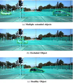
The challenging scenarios and the tracking results at three chosen time samples are shown in Fig 2. The statistical properties of the sensor measurements coming from object 3 (black car), shown in Fig. 2c, are different from those of the other three objects. The measurement density is different from the other similar objects. The proposed algorithm detects and tracks this object, which shows that the proposed method is not sensitive to the statistical properties of the sensor measurements.
The mean cardinality results are shown in Fig. 3. A delay in the object detection can be observed for all four objects. This is due to the fact that the shape is not detected in the initial time steps as the complete object is not visible. Moreover, a moving object can be determined from the data of minimum2
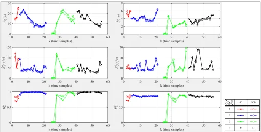
time samples. An error in the cardinality is observed between samples 20−25. It is due to the fact that the measurement statistics of the black car change considerably during these time samples. A large number of particles can be used to improve the cardinality at these time samples at the expense of computational time. The average state estimate errors are shown in Fig. 4. The positional RMSE inxis less than25p,y is less than7p,x˙ is less than110p/sandy˙ is less than30p/s. The mean shape recall is greater than0.9for most of the time steps, which shows that more than90% of the true shape has been recalled all the time. The mean shape precision is more than0.8 most of the time which shows that less than 20%of the estimated shape is false.
The program was run on MATLAB R2016b and a Win-dows 10 (64 bit) Desktop computer installed with an In-tel(R) Core(TM) i5-6500 CPU @ 3.20GHz(4 CPUs) and 8GB RAM. The computational time is 52s per time sample for N = 500particles. This is due to the large number of sensor measurements received at each time sample. The processing time is improved to 4.5s using N = 50 particles. The mean cardinality and the state estimate errors for N = 50 are also given in the Figs 3 and 4, respectively. It can be observed that all four objects are tracked and there is no false alarm. The performance of the state estimates is almost similar and the cardinality estimates are slightly degraded. The processing time can be further improved by optimizing the code and running in C++.
(a)Multiple extended objects
(b)Occluded Object
[image:8.612.316.564.53.250.2](c)Stealthy Object
Fig. 2: Challenging scenarios. The projected LiDAR data (cyan dots) is overlayed on the camera image. The ground truth object is represented by the (green) solid line and the estimated object is represented by (yellow) dotted lines. The ground truth COO is represented by (green) plus and the estimated COO is represented by (yellow) diamond. (a) Two moving extended objects (cars) are tracked whereas the static extended objects (signal post, trees etc.) are treated as clutter. (b) The moving object (white car) is occluded by two static extended objects. (c) The front half of the car is picked up by the sensor while few measurements are reported from the back half of the car. The statistical properties of the sensor measurements are also different from the other moving and static extended objects.
VI. CONCLUSIONS
The paper proposes a novel GPCPF based approach for tracking irregularly shaped multiple extended objects moving through clutter. The GPCPF along with measurement clus-tering track the extended objects as a mixture of Gaussian state samples and measurement simulations. The performance evaluation of the approach is done on real-world data. The proposed filter is able to track non-regular shaped objects in challenging scenarios like dense clutter, occlusion and low detection. In future, the GPCPF will be enhanced to the tracking scenarios involving closely moving irregularly shaped extended objects.
ACKNOWLEDGMENT
We acknowledge the support from the Pakistan Air Force (Govt. of Pakistan) and the Dept. of ACSE (University of Sheffield) for the scholarships awarded to the first author. We appreciate the support of the SETA project funded from the European Unions Horizon 2020 research and innovation programme under Grant Agreement No. 688082.
10 20 30 40 50 60
k (time samples)
00.5 1 1.5 2
True N = 50 N = 500
Fig. 3: Mean cardinality. The figure shows the true (blue thick line) and mean estimated cardinality using N = 500
(green circle line) and N = 50 (red dot line). It can be observed that although dense clutter is present, no false alarms are observed.
REFERENCES
[1] W. Aftab, A. De Freitas, M. Arvaneh, and L. Mihaylova, “A Gaussian process approach for extended object tracking with random shapes and for dealing with intractable likelihoods,” inthe Proceedings of the 22nd International Conference on Digital Signal Processing (DSP). IEEE, 2017, pp. 1–5.
[2] F. Kunz, D. Nuss, J. Wiest, H. Deusch, S. Reuter, F. Gritschneder, A. Scheel, M. St¨ubler, M. Bach, P. Hatzelmann et al., “Autonomous driving at Ulm University: A modular, robust, and sensor-independent fusion approach,” inProceedings of the IEEE Intelligent Vehicles Sym-posium (IV). IEEE, 2015, pp. 666–673.
[3] F. Faion, M. Baum, and U. D. Hanebeck, “Tracking 3D shapes in noisy point clouds with random hypersurface models,” inthe Proceedings of the 15th International Conference on Information Fusion. IEEE, 2012, pp. 2230–2235.
[4] F. Septier, A. Carmi, and S. Godsill, “Tracking of multiple contaminant clouds,” in the Proceedings of the 12th International Conference on Information Fusion. IEEE, 2009, pp. 1280–1287.
[5] B. Samuel and P. Robert, “Design and analysis of modern tracking systems,”London: Artech House, 1999.
[6] L. Mihaylova, A. Y. Carmi, F. Septier, A. Gning, S. K. Pang, and S. Godsill, “Overview of Bayesian sequential Monte Carlo methods for group and extended object tracking,”Digital Signal Processing, vol. 25, pp. 1–16, 2014.
[7] K. Granstrom, M. Baum, and S. Reuter, “Extended object tracking: Intro-duction, overview and applications,”arXiv preprint arXiv:1604.00970, 2016.
[8] S. Blackman and R. Popoli, “Design and analysis of modern tracking systems (Book),”Norwood, MA: Artech House, 1999., 1999.
[9] Y. Bar-Shalom, X. R. Li, and T. Kirubarajan,Estimation with applica-tions to tracking and navigation: theory algorithms and software. John Wiley & Sons, 2004.
[10] K. Granstr¨om, S. Reuter, D. Meissner, and A. Scheel, “A multiple model PHD approach to tracking of cars under an assumed rectangular shape,” inthe Proceedings of the 17th International Conference on Information Fusion. IEEE, 2014, pp. 1–8.
[11] K. Granstr¨om, A. Natale, P. Braca, G. Ludeno, and F. Serafino, “PHD extended target tracking using an incoherent X-band radar: Preliminary real-world experimental results,” inthe Proceedings of the 17th Inter-national Conference on Information Fusion. IEEE, 2014, pp. 1–8. [12] M. Baum and U. D. Hanebeck, “Random hypersurface models for
[image:8.612.49.302.55.343.2]0 10 20 30 40 50 60 k (time samples)
0 10 20 30
0 10 20 30 40 50 60
k (time samples) 0
2 4 6 8
0 10 20 30 40 50 60
k (time samples) 0
50 100 150
0 10 20 30 40 50 60
k (time samples) 0
10 20 30
0 10 20 30 40 50 60
k (time samples) 0
0.5 1
0 10 20 30 40 50 60
k (time samples) 0
0.5 1
50 500
N Obj
1
2
3
4
b
b
b
b
b
c
b
c
b
c
b
[image:9.612.51.561.53.312.2]c
Fig. 4:State Errors. The state estimation errors are shown for the four moving objects (obj-1 in red, obj-2 in blue, obj-3 in green and obj-4 in black) for two different number of particles that is N = 500(solid line with dots) andN = 50(solid line with circles). The positional errors are given in the top two, the velocity errors in the middle and the shape errors are given in the bottom two subplots. The errors are depicted only for those time samples when both the ground truth and the estimated states are available. The distance unit is in the frame of reference of the image that is pixels (p).
[13] N. Wahlstr¨om and E. ¨Ozkan, “Extended target tracking using Gaussian processes,”IEEE Transactions on Signal Processing, vol. 63, no. 16, pp. 4165–4178, 2015.
[14] B. Lei, C. Li, and H. Ji, “Nonlinear maneuvering non-ellipsoidal extended object tracking using random matrix,” inthe Proceedings of the 20th International Conference on Information Fusion. IEEE, 2017, pp. 1–6.
[15] M. Ester, H.-P. Kriegel, J. Sander, X. Xu et al., “A density-based algorithm for discovering clusters in large spatial databases with noise.” inKdd, vol. 96, no. 34, 1996, pp. 226–231.
[16] K. Granstr¨om, S. Renter, M. Fatemi, and L. Svensson, “Pedestrian track-ing ustrack-ing Velodyne data–Stochastic optimization for extended object tracking,” inIntelligent Vehicles Symposium (IV), 2017 IEEE. IEEE, 2017, pp. 39–46.
[17] M. Baum, B. Noack, and U. D. Hanebeck, “Mixture random hypersur-face models for tracking multiple extended objects,” inthe Proceedings of the 50th IEEE Conference on Decision and Control and European
Control Conference (CDC-ECC). IEEE, 2011, pp. 3166–3171.
[18] T. Hirscher, A. Scheel, S. Reuter, and K. Dietmayer, “Multiple extended object tracking using Gaussian processes,” inthe Proceedings of the 19th International Conference on Information Fusion (FUSION), 2016. IEEE, 2016, pp. 868–875.
[19] C. E. Rasmussen, “Gaussian processes in machine learning,” in Ad-vanced lectures on machine learning. Springer, 2004, pp. 63–71. [20] J. S. Liu and R. Chen, “Sequential Monte Carlo methods for dynamic
systems,”Journal of the American statistical association, vol. 93, no. 443, pp. 1032–1044, 1998.
[21] D. Angelova, L. Mihaylova, N. Petrov, and A. Gning, “A convolution particle filtering approach for tracking elliptical extended objects,” in
the Proceedings of the 16th International Conference on Information Fusion, 2013, pp. 1542–1549.
[22] S. K. Pang, J. Li, and S. J. Godsill, “Detection and tracking of coordinated groups,”IEEE Transactions on Aerospace and Electronic Systems, vol. 47, no. 1, pp. 472–502, 2011.
[23] A. Geiger, P. Lenz, C. Stiller, and R. Urtasun, “Vision meets robotics: The Kitti dataset,”International Journal of Robotics Research (IJRR),
2013.